Importance of the Long-Term Seasonal Component in Day-Ahead Electricity Price Forecasting Revisited: Parameter-Rich Models Estimated via the LASSO

Abstract

Recent studies suggest that decomposing a series of electricity spot prices into a trend-seasonal and a stochastic component, modeling them independently, and then combining their forecasts can yield more accurate predictions than an approach in which the same parsimonious regression or neural network-based model is calibrated to the prices themselves. Here, we show that significant accuracy gains can also be achieved in the case of parameter-rich models estimated via the least absolute shrinkage and selection operator (LASSO). Moreover, we provide insights as to the order of applying seasonal decomposition and variance stabilizing transformations before model calibration, and propose two well-performing forecast averaging schemes that are based on different approaches for modeling the long-term seasonal component.

1. Introduction

The trend-seasonal pattern of electricity spot prices, which is also known as the long-term seasonal component (LTSC), has always attracted the attention of energy analysts [1,2,3,4,5,6,7]. This is especially so when modeling the average daily prices in the medium- or the long-term. On the other hand, the short-term electricity price forecasting (EPF) literature has generally ignored it and considered models with only intra-day and intra-week periodicities, as the LTSC was believed to add unnecessary complexity. Nowotarski and Weron [8] only recently introduced the seasonal component (SC) approach and the seasonal component autoregressive (SCAR) models that decompose the electricity spot price series into a trend-seasonal and stochastic component, predict them independently, and then combine their day-ahead forecasts. The seasonal component approach works well for autoregressive (AR) [7,9] as well as non-linear autoregressive (NARX) neural network-type models [10], in the context of point and probabilistic predictions [11]. However, the studies that have been published to date may be criticized for only utilizing parsimonious structures with a relatively small number of explanatory variables or features. Additionally, these are known to underperform when compared to parameter-rich models with hundreds of regressors that are estimated via the least absolute shrinkage and selection operator (LASSO) [12,13,14,15,16]. To the best of our knowledge, only two studies have treated the LTSC in the context of LASSO-estimated models [17,18]. However, no comparisons have been made between different variants of the LTSC or with analogous models that do not utilize seasonal decomposition. An open question remains as to whether the SC approach is also beneficial in the case of parameter-rich LASSO-estimated models and to what extent.

To this end, we perform an extensive empirical study that involves:

• Six-year-long electricity price and fundamental variables time series from two distinct power markets—Nord Pool and PJM Interconnection, providing two three-year-long test periods of hourly-resolution.
• Two commonly used approaches for modeling the LTSC of electricity price series—one based on wavelet smoothing [2,3,4,5,7] and one on the Hodrick-Prescott (HP) filter [4,10,19,20].
• A parameter-rich, LASSO-estimated autoregressive model with nearly 130 regressors, after [21] called the LEAR model.
• The area hyperbolic sine (asinh) variance stabilizing transformation (VST) [22,23], which has been found to perform well when negative or close to zero electricity prices are analyzed [15,24,25,26].
• Two methods of combining point forecasts—one that selects the best combination of a pool of models (dubbed the Best Combination, BC) and one inspired by Bayesian Model Averaging (BMA) [27]. The latter weighs combinations by the inverse (of the) root mean squared error (iRMSE; similarly as in [28,29,30]), instead of the posterior probabilities that were originally proposed in [27]. We refer to it as BMA for notational convenience.
• Model validation in terms of the robust relative mean absolute errors (rMAE) and relative root mean squared errors (rRMSE) [21,31], and the Giacomini and White [32] test for significant differences in conditional predictive ability (CPA).

Because we utilize both seasonal decomposition (via the HP or the wavelet filter) and variance stabilization, a question arises regarding the order in which they should be applied. In some studies, the VST comes first [2,4,8,9,10,11], whereas in others—seasonal decomposition [18]. Not having found clear recommendations in the literature, we compare both approaches.

Our contribution is threefold. Firstly, we show that significant—as measured by the CPA test [32]—accuracy gains can be achieved by applying the seasonal component approach [8] not only to parsimonious autoregressive [7,9] or neural network [10] structures, but also to LASSO-estimated AR (LEAR) models. Provided that the performance of the latter is nearly on par with that of Deep Neural Networks (DNN) [21], this finding provides valuable insights in constructing state-of-the-art models, which do not require hyperparameter optimization and offer orders of magnitude faster execution than DNNs. Secondly, we provide insights as to the order of applying seasonal decomposition and variance stabilizing transformations before model calibration. Thirdly, we propose two well-performing forecast averaging schemes that are based on different approaches to modeling the LTSC.

The remainder of the paper is structured, as follows. In Section 2, we briefly present the datasets. Subsequently, in Section 3, we describe the methodology: the forecasting framework, the asinh transformation, seasonal decomposition, a parsimonious autoregressive model used as a benchmark, the LEAR model, and the two combination schemes. In Section 4, we measure the forecast accuracy in terms of rMAE and rRMSE, evaluate the conditional predictive ability, and comment on the computational complexity of the proposed methods. Finally, in Section 5, we wrap up the results and provide conclusions.

2. Datasets

We evaluate the considered models using datasets from two major power markets. Nord Pool is the first one, a renewable energy source dominated market in the Northern Europe, exhibiting long-term, weather-dependent fluctuations in the price levels. The second is PJM Interconnection, the world’s largest competitive wholesale electricity market covering Northeastern United States, with a coal–gas–nuclear generation mix.

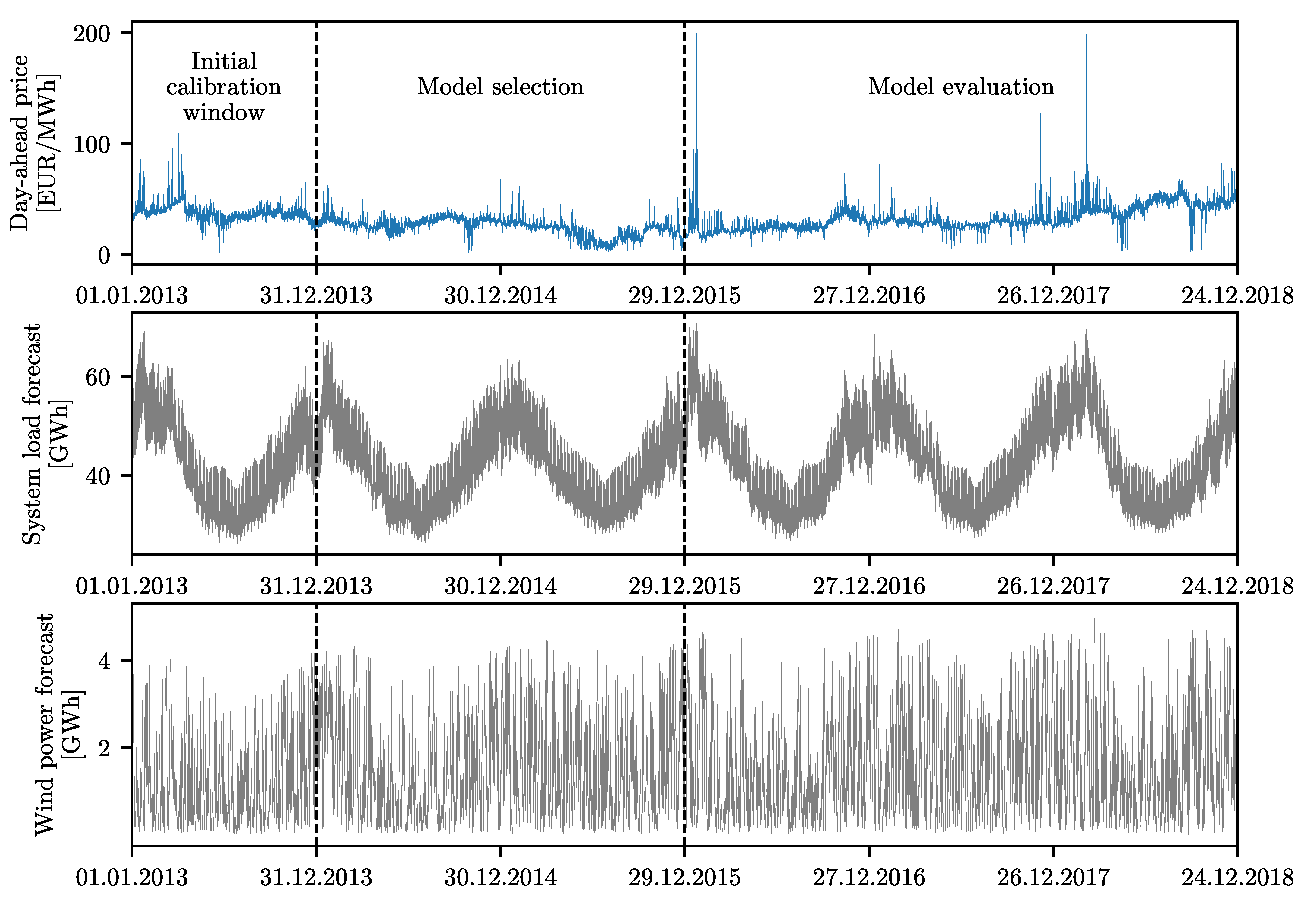
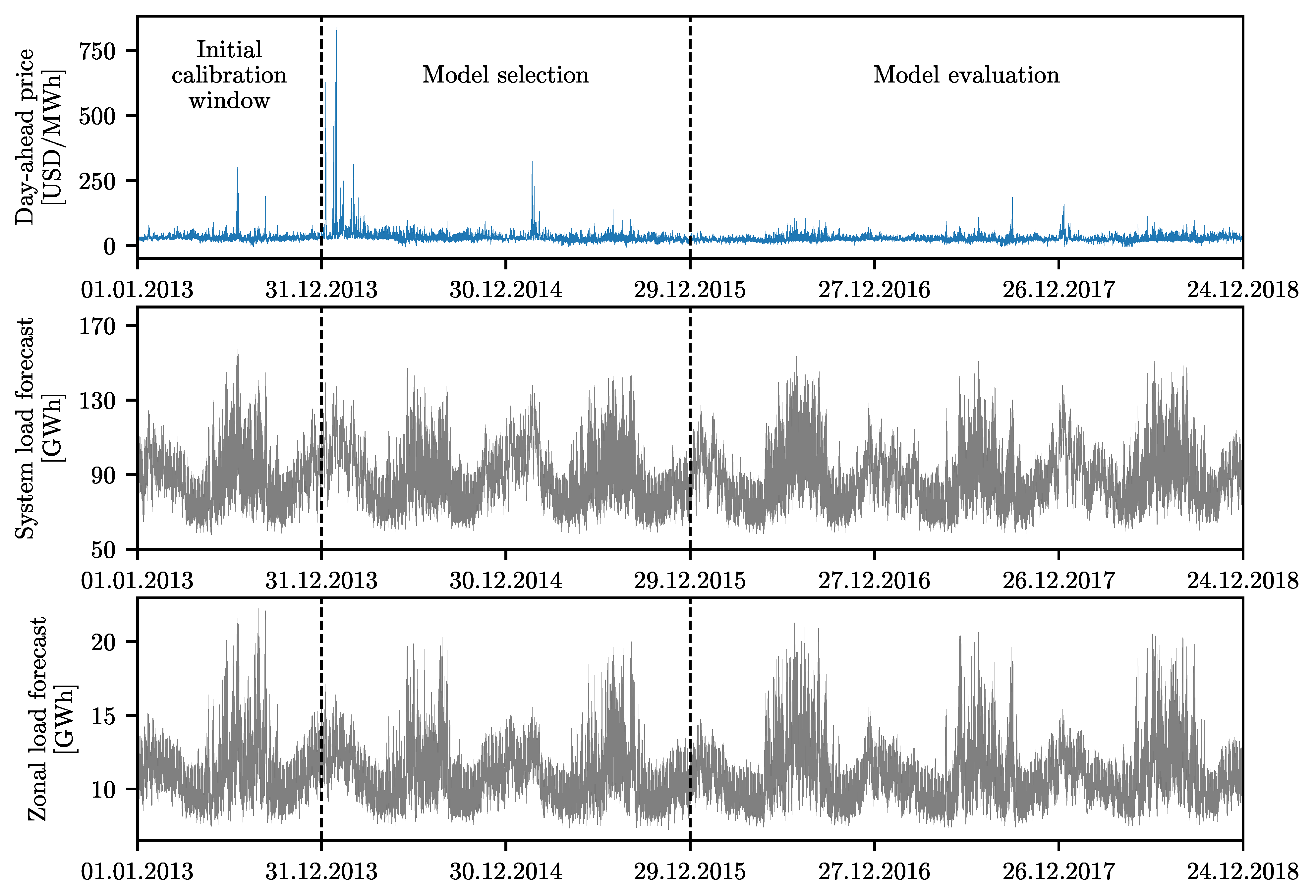
The Nord Pool (NP) dataset, as depicted in Figure 1, comprises three time series at hourly resolution: day-ahead market system prices in EUR/MWh, day-ahead system load forecasts (called consumption prognosis) for four Nordic countries (Denmark, Finland, Norway, and Sweden), and day-ahead wind power generation forecasts for Denmark. The data are freely available on the Nord Pool website www.nordpoolspot.com (accessed on 15 January 2021) The PJM dataset, as depicted in Figure 2, also comprises three time series at an hourly resolution: day-ahead market prices in the Commonwealth Edison (COMED; located in the state of Illinois) zone in USD/MWh, and two day-ahead load forecasts series—the system load and the COMED zonal load. The data are freely available on the PJM website www.pjm.com (accessed on 18 January 2021). Both of the datasets span the same six-year-long time period—from 1 January 2013 to 24 December 2018 (exactly $2184=6\times 364$ days or $\mathrm{52,416}=6\times 364\times 24$ h). It is noteworthy that, while the NP price is more volatile in the three-year-long evaluation window than in the model selection window, the PJM price exhibits the opposite behavior, see

Table 1. The summary statistics for the considered time series: the minimum value, the 1st quartile (Q1), the 2nd quartile (Q2; i.e., the median), the mean, the 3rd quartile (Q3), the maximum value, and the standard deviation. For each series, three rows report values in the initial calibration window (top), the model selection window (middle), and the model evaluation window (middle).

Time Series	Window	Min.	Q1	Q2	Mean	Q3	Max.	Std.
Nord Pool market
Day-ahead price	initial	1.38	34.30	37.45	38.13	40.90	109.55	6.94
	selection	1.14	21.38	26.27	25.34	30.61	69.94	8.01
	evaluation	2.17	25.96	30.28	33.27	39.92	199.97	11.17
System load forecast	initial	26.22	36.55	42.63	43.64	50.22	69.11	9.00
	selection	26.37	36.95	42.23	43.13	49.02	67.18	8.07
	evaluation	26.87	37.38	43.19	44.40	50.98	70.58	8.94
Wind power forecast	initial	0.03	0.43	0.92	1.24	1.87	4.20	1.00
	selection	0.02	0.55	1.25	1.53	2.38	4.45	1.14
	evaluation	0.00	0.59	1.26	1.55	2.31	5.05	1.17
PJM market
Day-ahead price	initial	$-3.24$	25.89	30.64	32.38	36.39	302.14	13.91
	selection	$-6.98$	23.80	29.42	34.13	37.56	839.30	28.80
	evaluation	$-3.62$	20.80	25.51	27.38	32.29	184.48	10.79
System load forecast	initial	57.88	80.10	89.85	91.00	100.30	157.16	15.88
	selection	58.24	79.55	89.41	91.44	102.56	149.93	16.26
	evaluation	58.35	79.42	88.39	90.72	99.98	153.31	16.29
Zonal load forecast	initial	7.46	10.00	11.37	11.57	12.67	22.24	2.26
	selection	7.25	9.80	11.17	11.33	12.52	20.30	2.08
	evaluation	7.35	9.73	11.03	11.33	12.34	21.27	2.25

with summary statistics for the analyzed time series. This will allow us to compare the models under different market conditions. Additionally, it is noteworthy that the same datasets were used in [21].

3. Methodology

We implement the multivariate modeling framework, as defined in [15], in which the predictions are separately performed for each hour. To represent our variables, we use ‘day × hour’ matrix-like structures. The day-ahead forecasts ${\widehat{p}}_{d,h|d-1}\equiv {\widehat{p}}_{d,h}$ of the electricity price $p_{d,h}$ for day d and hour h are computed on day $d-1$ using all of the information known up to that point in time. We utilize a rolling window scheme, i.e., our models are calibrated to data in a 364-day-long window and, once the 24 forecasts for all hours of the next day are made, the window is rolled forward 24 h. Subsequently, the models are calibrated again, and forecasts are computed for the next 24 h. This procedure continues until the predictions for the last day in the sample are made.

Our models involve day-ahead electricity prices and two exogenous variables, i.e., the system load and wind power forecasts for NP and system and zonal load forecasts for PJM, see Section 2 and Figure 1 and Figure 2. All three time series undergo a variance stabilizing transformation (VST; see Section 3.1, below) and seasonal decomposition (see Section 3.2, below) prior to model calibration; we consider two orders of applying these transformations—VST first, then seasonal decomposition, and vice versa. The only exceptions are the benchmark models for which seasonal decomposition is not performed. Although we use a multivariate modelling framework, both of the transformations are carried out in the calibration window for the original time series at an hourly resolution, just like in [8]. Moreover, because the forecasts of the exogenous variables are known one day in advance, in their case seasonal decomposition and variance stabilization are applied to a window that is one day longer, i.e., which covers 365 days and includes the day for which the price forecasts are made.

When it comes to forecasting, like in [8,10], the LTSC of the price time series is assumed to persist into the future (see Section 3.2, below), whereas the stochastic component is predicted based on two models with an autoregressive structure. The first one is a parsimonious ordinary least squares (OLS) estimated model, which wsa built on some prior knowledge of experts (see Section 3.3 below), whereas the second one is a parameter-rich LASSO-estimated model (see Section 3.4, below).

Finally, in Section 3.5, we propose two methods of averaging/selecting forecasts. We construct our combined predictions that are based on performance in a two-year-long model selection (or validation) window and compare them—like all the considered models—in the three-year-long evaluation (or test) window, see Figure 1 and Figure 2.

3.1. Data Transformation

A number of transformations can be used to reduce the variation in data and allow handling close to zero or negative electricity prices. Here, following [15,18,22], we resort to the area hyperbolic sine (asinh), which is a simple, but well performing, variance stabilizing transformation (VST). Before applying it, we normalize each series $x_{d,h}$, i.e., prices or load/wind forecasts, using its median ${\mathrm{Med}}_{\tau }$ and median absolute deviation ${\mathrm{MAD}}_{\tau }$ in the calibration window $\tau$:

$$y_{d,h}=\frac{1}{z_{0.75}}\frac{x_{d,h}-{\mathrm{Med}}_{\tau }}{{\mathrm{MAD}}_{\tau }},$$

(1)

where $z_{0.75}$ is the 75th percentile of the standard normal distribution and it ensures asymptotically normal consistency to the standard deviation. Such a normalization is more robust to outliers than the one based on the mean and standard deviation and, thus, it is preferred for spiky data [23]. Having normalized our variables, we apply the VST:

$$z_{d,h}=\mathrm{asinh}\left(y_{d,h}\right)=log\left(y_{d,h}+\sqrt{y_{d,h}^2+1}\right).$$

(2)

The forecasts are obtained for models that were calibrated to the VST-transformed series, after applying the inverse transformation:

$$x_{d,h}=\frac{{\mathrm{MAD}}_{\tau }}{z_{0.75}}\sinh \left(z_{d,h}\right)+{\mathrm{Med}}_{\tau },$$

(3)

where $\sinh$ is the hyperbolic sine. Because the latter is a nonlinear function, given random variable X, $\mathbb{E}\sinh \left(X\right)$ does not have to equal $\sinh \left(\mathbb{E}X\right)$. Hence, from the probabilistic point of view, Equation (3) is not the correct inverse transformation. Although this problem is generally ignored in the literature, Narajewski and Ziel [33] argue that using the correct transformation yields better forecasts. On the other hand, when the forecasts are averaged, the differences between the two approaches seem to vanish [34]. Because we eventually consider forecast combinations, to keep it simple, we use Equation (3) as the inverse transformation.

3.2. Seasonal Decomposition

Seasonal decomposition is a term that generally refers to representing a signal as a sum or product of a periodic component and the remaining variability (also known as the stochastic component). Recent studies have shown that the seasonal decomposition of day-ahead prices and separate treatment of the seasonal and stochastic components can result in more accurate forecasts being generated by OLS-estimated [10,11], as well as LASSO-estimated [18], models. The approach that was proposed by Nowotarski and Weron [8] relies on an additive decomposition that splits the original time series, $Y_t$, into the long-term trend-seasonal component (LTSC), $T_t$, and the remaining stochastic component with short-term periodicity, $X_t$:

$$Y_t=T_t+X_t.$$

(4)

In our study, depending on the order of applying seasonal decomposition and the variance stabilizing transformation, $Y_t$ may denote asinh-transformed or raw data. In the latter case, the VST is only applied to $X_t$. Both of the components are modeled independently and their predictions are combined to yield price forecasts. Like in [8,9,10,11], we consider persistent forecasts, i.e., assume that the last 24 hourly observations of the LTSC will repeat the next day:

$${\widehat{T}}_{d^{*}+1,h}=T_{d^{*},h},$$

(5)

where $d^{*}$ is the last day in the calibration window and the single and double time indexes satisfy $t=24d+h$.

We consider two well-performing methods of extracting and modeling the LTSC—one that is based on wavelet smoothing [2,3,4,5,7] and one on the Hodrick–Prescott (HP) filter [4,10,19,20]. In wavelet smoothing [1,35], the original time series is decomposed using the discrete wavelet transform into a sum of an approximation series capturing the general trend, $S_k$, and a number of detail series, $D_k$, representing higher-frequency components: $S_k+D_k+D_{k-1}+\dots +D_1$, where k is the smoothing level. The LTSC is then approximated by $S_k$. 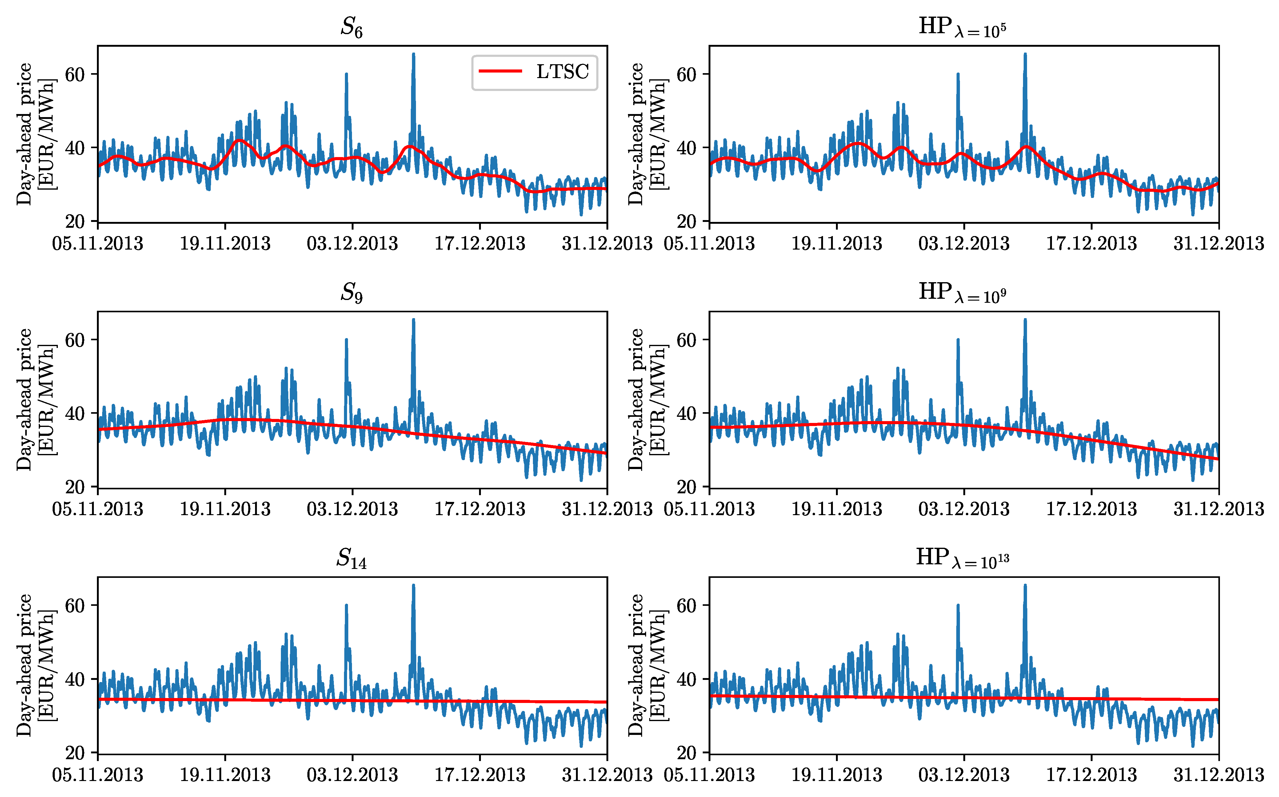We consider the Daubechies family of wavelets, which is frequently used in EPF studies [8,9,10,11,36,37,38,39]. More precisely, we utilize Daubechies wavelets of order 4 (that are denoted by ‘db4’), and the smoothing level k ranges from 6 to 14. Readers are directed to the left panels in Figure 3 for an illustration.

While wavelet smoothing removes layers of details, $D_1$, $D_2$, etc., the Hodrick–Prescott [40] filter simply returns $T_t$, which minimizes squared deviations from $Y_t$ (first term) and squared fluctuations of the smoothed series itself (the second term):

$$\underset{T_t}{min}\left\{\sum _{t=t_0}^{\tau }{(Y_t-T_t)}^2+\lambda \sum _{t=t_0+1}^{\tau -1}{\left[(T_{t+1}-T_t)-(T_t-T_{t-1})\right]}^2\right\},$$

(6)

where $t_0$ and $\tau$ are, respectively, the beginning and end of the calibration window in the single time index notation, and $\lambda$ is the smoothing parameter. Here, we consider nine values of the latter: $\lambda ={10}^k$ with $k=5,6,\dots ,13$. The larger the $\lambda$, the smoother the resulting series, see the right panels shown in Figure 3.

3.3. The OLS-Estimated Benchmark

As a benchmark, we consider the well-performing ${\mathrm{expert}}_{\mathrm{DoW},\mathrm{nl}}$ model that was proposed in [15], which was extended to include two exogenous variables. We denote it by ARX to reflect its autoregressive structure with exogenous variables. Within this model, the transformed price on day d and hour h is given by:

$$\begin{array}{cc}\hfill X_{d,h}=& \underset{\text{autoregressive effects}}{\underbrace{{\beta }_{h,1}{X}_{d-1,h}+{\beta }_{h,2}{X}_{d-2,h}+{\beta }_{h,3}{X}_{d-7,h}}}+\underset{\text{non-linear effects}}{\underbrace{{\beta }_{h,4}{X}_{d-1,min}+{\beta }_{h,5}{X}_{d-1,max}}}+\underset{\text{midnight value}}{\underbrace{{\beta }_{h,6}{X}_{d-1,24}}}\hfill \\ & +\underset{\text{exogenous variables}}{\underbrace{{\beta }_{h,7}{C}_{1,d,h}+{\beta }_{h,8}{C}_{2,d,h}}}+\underset{\text{weekday dummies}}{\underbrace{\sum _{i=1}^7{\beta }_{h,8+i}{D}_{i,d}}}+{ϵ}_{d,h},\hfill \end{array}$$

(7)

where $X_{d-1,min}$ and $X_{d-1,max}$ are the previous day’s minimum and maximum observations, $X_{d-1,24}$ is the previous day’s midnight value, i.e., the last known observation in the day-ahead market, $C_{1,d,h}$ and $C_{2,d,h}$ are two exogenous variables (here, day-ahead forecasts of price drivers that are relevant for a given dataset, see Section 2), $D_{1,d},\dots ,D_{7,d}$ are weekday dummies, and ${ϵ}_{d,h}$ is the noise term. The parameters of the model are estimated using OLS, independently for each hour.

3.4. The LEAR Model

The structure of the main predictive model that is considered in this study is a natural extension of Equation (7), which includes all 24 hourly observations for the considered three days, i.e., yesterday, two days ago, and a week ago, and predictions of the exogenous variables for all 24 h of the day:

$$\begin{array}{cc}\hfill X_{d,h}=& \sum _{i=1}^{24}\left({\beta }_{h,i}{X}_{d-1,i}+{\beta }_{h,24+i}{X}_{d-2,i}+{\beta }_{h,48+i}{X}_{d-7,i}\right)+{\beta }_{h,73}{X}_{d-1,min}+{\beta }_{h,74}{X}_{d-1,max}\hfill \\ & +\sum _{i=1}^{24}\left({\beta }_{h,74+i}{C}_{1,d,i}+{\beta }_{h,98+i}{C}_{2,d,i}\right)+\sum _{i=1}^7{\beta }_{h,122+i}{D}_{i,d}+{ϵ}_{d,h}.\hfill \end{array}$$

(8)

We estimate the 129 regressors via the least absolute shrinkage and selection operator (LASSO) [41]:

$${\widehat{\beta }}_h=\arg \underset{\beta }{min}\left(\mathrm{RSS}+\alpha \sum _{i=1}^{129}{\beta }_{h,i}\right),$$

(9)

where RSS is the residual sum of squares and $\alpha \ge 0$ is a tuning parameter. For $\alpha =0$, we get the standard OLS estimator, for large values of $\alpha$, all coefficients become zeros, while, for intermediate $\alpha$’s, the LASSO shrinks some of them to zero and, thus, performs variable selection. There are several techniques for optimizing the tuning parameter [42]. Here, we use cross-validation with seven folds since the number of observations in the calibration window is divisible by 7. Following [21], we refer to this LASSO-estimated autoregressive model as the LEAR model, although the LEAR model that is defined in [21] is a richer structure (it includes nearly 250 regressors, most notably lagged fundamental variables).

3.5. Forecast Averaging Schemes

The best-performing seasonal decomposition is not known in advance. We utilize forecast averaging to address this problem [28,29,30]. We generate a pool of forecasts from a single model (here, ARX or LEAR) calibrated to data decomposed with different filters (either wavelet- or HP-based) and then combine them into a single value, as suggested in [8]. We consider two methods of combining point forecasts—one that selects the best combination of a pool of models and one that is inspired by Bayesian Model Averaging [27].

Moreover, because our results (see Section 4) do not provide a clear indication for the optimal order of applying transformations—seasonal decomposition first and variance stabilization second, i.e., VST[SD(×)], or variance stabilization first and seasonal decomposition second, i.e., and SD[VST(×)]—we also consider combining the forecasts from both approaches. Overall, the combined predictions are constructed from individual forecasts: either 18 wavelet-based (nine smoothing levels and two orders of applying transformations) or 18 HP filter-based (nine values of $\lambda$ and two orders of applying transformations).

3.5.1. Best Combination

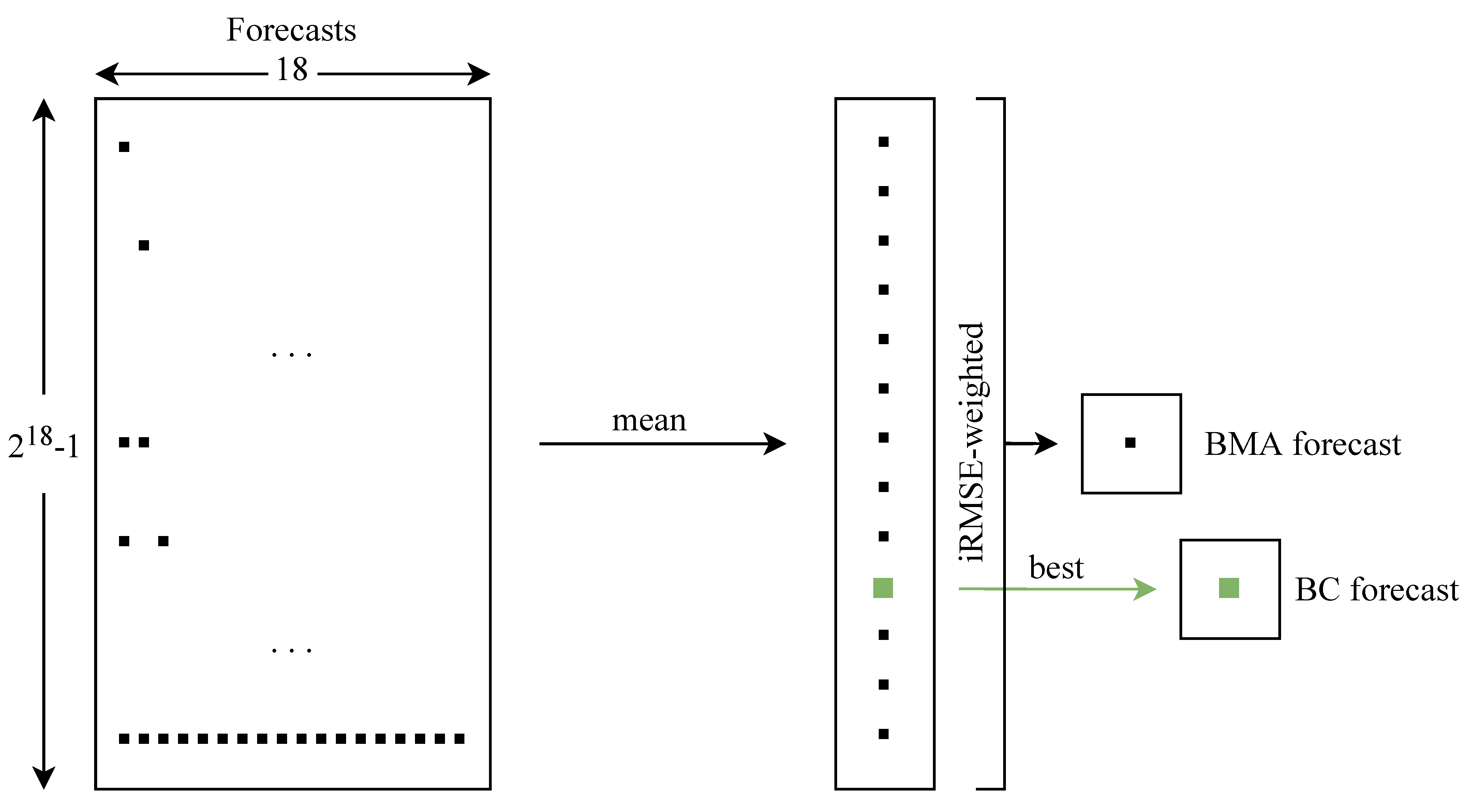
The simpler averaging scheme selects the best performing combination of a pool of models. Hence, we refer to it as the Best Combination and denote it by BC. Overall, given 18 individual forecasts (→ columns in the left rectangle in Figure 4), there are $2^{18}-1$ possible combinations (→ rows in the same rectangle). The first combination is just the forecast for the first LTSC, the second is the forecast for the second LTSC, …, the 19th is the combination of forecasts for the first and second LTSCs, the 20th is the combination of forecasts for the first and third LTSCs, …, and the last is the combination of forecasts for all of the LTSCs.

In each row, the predictions are averaged using the arithmetic mean. Subsequently, in order to choose the best-performing combination, we calculate the root mean squared error (RMSE) for all considered combinations of forecasts in the model selection window (i.e., the two-year period directly preceding the three-year test period, see Figure 1 and Figure 2):

$$\mathrm{RMSE}=\sqrt{\frac{1}{728\times 24}\sum _{d=365}^{1092}\sum _{h=1}^{24}{(p_{d,h}-{\widehat{p}}_{d,h}^c)}^2},$$

(10)

where ${\widehat{p}}_{d,h}^c$ is one of the $2^{18}-1$ combined forecasts and $p_{d,h}$ is the actual price for day d and hour h. We choose the combination that returns the lowest RMSE, as seen in the green square in Figure 4. This combination is eventually evaluated in the model evaluation window (i.e., the three-year test period) and compared to other combined and individual models.

In

Table 2. Root mean squared errors (RMSE) and their inverse values (iRMSE) calculated in the two-year model selection window (see Figure 1 and Figure 2) for the five best-performing combined forecasts obtained from the LEAR models with wavelet-based filtering. Squares indicate individual forecasts that are averaged in a given combination. For comparison, the last row represents averaging over all individual forecasts. Individual models where seasonal decomposition is executed first, and then the VST is applied, are labeled by VST[SD(×)], whereas models with the opposite order are labeled by SD[VST(×)].

Nord Pool market

VST[SD(×)]

SD[VST(×)]

$S_6$

$S_7$

$S_8$

$S_9$

$S_{10}$

$S_{11}$

$S_{12}$

$S_{13}$

$S_{14}$

$S_6$

$S_7$

$S_8$

$S_9$

$S_{10}$

$S_{11}$

$S_{12}$

$S_{13}$

$S_{14}$

$\mathrm{RMSE}$

$\mathrm{iRMSE}$

1

▪

▪

▪

▪

2.2984

0.4351

2

▪

▪

▪

2.2984

0.4351

3

▪

▪

▪

2.2985

0.4351

4

▪

▪

▪

▪

2.2991

0.4350

5

▪

▪

▪

▪

2.3002

0.4347

▪

▪

▪

▪

▪

▪

▪

▪

▪

▪

▪

▪

▪

▪

▪

▪

▪

▪

2.3485

0.4258

PJM market

VST[SD(×)]

SD[VST(×)]

$S_6$

$S_7$

$S_8$

$S_9$

$S_{10}$

$S_{11}$

$S_{12}$

$S_{13}$

$S_{14}$

$S_6$

$S_7$

$S_8$

$S_9$

$S_{10}$

$S_{11}$

$S_{12}$

$S_{13}$

$S_{14}$

$\mathrm{RMSE}$

$\mathrm{iRMSE}$

1

▪

▪

▪

19.0596

0.0525

2

▪

▪

▪

19.1281

0.0523

3

▪

▪

▪

19.1423

0.0522

4

▪

▪

▪

19.1633

0.0522

5

▪

▪

▪

▪

▪

19.2004

0.0521

▪

▪

▪

▪

▪

▪

▪

▪

▪

▪

▪

▪

▪

▪

▪

▪

▪

▪

20.4995

0.0488

, we present the five best-preforming combinations in the model selection window that was obtained for both datasets and the LEAR model with wavelet-based filtering. Squares indicate individual predictions that are averaged in a given combination. For instance, for the NP dataset, the best combination is composed of forecasts for three LTSCs that were obtained by first applying seasonal decomposition, and then the VST: $S_8$, $S_{10}$, and $S_{13}$, and one LTSC being obtained by first applying the VST, then seasonal decomposition: $S_{10}$. The RMSE of this combination in the model selection window is 2.2984, being nearly the same as that of the second best combination. The last row in each part of the table represents averaging over all individual forecasts; for NP, the RMSE of 2.3485 is ca. 2% higher than the best-performing combination.

3.5.2. BMA-Type Averaging

The more complex averaging scheme, instead of selecting one forecast combination out of $2^{18}-1$ possibilities, weighs all of the combinations:

$${\widehat{p}}_{d,h}^{\mathrm{BMA}}=\sum _{i=1}^{2^{18}-1}{w}_i{\widehat{p}}_{d,h}^{c,i},$$

(11)

where ${\widehat{p}}_{d,h}^{c,i}$ is the ith of the $2^{18}-1$ combined forecasts. The weights are computed based on past performance:

$$w_i=\frac{{\mathrm{iRMSE}}_i}{{\sum }_{i=1}^{2^{18}-1}{\mathrm{iRMSE}}_i},$$

(12)

where ${\mathrm{iRMSE}}_i$ is the inverse of the root mean squared error of the ith combination in Equation (10), see Figure 4. In the last column of Table 2, we report iRMSE values for the five best-preforming combinations that were obtained for both datasets and the LEAR model with wavelet-based filtering. As can be seen, because of the small differences in RMSE values, the weights are nearly identical for the top performing combinations and very similar to the weight for the average across all individual forecasts.

This idea is similar in spirit to Bayesian Model Averaging [27], which weighs combinations by posterior probabilities. The latter has not performed very well in an extensive EPF study [30], thus inspiring our idea to replace posterior probabilities by iRMSE weights, similarly to what was done in [28,29]. Although our approach is only inspired by Bayesian Model Averaging, for simplicity of notation, we denote it by BMA.

4. Results

4.1. Forecast Evaluation

Forecast accuracy is assessed in the three-year or $3\times 364=1092$-day model evaluation window, using two error measures. Following the recommendations put forward in [21], both are relative metrics. This allows us to compare the model performance across different datasets. The relative mean absolute error (rMAE) and the relative root mean squared error (rRMSE) are defined as:

$$\mathrm{rMAE}=\frac{{\sum }_{d=1093}^{2184}{\sum }_{h=1}^{24}\left|p_{d,h}-{\widehat{p}}_{d,h}\right|}{{\sum }_{d=1093}^{2184}{\sum }_{h=1}^{24}\left|p_{d,h}-{\widehat{p}}_{d,h}^{\mathrm{naive}}\right|},\mathrm{rRMSE}=\frac{\sqrt{{\sum }_{d=1093}^{2184}{\sum }_{h=1}^{24}{\left(p_{d,h}-{\widehat{p}}_{d,h}\right)}^2}}{\sqrt{{\sum }_{d=1093}^{2184}{\sum }_{h=1}^{24}{\left(p_{d,h}-{\widehat{p}}_{d,h}^{\mathrm{naive}}\right)}^2}},$$

(13)

where $p_{d,h}$ denotes the actual (observed) price for day d and hour h, ${\widehat{p}}_{d,h}$ is the corresponding prediction that is obtained using the model under the evaluation, and ${\widehat{p}}_{d,h}^{\mathrm{naive}}$ is a similar-day prediction [43]:

$${\widehat{p}}_{d,h}^{\mathrm{naive}}=\left\{\begin{array}{cc}{p}_{d-7,h}\hfill & \mathrm{for}\mathrm{Monday},\mathrm{Saturday},\mathrm{and}\mathrm{Sunday},\hfill \\ p_{d-1,h}\hfill & \mathrm{otherwise}.\hfill \end{array}\right.$$

(14)

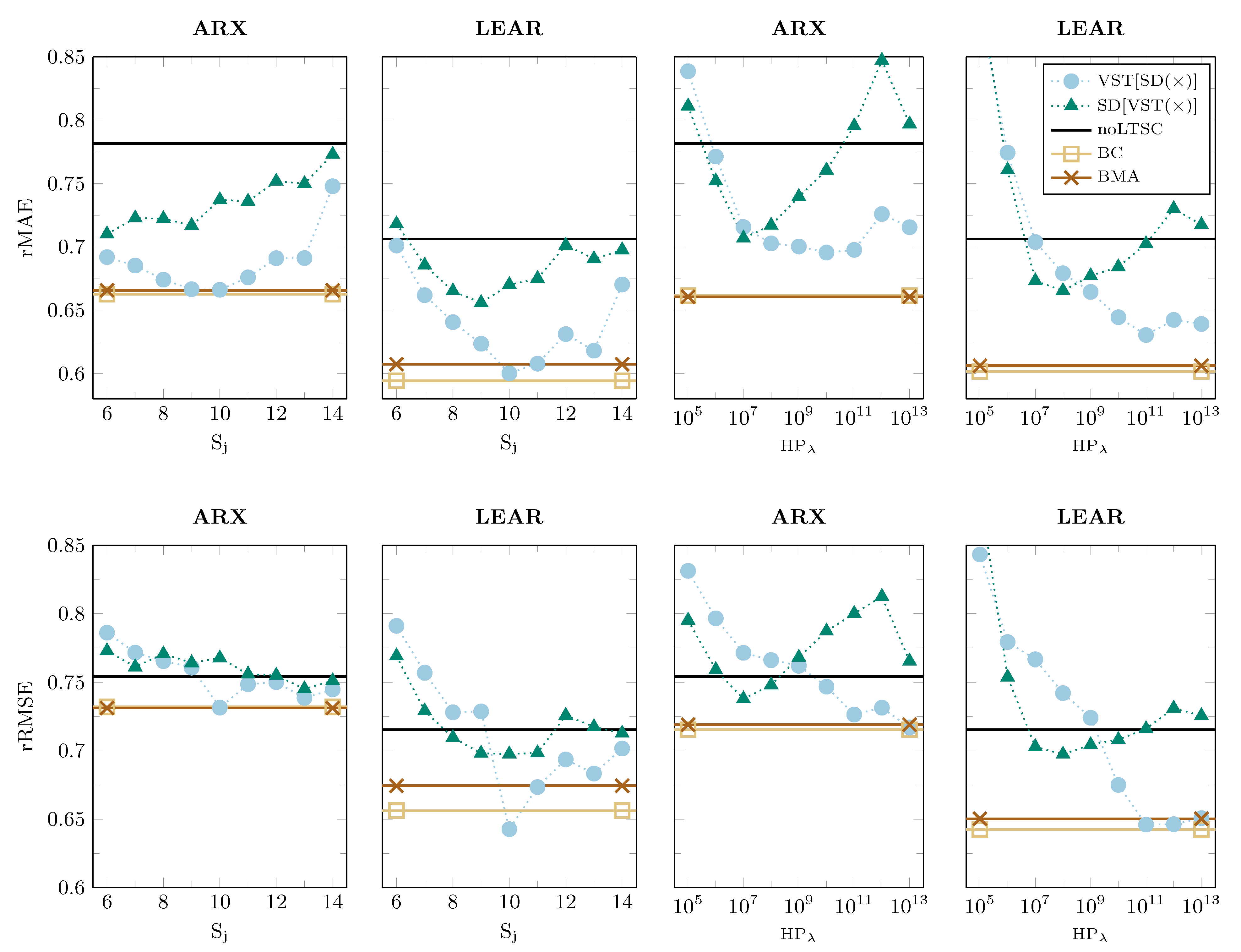
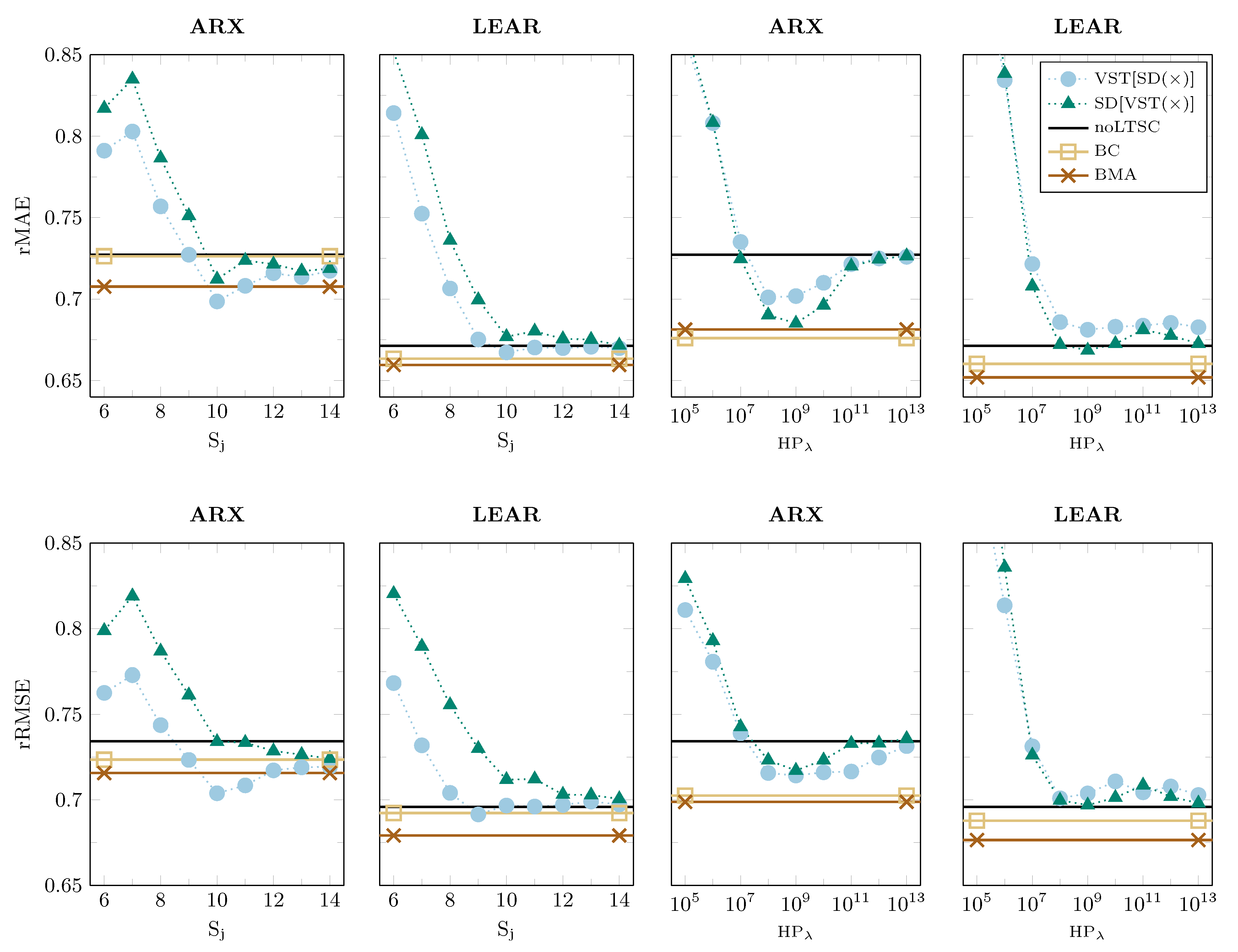
Figure 5 and Figure 6 present the results for the individual and combined ARX and LEAR models for both datasets. They all lead to similar conclusions.

Firstly, we can see that seasonal decomposition can improve the accuracy of forecasts that are generated not only by simple autoregressive models, but also by parameter-rich models with automated variable selection via the LASSO. More considerable improvements can be achieved in the NP market, see Figure 5. Moreover, in this case, most of the individual models with seasonal decomposition return lower error scores than the benchmark model without it (as denoted by noLTSC). For the PJM dataset, the improvements are smaller, and they occur more frequently for ARX models, as seen in Figure 6. The only problem with such individual models is that not all of them beat the benchmark model without seasonal decomposition. Thus, it is difficult to choose the optimal LTSC ex-ante.

Secondly, there is no general answer to the question of which order of applying data transformations performs better. It seems to depend on the considered model, market, type of the LTSC, or error measure. For instance, in the top row of Figure 6, where the rMAE is presented for the PJM dataset, the best performing approach changes depending on the filtering type considered. For wavelet-based filters, it is generally more effective to apply the seasonal decomposition first, whereas, for HP-based filters, the is best applied VST first. On the contrary, for the NP dataset and rRMSE (see the bottom row of Figure 5), the performance strongly depends on the chosen parameters that are used to extract the LTSC, i.e., the smoothing level k or the smoothing parameter $\lambda$.

We consider two averaging schemes to overcome these difficulties, see Section 3.5. In

Table 3. The relative mean absolute errors (rMAE) and relative root mean squared errors (rRMSE) calculated in the model evaluation window for the combined and the baseline ARX and LEAR models. The lowest score in a row is emphasized in bold, independently for the ARX and LEAR models, whereas the lowest score in a row across all of the models has a green background.

Error	ARX				LEAR
	noLTSC	LTSC	BC	BMA	noLTSC	LTSC	BC	BMA
Nord Pool market
rMAE	0.7817	HP	0.6615	0.6607	0.7062	HP	0.6016	0.6063
		db4	0.6626	0.6658		db4	0.5944	0.6074
rRMSE	0.7541	HP	0.7154	0.7190	0.7153	HP	0.6424	0.6503
		db4	0.7321	0.7312		db4	0.6563	0.6744
PJM market
rMAE	0.7273	HP	0.6761	0.6814	0.6713	HP	0.6603	0.6520
		db4	0.7263	0.7076		db4	0.6634	0.6596
rRMSE	0.7343	HP	0.7026	0.6988	0.6959	HP	0.6879	0.6765
		db4	0.7236	0.7157		db4	0.6923	0.6792

, we collect all of the error scores for the combined and benchmark models. It turns out that, for both datasets, the BC and BMA averaging schemes always return lower rMAE and rRMSE scores than the benchmark model without seasonal decomposition (denoted by noLTSC). Moreover, there are generally only a few individual models that can outperform the combined models. Hence, we can conclude that forecast averaging solves the problem with the ex-ante selection of the best performing LTSC and the order of data transformations. Furthermore, all of the combined LEAR models outperform their ARX counterparts, so the use of LASSO-estimated models additionally increases the accuracy of the combined forecasts.

Finally, let us compare the averaging schemes and the methods of modeling the LTSC. It turns out that the BMA approach returns lower errors than BC in nine out of 16 cases. When it comes to the best-performing approach for extracting the LTSC, we can observe that the one that is based on HP filters yields lower error scores in all of the cases except one (i.e., LEAR, BC averaging, NP market; see Table 3).

4.2. Testing for Conditional Predictive Ability

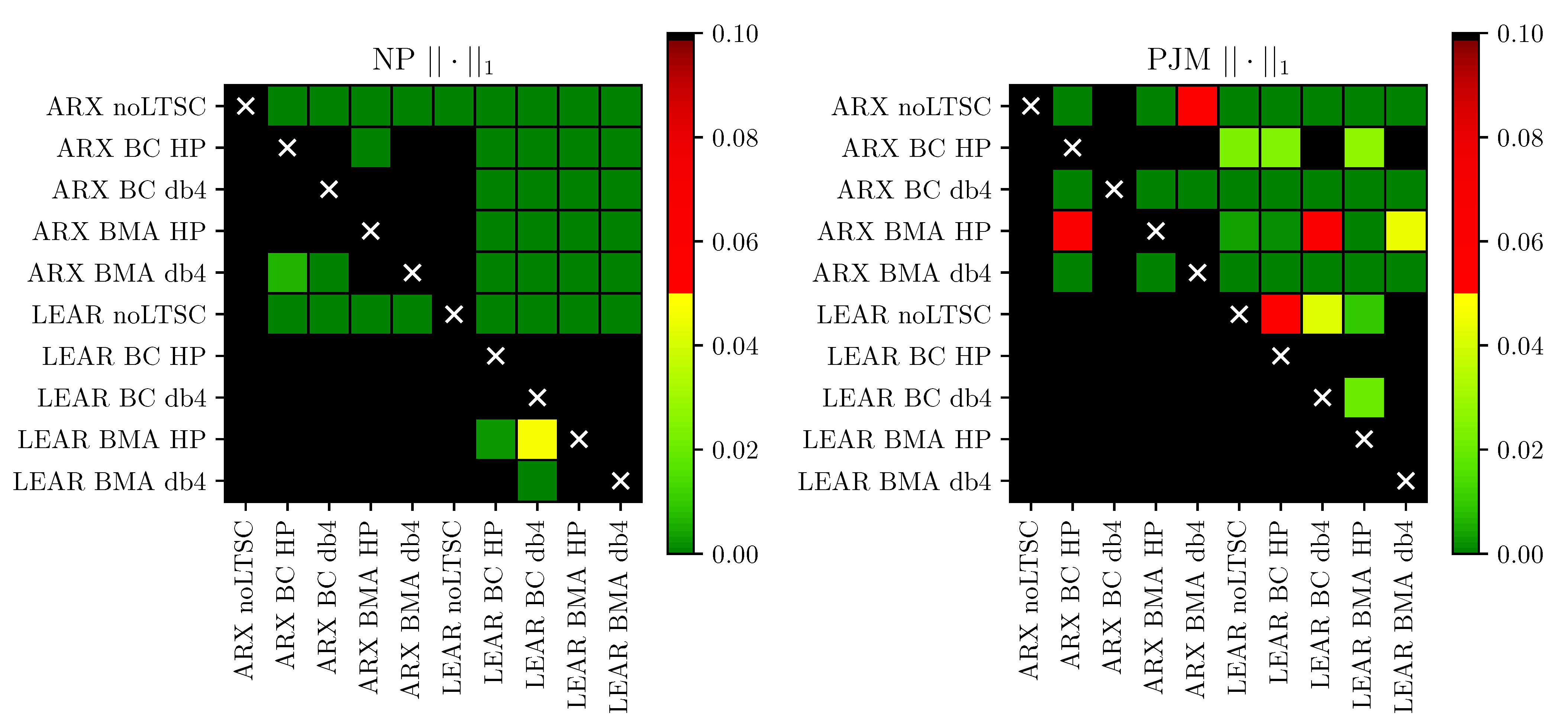
The obtained forecasts are also compared using the conditional predictive ability (CPA) test of Giacomini and White [32]. Here, following [15], we only focus on the results of the multivariate version of the test, which, for each pair of models, returns a single p-value for all 24 h. The tests were separately conducted for the absolute and squared losses.

Following [10,15,21], we present the CPA test results as chessboards with a color-coded p-value, where the color ranges from dark red (higher p-values) to dark green (lower p-values). A colored square in the chessboards indicates that the predictions of the model on the x-axis are significantly better than the predictions of the model on the y-axis. The greener this field (the lower the p-value is), the more statistically significant the difference. A black square means that there is no statistically significant difference in the predictive accuracy at the 10% level.

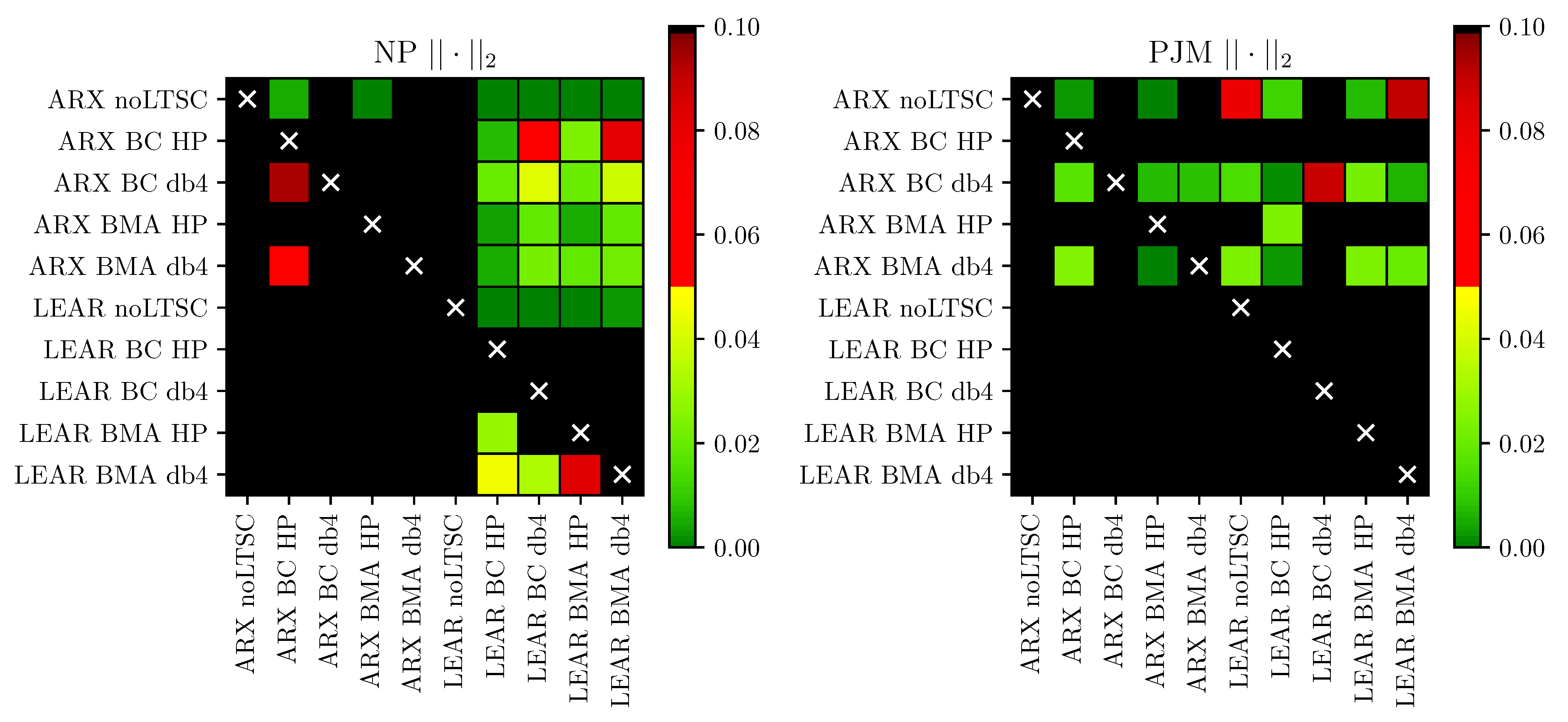
In Figure 7 and Figure 8, we illustrate the results for the absolute and squared losses, respectively. As can be seen, the combined forecasts significantly outperform the predictions of the benchmark models without seasonal decomposition in 22 out of 32 cases (at the 10% level). When we only consider the LEAR models, the improvement is statistically significant in 11 out of 16 cases. Only for the PJM market (both averaging schemes for the squared losses, see Figure 8, and LEAR BMA db4 for linear losses, see Figure 7), the improvements over the benchmark are not statistically significant. Moreover, the outperformance of the forecasts of the combined LEAR models over their ARX counterparts is significant in 14 out of 16 cases. Thus, the CPA tests confirm that seasonal decomposition improves the accuracy of combined forecasts that are generated by the LASSO-estimated models.

Regarding the method of combining forecasts, although the BMA approach returns lower errors than the BC approach in nine out of 16 cases (see Table 3), the CPA tests indicate that outperformance is only significant in two cases. On the other hand, the BC approach significantly outperforms the BMA approach in six cases. Given that the differences in the error scores between both of the averaging schemes are small, we can recommend the simpler approach—BC averaging.

Finally, although the combined models based on HP filters return lower error scores in almost all cases, the advantages of using one LTSC function over the other are not so clear from the perspective of the CPA test. The combined forecasts that are based on HP filters are only significantly better than those based on wavelet filters in six cases, at the 10% level, whereas the remaining 10 cases show no significant differences. When considering the 5% level and only the combined LEAR models, all of the differences become statistically insignificant.

4.3. Computational Complexity

The models that are considered in this study are computationally feasible, even in time-constrained scenarios. It is notable that all of the times reported in this subsection reflect a single-threaded task run on an AMD Threadripper 1950X processor.

The average computation time per forecast day amounts to 8–9 s for the LEAR models and 0.03–0.05 s for the ARX models. The listed times reflect the whole process, including data preprocessing, such as the application of the LTSC or the VST. Nevertheless, model estimation is the most time-consuming task. To be more precise, the ARX model without the LTSC is, on average, computed in 0.027 s, whereas the computation of the same model with the LTSC takes 0.03 s for db4 wavelets and 0.05 s for HP filters. For the LEAR model, the input data impact the convergence rate. The smallest time in this case was measured for the model with the LTSC based on db4 wavelets—8 s per day. On the other hand, for the model with the LTSC that was based on HP filters or without the LTSC, the computations took closer to 9 s.

The averaging schemes require additional computational time. One has to consider the generation of forecasts to determine the best averaging scheme. The sequential computation of the set of forecasts for one LTSC variant and a 728-day selection window takes around 33 h. Computing the errors of all $2^{18}-1$ possible combinations of the forecasts takes 101 s. However, the above operations are only done once.

5. Conclusions

To address the question of whether the seasonal component approach is beneficial in the case of parameter-rich models, we have performed an extensive empirical study that involved a well-performing, LASSO-estimated autoregressive (LEAR) model with 129 regressors, two approaches to modeling the LTSC (wavelet smoothing and the Hodrick-Prescott filter), and the area hyperbolic sine transformation. Given that our initial results did not provide a clear indication for the optimal choice of the LTSC or the optimal order of applying transformations—seasonal decomposition first and then variance stabilization second, or vice versa—we have introduced two averaging schemes. The first one, dubbed Best Combination (BC), selects the best combination of a pool of models. The second is inspired by Bayesian Model Averaging, but it weighs combinations by the inverse (of the) root mean squared error (iRMSE), instead of the originally proposed posterior probabilities; for notational convenience, we refer to it as BMA.

Our results indicate that seasonal decomposition can significantly—as measured by the conditional predictive ability (CPA) test—improve the accuracy of the forecasts that are generated not only by simple autoregressive, but also by parameter-rich models with automated variable selection via the LASSO. Moreover, for both datasets, the averaging schemes always return lower error scores than the benchmark model without seasonal decomposition. At the same time, there are only a few individual models that can outperform the combined models. Hence, we can conclude that forecast averaging solves the problem with the ex-ante selection of the best performing LTSC and order of data transformations. Furthermore, all of the combined LEAR models outperform their parsimonious ARX counterparts, so the use of LASSO-estimated models additionally increases the accuracy of the combined forecasts. Although the BMA approach generally returns slightly lower errors than BC, the CPA tests indicate that outperformance is, in most cases, insignificant. Hence, we recommend the simpler approach—BC averaging. Interestingly, this is consistent with the recommendations put forward in the forecasting literature, i.e., that instead of combining the full set of forecasts, it may be advantageous to discard the models with the worst performance [29,44].

Finally, let us note that forecasts, no matter how accurate, are of limited use if they cannot be utilized to yield profits [16]. However, measuring the economic value of reducing electricity price forecasting errors—although desirable—is a difficult task, as argued in [45,46]. A model that yields lower errors may not always lead to better trading decisions. Because there are no golden standards in this respect, instead of devising an artificial strategy, we encourage practitioners to evaluate our models in an actual trading environment. Our codes are available upon request.