Article

Predictive Trajectory Control with Online MTPA Calculation and Minimization of the Inner Torque Ripple for Permanent-Magnet Synchronous Machines

Institute of Electrical Engineering (ETI), Karlsruhe Institute of Technology (KIT), Kaiserstr. 12, 76131 Karlsruhe, Germany
*
Author to whom correspondence should be addressed.
Energies 2020, 13(20), 5327; https://doi.org/10.3390/en13205327
Submission received: 27 August 2020 / Revised: 25 September 2020 / Accepted: 12 October 2020 / Published: 13 October 2020
(This article belongs to the Special Issue Permanent Magnet Electrical Machines)

Abstract

:
This paper presents an extended predictive trajectory control scheme combined with an inner torque ripple minimization considering the current-, flux-linkage-, and voltage-planes of permanent magnet synchronous machines. The extension of a fundamental machine model with flux-linkage harmonics allows the calculation of the inner torque ripple and enables its minimization. For this, the control is divided in two cases: (1) The dynamic operation or large signal behavior which uses the maximal torque gradient for the trajectory strategy during each control period for fastest dynamic operation, and (2) The stationary operation or small signal behavior, utilizing a real time capable polynomial approximation of the rotor position dependent torque hyperbolas (iso-torque curves) of permanent magnet synchronous machines for the ideal torque to current reference values. Since dynamic and steady-state operation is covered, torque to current look-up tables, such as maximum torque per ampere (MTPA)/maximum torque per volt/voltage (MTPV) look-up tables, are not required anymore. The introduced, new control approach is implemented in Matlab/Simulink based on finite element analysis and measured data. Furthermore, test-bench implementations based on measurement data are presented to show the real-time capability and precision.

Graphical Abstract

1. Introduction

The calculation of the ideal reference values for permanent magnet synchronous machine (PMSM) control is still intensively investigated [1]. Today’s control algorithms for PMSMs are mostly direct torque control (DTC) or field oriented control (FOC) algorithms. Both require precalculated torque dependent reference values for the control. In case of the DTC flux references are necessary and for FOC current references are necessary. In this paper only FOC approaches and therefore the current references are investigated. By calculating the maximum of the machine’s inner torque depending on the applied current magnitude the optimal reference values can be obtained. This method is called maximum torque per current (MTPC) or maximum torque per ampere (MTPA). At higher speed of the PMSM, in the field weakening operation, an optimization considering the voltage limit is mandatory. This principle is called maximum torque per volt/voltage (MTPV). Figure 1 shows the results of this basic MTPA and MTPV calculations.
Reference [2] gives a good overview over several basic methods. In addition, it describes and classifies the MTPA/MTPV methods and working principles. According to [2], the approach discussed in this paper can be classified as advanced, predictive online, model-based, and open loop torque control algorithm. A quite similar concept is described in [3], which also uses online estimation of the references by variation of the model parameters for only ideal fundamental reference torque.
However, not only the fundamental reference value calculation is an important issue in recent research, but also the calculation of precise torque references, which suppress additional torque oscillation due to spatial flux linkage harmonics. In the past, for this torque ripple suppression several possibilities were introduced. One of the methods is known as harmonic current injection (HCI). Its working principle are pre-calculated and/or optimized harmonic currents for each point of operation. This is calculated, mostly by using FEA (finite element analysis). These injected harmonic currents compensate, e.g., the cogging torque and/or the inner torque ripple which results in a smoother torque [4,5]. Quite similar to this, is the method described in [6]. Based on the identified machine parameters the MTPA/MTPV current references for smooth torque are pre-calculated and stored in lookup tables. These references are applied during regular FOC control. In [7] and [8] also an advanced PMSM model is used for the pre-calculation of the optimal currents or direct current trajectories for minimal torque ripple.

1.1. Motivation

The main contribution of this paper is an algorithm which calculates the optimal torque references at dynamic operation and minimizes the torque ripple at stationary operation, directly online. The novelty is the combination of both the compensating of the torque ripple and choosing the ideal dynamic torque trajectory during real time operation. The calculation of the necessary rotor position dependent references is challenging and often done offline due to their complexity. However, the online calculation enables possibilities of adaptable torque references even when the machines parameters vary during operation caused by rotor temperature, faults or aging effects, which can be detected and adopted, e.g., by online identification algorithms.
In the presented approach, with the predictive trajectory control scheme from [9], based on the necessary underlying flux-linkage and inverse fundamental current-lookup tables, is used and further extended for a predictive and direct calculation of the torque references at dynamic and steady-state operation considering the harmonic behavior. Furthermore, the suppression of torque harmonics is enabled considering the estimated rotor position and current dependent PMSM.

1.2. Preliminary Work

The introduced algorithm is based on the predictive trajectory current control scheme introduced in [9] and extended with a new rotor position dependent model. The new control scheme uses thereby precise test bench identified fundamental flux-linkage models parameterized with measured data. By considering the available control voltage in every time step, each operational point yields individual limited system values. The limited values are separated and visualized as different, so-called rotor position dependent system-planes, the flux-linkage plane, the current plane, and the voltage plane. For dynamic and stationary control, two different cases are distinguished. First, the current reference value is reachable which yields directly solvable nonlinear voltage equations. Second, the current reference is not reachable within one control period and has to be limited. In this case, the optimization of the limitation and the trajectory planning for the connection of the latest current to the reference current value is calculated. The introduced approach extends this principle by the online calculation of reference currents and by considering position-dependent flux-linkages for a smooth torque.

1.3. Outline of the Paper
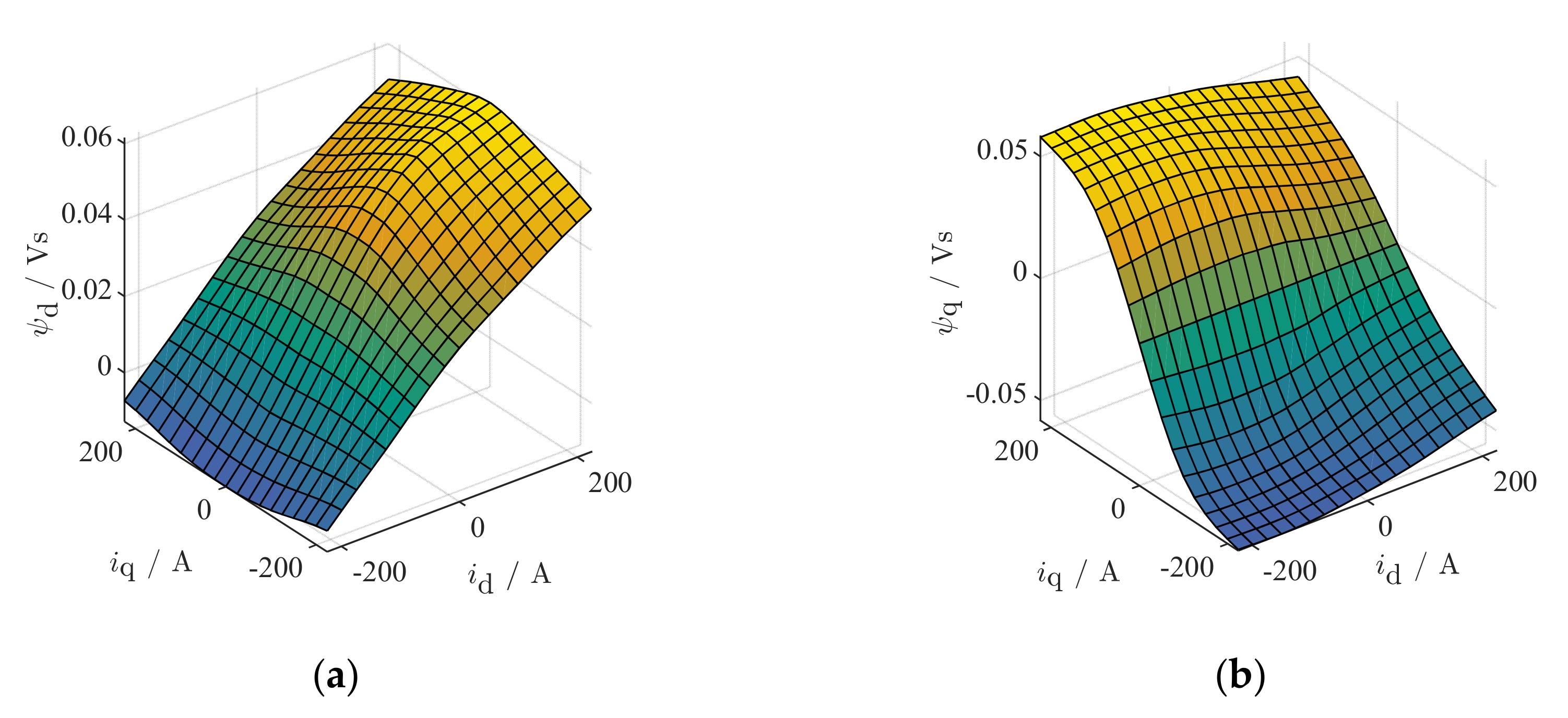
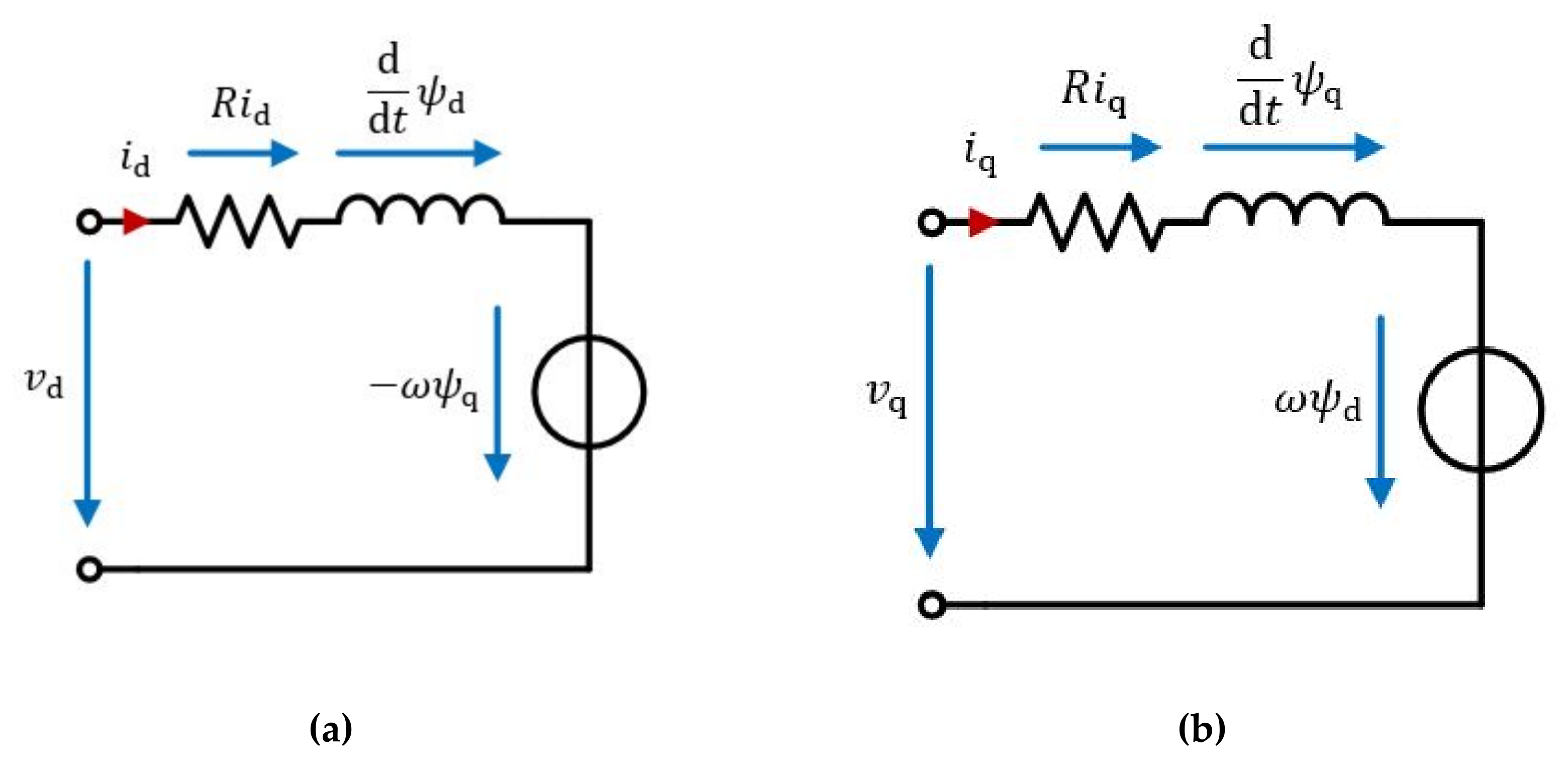
First, in Section 2 the necessary time-continuous and time-discrete machine model with position dependent flux-linkages and the resulting inner torque are introduced. Furthermore, the test bench identification of the flux-linkages is briefly introduced (see Section 2.2). The control algorithm is derived for dynamic (Section 3.3.1) and steady-state operation (Section 3.3.2). After the explanation of the test setup, first simulation (Section 3.4) and measurement results (Section 5) are shown. The paper concludes with a discussion of some simulation and measurement results in Section 6.

2. Machine Model

In this section the necessary dq-model equations, assumptions and the principle of flux-linkage parameter identification are described. These model equations and its parameters form the basis of the control algorithm derived in the next section. For usage within time-discrete systems, the discretization of the model equations is also shown.

2.1. Permanent Magnet Synchonous Machine Model

The model equations of the equivalent circuit are derived from the known three-phase model equations. We assume three symmetric stator windings. For simplification, the friction as well as the iron losses are neglected. Furthermore, dielectric currents, thermal, skin, and proximity effects are not considered. The machine’s three-phase stator voltage equations are derived from Ohm’s law, Kirchhoff’s law, and the Maxwell equations. Park-transformation of the three phase system provides the rotor-oriented dq0-reference frame and thus the Equations (1)–(3), [10,11].
The ohmic resistance of the stator windings is R , the electric angular frequency is ω . The voltage, flux-linkage, and current components of the direct-axis, quadrature-axis, and zero-axis are ψ x , v x   and i x with x d , q , 0 .
v d   =   R i d   +   d d t ψ d ω ψ q
v q   =   R i q   +   d d t ψ q   +   ω ψ d
v 0   =   R i 0   +   d d t ψ 0 ,
The torque of the electrical machine can be derived from the power balance of mechanical and electrical power as shown in [10]. In the Equation (4) for the power is shown. T denotes the inner torque of the machine, p is the number of pole pairs. The inner torque is assumed to be the shaft torque neglecting the magnetic stray/leakage flux (which causes, e.g., the cogging torque) and the friction losses, [8,12].
T ω p   =   3 2 R i d 2   +   i q 2   +   2 i 0 2   +   ω ψ d i q ψ q i d   +   i d d d t ψ d   +   i q d d t ψ q   +   2 i 0 d d t ψ 0 ,
In this case, the machine is assumed to be star-connected. Therefore, there is no zero-sequence current and the zero sequence dependent terms of the inner torque are disappearing in the following. The dq-equivalent circuit model layout is shown in Figure 2.
Assuming that the ohmic losses do not affect the torque, the stator resistance dependent terms are ignored. The partial derivatives for the total derivative d d t ψ dq of the flux-linkages ψ dq   =   f i d , i q , γ considering the variables i d , i q , γ yield the expression of the differential inductances. The partial derivatives are   L dd d i d d t , L dq d i d d t , L qq d i q d t , L qd d i q d t and the derivative considering γ are   ψ d γ d γ d t and ψ q γ d γ d t .
Assuming that the differential inductances are only part of the inner magnetic power of the machine and do not couple into the inner torque. Only the term γ d γ d t ψ dq is considered for the extended torque equation. At constant speed (which is assumed in this paper) the derivative of the electric angle γ is the electric angular velocity d γ d t   =   ω . The resulting, simplified equation for the inner torque is (5). The factor 3 2 is due to the amplitude invariant transformation [10]. The term ψ d i q ψ d i q describes the fundamental torque, i d ψ d γ   +   i q ψ q γ is the dynamic torque term caused by rotor revolution. The flux-linkages are modelled by a function ψ dq   =   f i d , i q , γ . This yields the simplified inner torque Equation (5).
T   =   3 2 p ψ d i q ψ q i d   +   i d ψ d γ   +   i q ψ q γ ,
The necessary flux-linkages for the equation can be identified either by simulation (e.g., finite element analysis, FEA) or by measurement. Due to manufacturing influences and additional parasitic effects, which are not always considered in FEA, in this case the measured flux-linkages are preferred. The test-bench identification of the rotor-position and current dependent flux-linkage is a challenging task and will be shortly described in the following section.

2.2. Parameter Identification

The identification of the stator-resistance R is done by four-terminal sensing at balanced thermal condition. The, for the control, necessary flux-linkages can be identified are identified by test-bench measurement as explained in the following. For the test-bench flux-linkage identification there are certain requirements. At first the load machine has to be controlled at constant rotational speed. Enough inertia of the test-bench is helpful to ensure this requirement. Second, the device under test machine has to be ideally current controlled to ensure ideal constant dq-currents. A possible control algorithm in this case, with mitigation of the current harmonics, is described in [13]. The pre-initialization of this model based control, with current harmonic mitigation, can be done with approximated fundamental flux-linkages or first FEA results. Measuring the voltages u d , u q at various operating points with evenly distributed i d , i q currents at constant rotational speed enables the calculation of the flux-linkages.
For the solution of the resulting coupled differential Equations (6) and (7) the “separation of the variables” method is used [14].
v d   =   R i d   +   ψ d γ d γ d t ω ψ q i d
v q   =   R i q   +   ψ q γ d γ d t   +   ω ψ d i q ,
The voltage time-series is rewritten as a Fourier series (8); thereby, ρ denotes the order of the investigated harmonic frequency in the dq-reference frame.
v dq t   =   v dq 2 ¯   +   ρ   =   1 N 2 v dq , a , ρ cos ω ρ t   +   v dq , b , ρ sin ω ρ t ,
The general solution y of the differential equation is y = y c   +   y p . Equation (9) shows the particular integral y p , which is the trivial solution of this differential equation. The variables of y p are time-invariant.
ψ ¯ d ψ ¯ q = 1 ω 0 1 1 0 v ¯ d v ¯ q R i d i q ,
The complementary function   y c   includes only the time-variant terms (10), the current or stator resistance dependencies are vanished.
v d , ρ t v q , ρ t = d d t ψ d , ρ t ψ q , ρ t   +   ω 0 1 1 0 ψ d , ρ t ψ q , ρ t ,
As the flux-linkage is the time-derivative of the voltages, the flux-linkage harmonics are of the same order as the voltage harmonics. The flux-linkages are interpreted as Fourier series analogous to the voltages. Insertion of both Fourier series simplifies Equation (10) to Equation (11). The Fourier series coefficients for the voltages are v dq , ab , ρ , as derived in (8), the coefficients for the flux-linkages are ψ dq , ab , ρ . The matrix V denotes the Fourier coefficients of the voltage, the matrix ψ denotes the Fourier coefficients of the flux-linkage. The matrix F describes the vector cos ω ρ t sin ω ρ t .
V F ω ρ t   =   d d t ψ F ω ρ t   +   ω 0 1 1 0 ψ F ω ρ t ,
After mathematical simplification, using the chain-rule and following solution of Equation (11), the Fourier series coefficients of the dq-flux-linkages can be calculated directly through the measured voltage coefficients as displayed in Equation (12).
I . ψ d , a , ρ   =   v q , a , ρ ρ v d , b , ρ ω ρ 2 1 II . ψ d , b , ρ = v q , b , ρ + ρ v d , a , ρ ω ρ 2 1 III . ψ q , a , ρ =   v d , a , ρ ρ v q , b , ρ ω ρ 2 1 IV . ψ q , b , ρ =   v d , b , ρ   +   ρ v q , a , ρ ω ρ 2 1 ,
With the flux-linkage coefficients   ψ dq , ab , ρ of the Fourier series for each harmonic ρ the flux-linkages ψ dq t at constant rotor speed ω and constant currents i dq can be established. This time-variant Fourier series can be discretized and stored rotor position dependent, considering γ t = ω t . The flux-linkages assumed now as ψ dq i d , i q , γ ω   =   const . . A more detailed view on the derivation of this parameterization approach, the assumptions, implementation, and measurement are presented in [14,15]. For example, the flux-linkages ψ d and ψ q of the prototype for the practical measurements, assuming ω   =   const . at a fixed rotor position γ is shown in Figure 3. The currents-planes i dq ψ d , ψ q , γ ω = const . , necessary for the control algorithm, can be calculated by numerical inversion of the flux-linkages ψ dq i d , i q , γ ω   =   const .

2.3. Time-Discrete Model Equations

Modern control algorithms are implemented on microprocessors. Thus, Equations (6) and (7) have to be time-discretized. Therefore, the trapezoidal rule is used for numerical integration. For the discretizing of the voltage equations further assumptions have to be taken. First, the electric frequency has to be assumed to be constant from the beginning t n to the end t n + 1 (with n ) of one control period T c . This is given if the inertia of the machine is sufficiently large enough. Second, it is assumed that the error, due to the flux-linkage linearization, within a short control period is negligible. The stator voltages can generally be expressed as (13) and (14), [9].
v d , t n , n + 1 = 1 2 R i d , t n   +   i d , t n + 1   +   ψ d , t n + 1 ψ d , t n T c 1 2 ω ψ q , t n   +   ψ q , t n + 1 ψ d , t n γ   +   ψ d , t n + 1 γ
v q , t n , n + 1 =   1 2 R i q , t n   +   i q , t n + 1   +   ψ q , t n + 1 ψ q , t n T c   +   1 2 ω ψ d , t n   +   ψ d , t n + 1 ψ q , t n γ   +   ψ q , t n + 1 γ ,
The in [9] introduced control scheme requires the conversion between the different so called system-planes, e.g., the conversion from the flux-linkages ψ dq as function of f ( i d , i q , γ ) = ψ d , ψ q , γ to the inverse flux-linkages i dq as function f 1 ψ d , ψ q , γ   =   i d , i q , γ . Therefore, the dynamic part of the ohmic voltage drop as well as the dynamic part of the voltage due to the position dependency of the flux-linkages have to be neglected for simplification of the calculations, (15) and (16). Which is admissible due to their mostly small influence.
v d , t n , n + 1   =   R i d , t n   +   ψ d , t n + 1 ψ d , t n T c 1 2 ω ψ q , t n   +   ψ q , t n + 1   +   ω ψ d , t n γ
v q , t n , n + 1   =   R i q , t n   +   ψ q , t n + 1 ψ q , t n T c   +   1 2 ω ψ d , t n   +   ψ d , t n + 1   +   ω ψ q , t n γ ,

2.4. Inverter- and Iron-Losses

The control algorithm derived in this paper is considered as a fully model-based approach. Due to the missing integral component of the control, every mismatch of the calculated reference voltage influences the torque output of the machine. Especially two major effects, which were neglected in the derivation of the model equations, influence this behavior. At first, the iron losses of the electrical machine which are mostly speed depended have to be considered for a full implementation. Second, the inverter and the wire loss have to be compensated for correct reference values.
Characterization of the machines iron-losses is possible, e.g., as described in [16]. The losses can be recalculated as voltage error and be applied at the respective operational point. Similar to the iron losses the inverter and wire losses can be calculated or identified also as voltage error between the reference voltage and the measured voltage at the machine terminals. The sum of the voltage errors due to iron losses and inverter losses can thus be described as a function g = u dq i d , i d , γ , ω , but this is not necessary for the principle of the control algorithm. For reasons of simplification, it is therefore neglected in this paper.

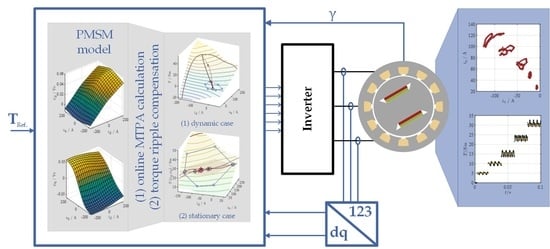
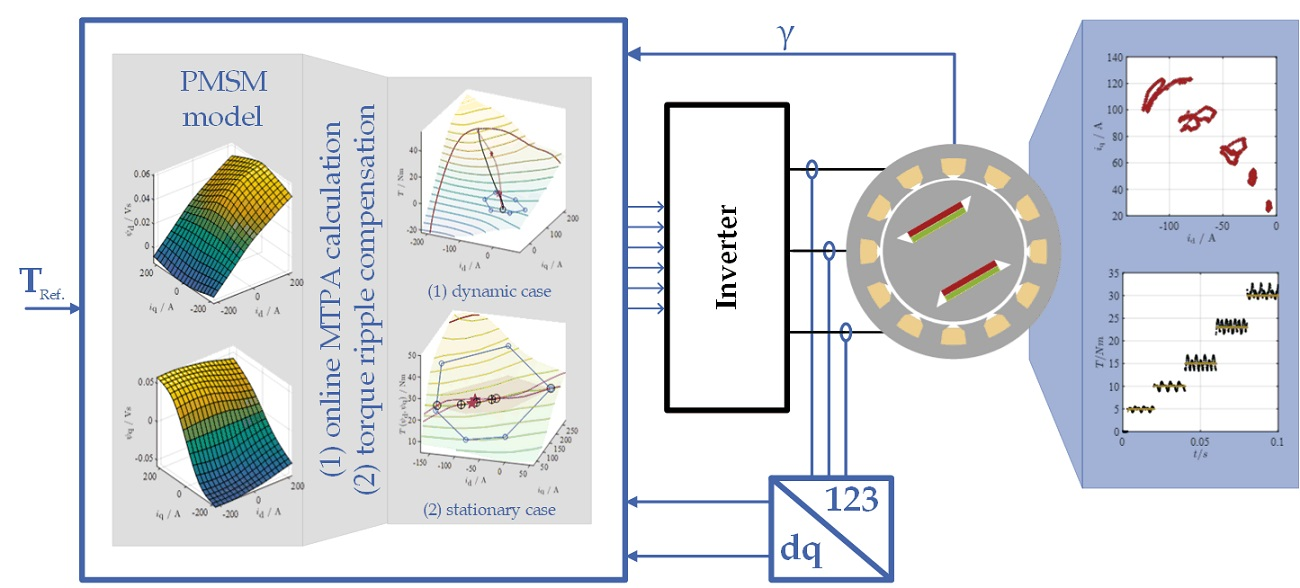
3. Control Algorithm

In the following section the principle of the algorithm is explained. The explanation and visualization of the trajectory-based algorithm is done using a virtual model with more distinct mutual and cross-saturation effects. At first the basic equations and principle of the predictive control according [9] are explained. Second the new algorithm and some simulation results are explained.

3.1. Simulation Environment

For the simulations and the visualization of the derived control algorithm, based on the physical parameters, a virtual test environment in Matlab/Simulink/Simscape from Mathworks has been set up. For a better understanding and explanation of the algorithm the simulation results are generated with a separately FEA build-up machine with distinct saturation effects, not with the later introduced test-bench used easier PMSM. This FEA build-up machine has more nonlinear effects as saturation and cross-saturation flux-linkages (Figure 3) which is useful, because the more challenging control behavior compared to the test-bench PMSM. The FEA data were generated with the software Flux2D from Altair.
The used virtual test environment enables rapid implementation, visualization, and development of control algorithms. The machine model equations are implemented in an acausal manner, which enables also analysis of the short circuit condition and examining the harmonic content of the induced voltage. The rotor speed in the simulation is utilized by an ideal constant source. In simulation, the inverter is modelled by means of equivalent dq-voltage sources. A description of the full machine behavior, based on FEA or measured data-sets, is thereby possible as described in [17].

3.2. Basic Principle of the Predictive Current Control

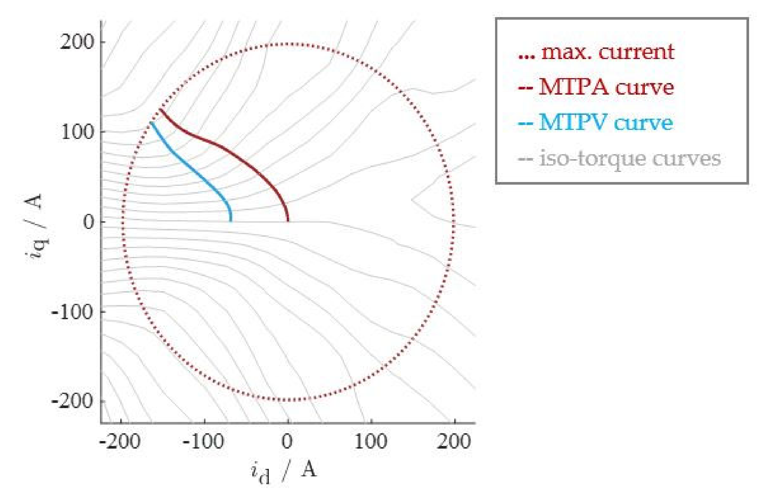
3.2.1. Operation Area Constraints

The drive system is limited due to physical conditions, which have to considered in the control algorithm. First, the thermal domain is limited by maximum current amplitude. The maximum current can be described as a circle with the radius of i max   =   i d 2   +   i q 2 . The maximum voltage has also to be bounded due to the limited DC-link. Second, the with the inverter reachable area can thus be described as voltage hexagon, with simplified linear connection of each of the six-corners, due to the six possible voltage phasors of the three phase two-level inverter. This voltage hexagon with the six corners v dq , j , t n with j 1 , 2 , 3 , 4 , 5 , 6 is depending on the actual operational point of the machine. For robust and stable control, especially at stationary operation, the voltage hexagon is shortened to its inner circle. This is necessary to reduce and simplify the calculation effort because of the rotor position dependent flux-linkage as well as the rotor position dependent voltage hexagon.

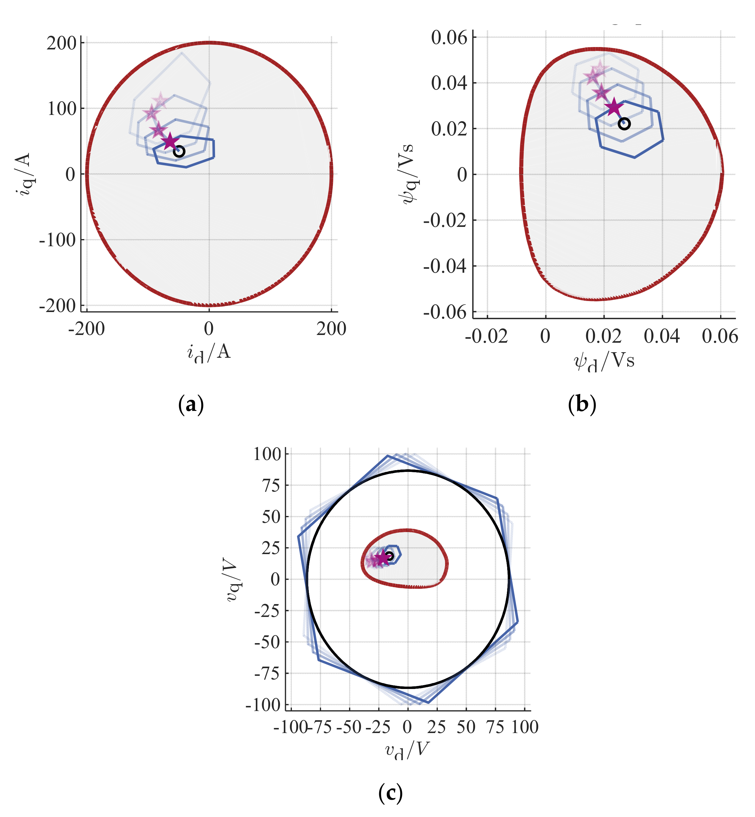
3.2.2. Current-, Flux-Linkage-, and Voltage-Planes

The algorithm is based on the visualization of the reachable operating points at the time t n + 1 considering the latest operating point t n within the different planes of the machine as shown in Figure 4. The evaluation of these planes enables the calculation of the ideal voltage references. The necessary procedure is motivated in the following.

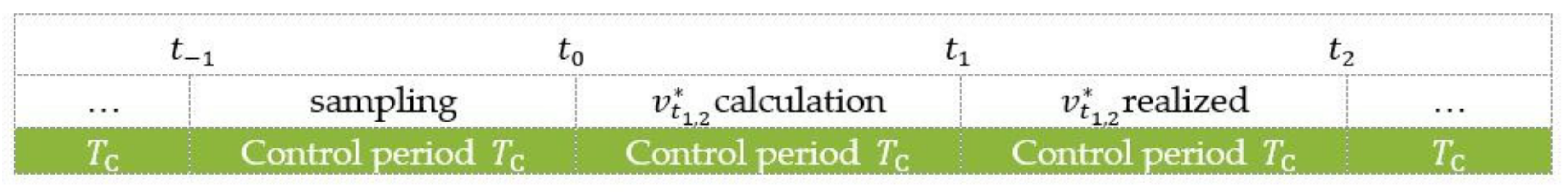
3.2.3. Timing of the Digital Control

In each sampling interval the predicted operating point, the reachable operating points and the reference values are calculated within the control procedure, Figure 5. To explain the chronological sequence of the calculations, t 0 is set as the current point in time. The time span (period) between t 1 and t 0 is therefore the sampling interval of the currents and rotor position. These values are allocated to the control at t 0 . The result of the calculation of the predicted operating point is i d , t 1 , i q , t 1 , γ t 1 with ψ d , t 1 , ψ q , t 1 , γ t 1 due to the dead-time/delay-time of one sampling period. The result of the calculation of the following desired operating point for the trajectory is i d , t 2 * , i q , t 2 * , γ t 2 with ψ d , t 2 * , ψ q , t 2 * , γ t 2 . The corresponding voltage reference values is v d , t 1 , 2 * , v q , t 1 , 2 * and realized in the sampling interval t 1 to t 2 . Since the calculation of the nominal values of the sampling interval t 1 to t 2 must be carried out in the sampling interval t 0 to t 1 , a calculation dead-time results. This is taken into account in the prediction formulas of the operating variables and voltage reference values derived in Equations (15)–(18).

3.2.4. Prediction of the Reachable Operational Area

The algorithm uses an optimization based on the reachable operating points considering the latest operating point within the different planes. Therefor the flux-linkages have to be calculated according to (15) and (16) at each time t n   n and for each corner of the reachable control voltage hexagon. Considering the inverse flux-linkages i d , i q , γ = f ψ 1   ψ d , ψ q , γ yields the estimation of the attainable currents. Furthermore, the torque can be calculated considering (5).
ψ d , t 1   =   ψ d , t 0   +   T c · u d , t 0 * R i d , t 0   +   ω t 0 ψ q , t 0 ω t 0 ψ d , t 0 γ 1   +   1 4 ω t 0 2 T c 2 +   T c 2 · 1 2 ω t 0 u q , t 0 * 1 2 ω t 0 R i q , t 0 1 2 ω t 0 2 ψ d , t 0 1 2 ω t 0 2 ψ q , t 0 γ 1   +   1 4 ω t 0 2 T c 2
ψ q , t 1   =   ψ q , t 0   +   T c · u q , t 0 * R i q , t 0 ω t 0 ψ d , t 0 ω t 0 ψ q , t 0 γ 1   +   1 4 ω t 0 2 T c 2 +   T c 2 · 1 2 ω t 0 u d , t 0 * + 1 2 ω t 0 R i d , t 0 1 2 ω t 0 2 ψ q , t 0   +   1 2 ω t 0 2 ψ d , t 0 γ 1   +   1 4 ω t 0 2 T c 2 ,

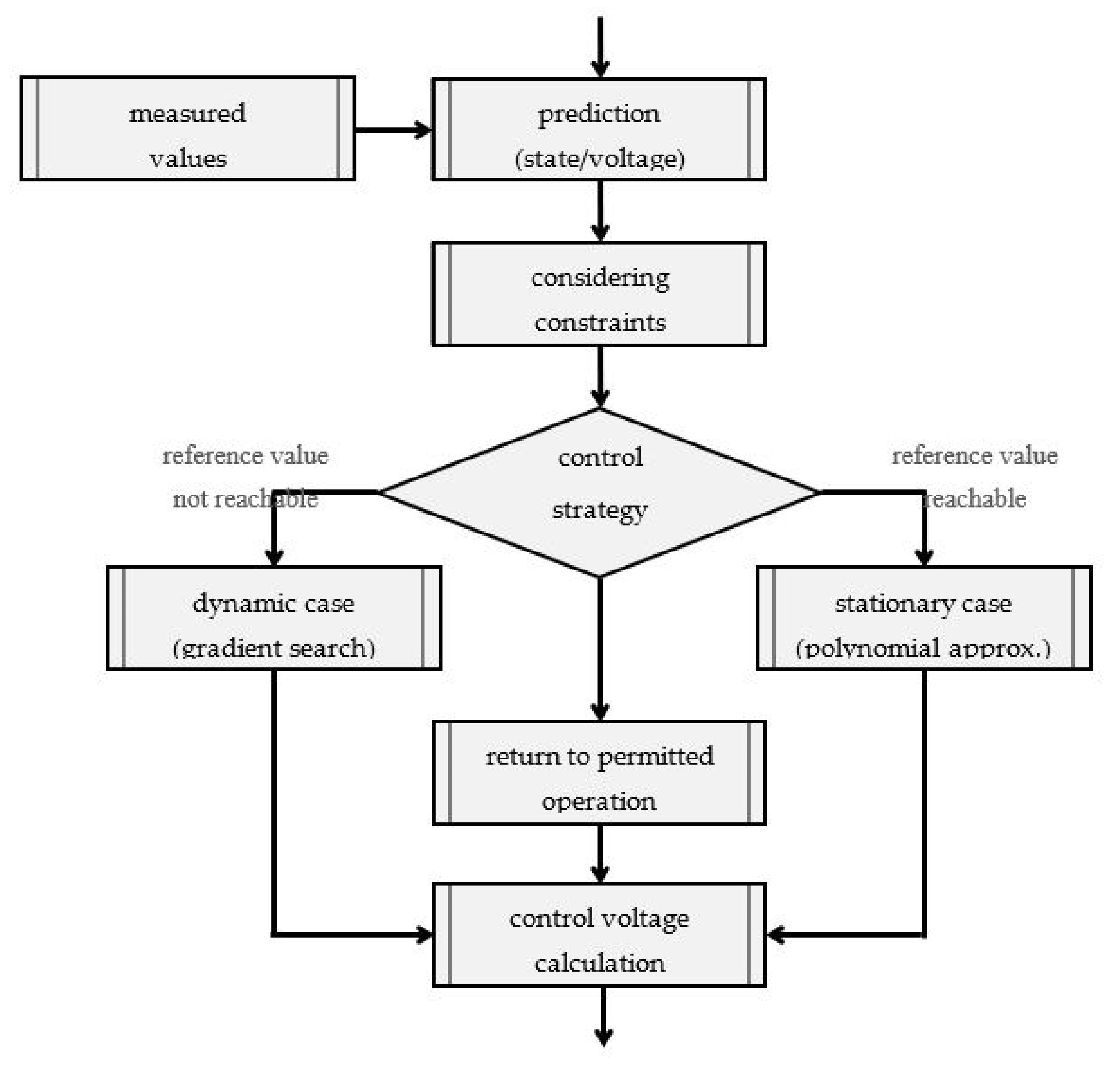
3.3. Online Torque Reference Calculation and Control

The control algorithm is visualized in Figure 6. The prediction is similar to [9] and motivated before. The control strategy is thereby divided in two main cases as follows: (1) The dynamic operation which means that the reference torque is not reachable with the given constraints due to control voltage limited hexagonal area, and (2) the stationary operation, which means that the reference torque is reachable in the next control period and inside of the constrained voltage region. If one of these cases not feasible or if it is not a plausible case, a simplified linear approach to ensure stable operation is used, but this will not be covered in this paper.

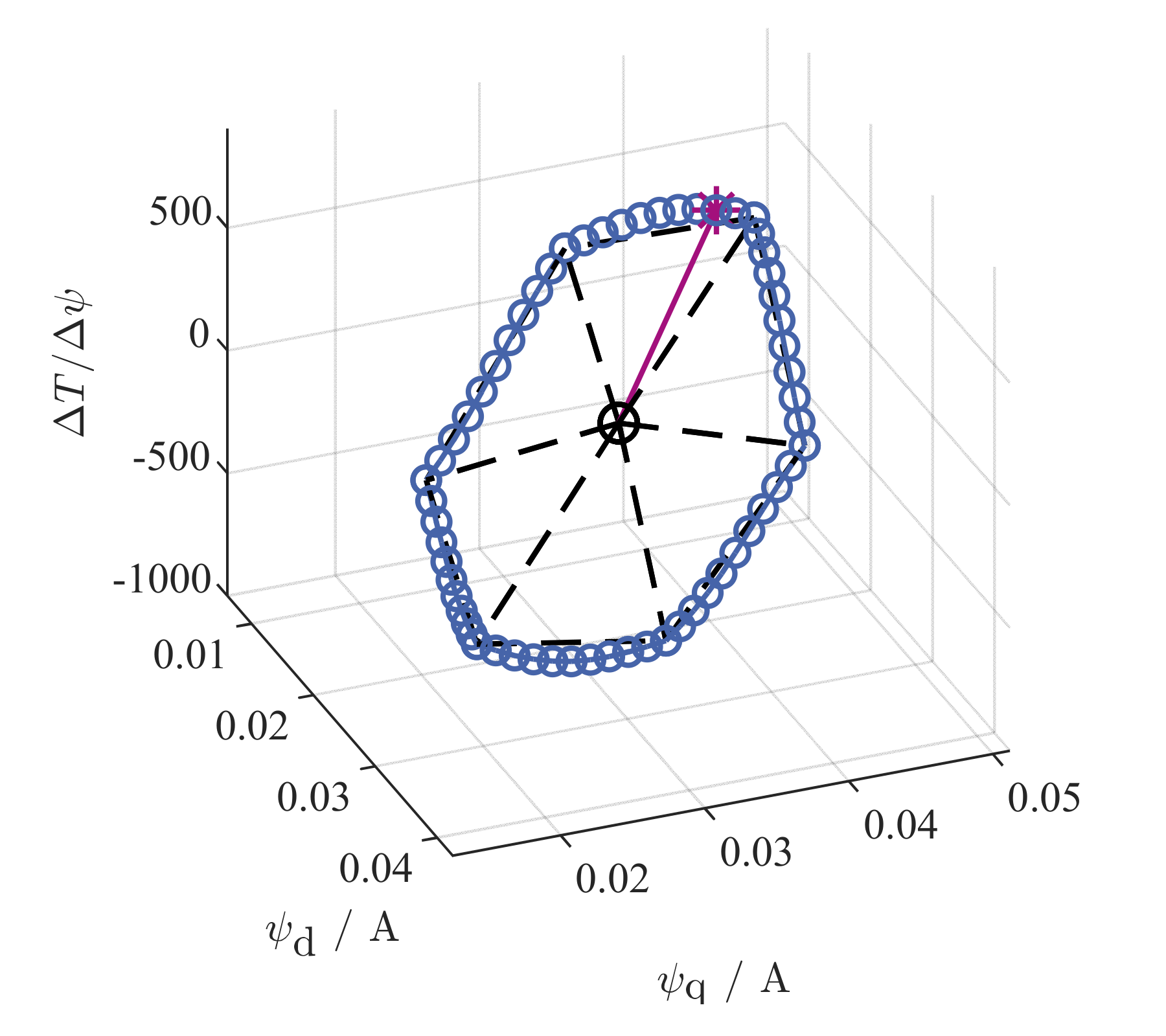
3.3.1. Dynamic Operation

The dynamic trajectory determination is implemented by an extended additional plane, the torque plane as shown in Figure 7. It is obtained by evaluating the torque according to (5) at the predicted operating points, which are determined by the flux linkages and currents. Figure 7 shows the offline calculated torque gradient of the torque plane.
To determine the online reference trajectory, we introduce a modified gradient within the torque plane. For dynamics, the gradient is acquired by calculating the difference quotient of the torque normalized on the flux-linkage plane. First, for each corner of the hexagon the torque difference to the actual torque is calculated as Δ T j , t n + 1   =   T j , t n + 1   T t n . The gradient of each corner towards the hexagon can finally be defined as   k   =   Δ T j , t n + 1 Δ ψ j , t n + 1 , with Δ ψ j , t n + 1   =   ψ d , j , t n + 1 ψ d , j , t n 2   +   ψ q , j , t n + 1 ψ q , j , t n 2 . For a more precise control, k is calculated at several supporting points between the corners via linearization. Choosing the maximum gradient with respect to the reference torque yields the target trajectory. This is visualized in Figure 8. The supporting points in this case are the d- and q-axis flux-linkages at certain rotor position and speed values. Figure 9 shows the dynamic case with the torque plane and different supporting points.

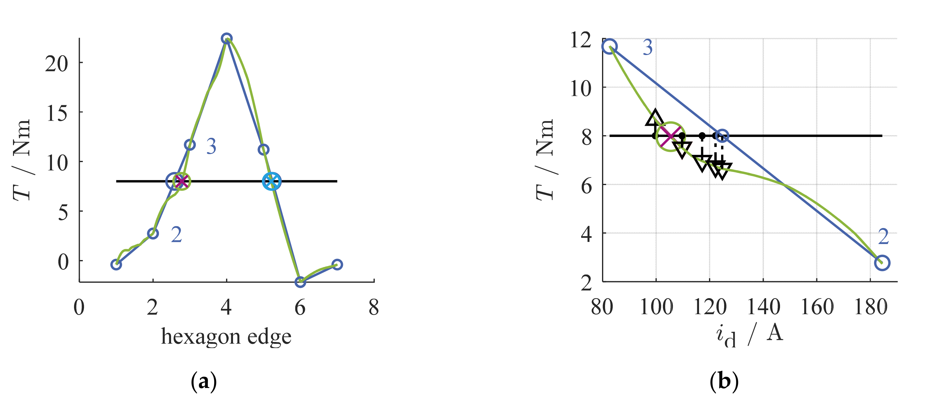
3.3.2. Stationary Operation

At stationary operation, the algorithm has to find the ideal references with maximized torque at minimal current (MTPA) or at the available voltages (MTPV). In this implementation, an iterative, real time capable procedure is implemented. Therefore, the reference iso-torque curve is approximated using a second order polynomial function of the currents looking for the maximum torque at minimum currents. At first, similar to the dynamic case, the reachable torque due to the voltage limitation is calculated. To achieve a polynomial interpolation, three supporting points are needed. Two points can be determined by linear interpolation of the torque along the edges of the prediction hexagon (the supporting points are marked in light blue and green in Figure 10). Due to nonlinearity of the torque plane the torque at the determined supporting points does not match the reference torque. Therefore, an iterative procedure is applied to achieve a convergence of the supporting points towards the reference torque. Figure 11 shows the procedure which calculates the desired value. An additional supporting point between both (marked in orange in Figure 12) allows the forming of the polynomial equation.
For the polynomial approximation, the current is assumed as i q = a i d 2 + b i d + c . Considering the three supporting points yields Equation (19). The current amplitude is defined as i abs 2 = i d 2   +   i q 2 .
i d , # 1 2 i d , # 2 2 i d , # 3 2 i d , # 1 i d , # 2 i d , # 3 1 1 1 · a b c = i q , # 1 i q , # 2 i q , # 3 ,
With (19) and the maximum current definition the polynomial function can be calculated, and the minima of the current can derived, as shown in (20).
d i d 2   +   i q 2 d i d   =   4 a 2 i d 3   +   6 a b i d 2   +   2 2 a c   +   b 2   +   1   +   2 a c   =   0 ,
The visualization of the procedure is shown in Figure 12. The determined polynomial function with the supporting points is shown in Figure 12a. The solution of the minimization is marked as star. The minimization problem for the calculation of the minimum d- und q-current is shown in Figure 12b, with the calculated minimum marked as star.
Since a second order polynomial function cannot globally approximate the iso-torque curves, iteration is performed in the direction of the previously determined MTPA point of Figure 12 (purple star) to calculate the next reference closer to the ideal reference value (both marked with purple stars) in Figure 13. If the torque difference to reference torque drops below a threshold, the iteration is completed, and the control voltage is calculated and realized. For visualization, there are two iterations drafted in the torque plane in Figure 13. Thereby the approximated curve whose supporting points lie on the hexagon’s edge and corner is the first iteration. The other curve shown is the second iteration with its respective supporting points. The solution of both iterations is marked as explained with purple stars in the figure.

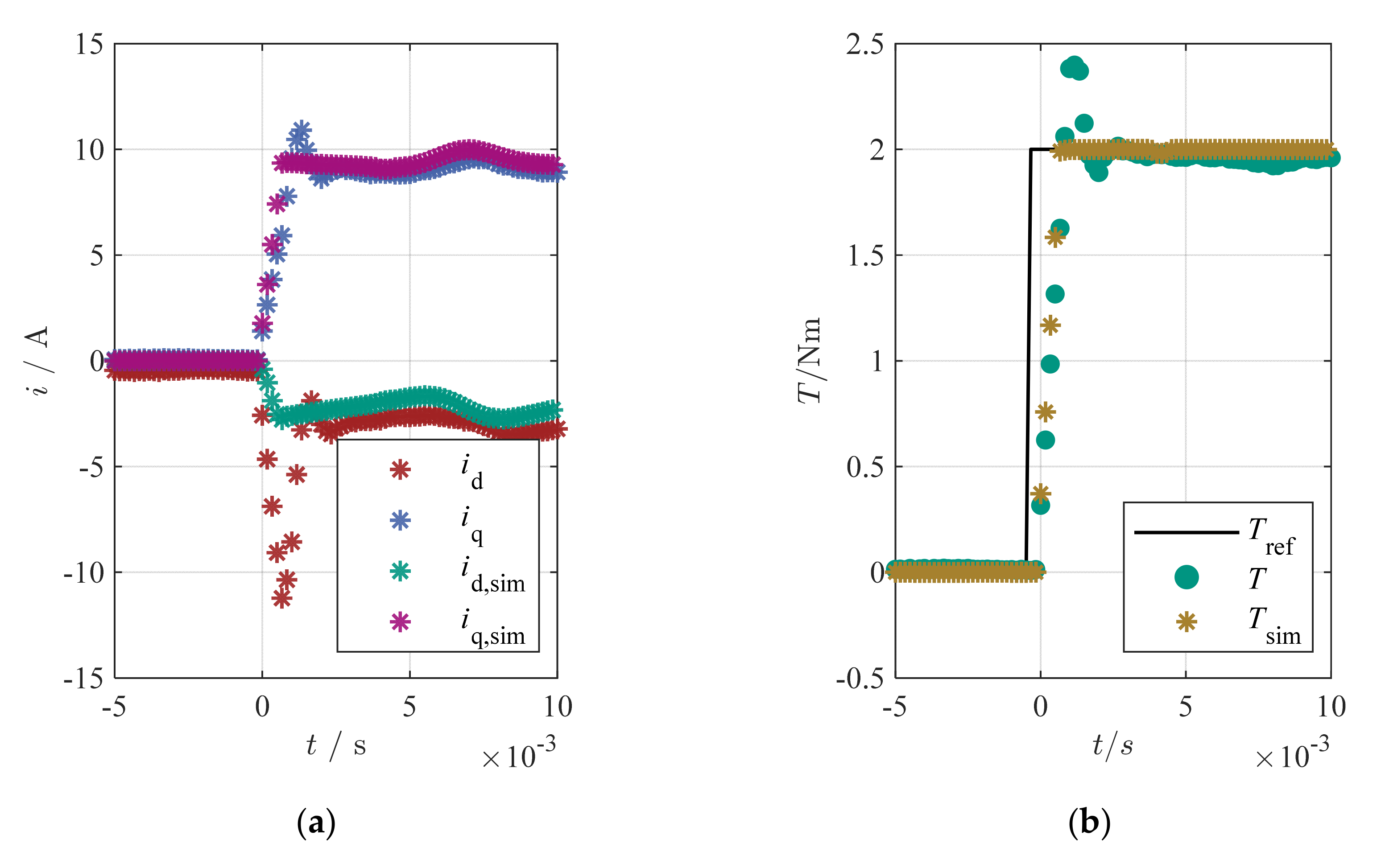
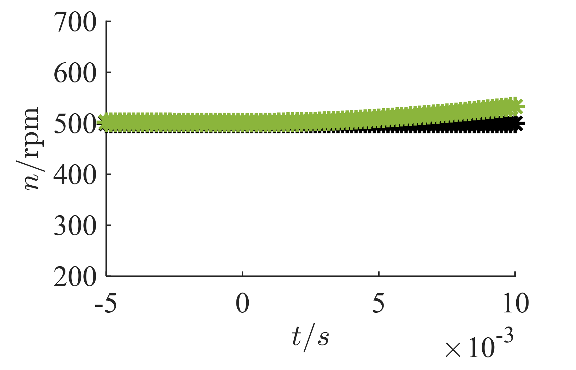
3.4. Simulation Results
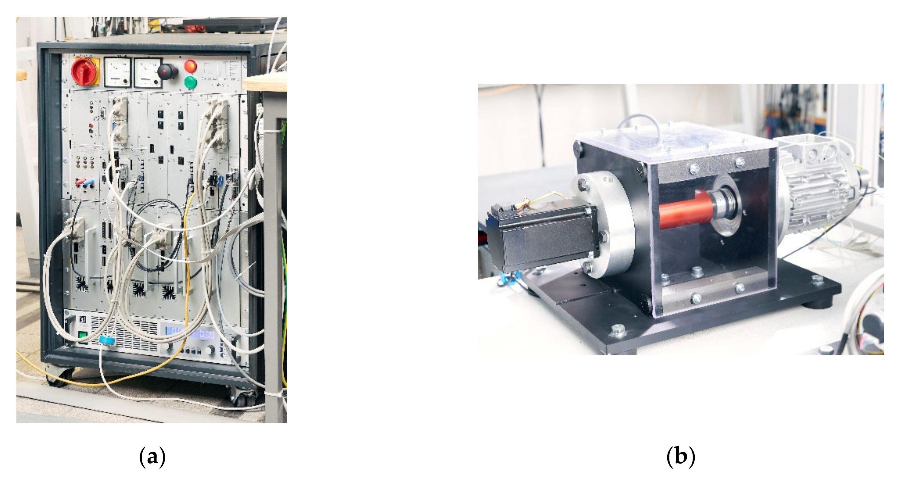
For development, the algorithm was excessively investigated in the motivated simulation environment. A simulation time-series with the dynamic and the stationary case as well as the operation within the field weakening is exemplarily shown in the following. The DC-voltage of the system was set to 250   V , the switching frequency 8   kHz . As displayed in Figure 14 the speed was set to up 500   rpm in the beginning and increased after 0.02   s to 7000   rpm for the operation at field-weakening.
The control and simulation start with no-load torque at T 0 = 0   Nm . The reference torque in the beginning is 30   Nm . At the field-weakening operation the torque must be reduced due to the limited control voltage. Therefore, the torque was also reduced to 15   Nm at 0.0225   s . In Figure 15 the resulting torque T is shown in black, the torque for control with equivalent constant currents T rip . is shown in light brown. At 0   s the control is enabled, and the dynamic case is calculated for time steps to around 0.001   s . After the dynamic control, stationary operation is enabled compensating the resulting torque harmonics. At 0.0225   s , the speed and the reference torque are changed, requiring field-weakening. At this operation, the control cannot fully compensate the torque harmonics. The calculation of the control voltage depends in this case on the present reachable area of the voltage hexagon which yields, because of the turning rotor, a time-varying area which also contains parameter mismatches due to the taken assumptions. As a result, it is only possible to damp the torque ripple not to fully mitigate it, as described and shown before.
The calculated current references can also be depicted in the d- and q-current figure as drafted in Figure 16. The red indicated points describe the operation at 30   Nm and 500   rpm . The orange is the transient operation at changing speed. The blue points are at 15   Nm and 7000   rpm . The red dots show the dynamic operation at which the algorithm follows the torque gradient as described in Section 3.3.1. The red crosses are at stationary operation with the introduced polynomial function and the minimization of the current within the voltage hexagon. The orange crosses are the reference at changing speed and torque as motivated in Figure 14 and Figure 15. The blue dot and crosses are the dynamic and stationary operation. Both the red and blue stationary operation ensure with the varying current references the compensation of the inner torque ripple.
In Figure 17 a simulative comparison, of the introduced algorithm with typical pre-calculated MTPA reference values and a predictive current control is displayed. The simulation was done at a rotor speed of 600 rpm.
For simulation, the FEA data-set considering the harmonics was utilized. The reference d- and q-currents were pre-calculated based on the corresponding fundamental flux-linkages considering the MTPA criterion. For control of these currents a predictive current control algorithm, as described in [9] is used. The parameterization of the control was done with the same fundamental flux-linkages. The controlled currents for the different torques are shown in Figure 17b. The corresponding torque is shown in Figure 17a as expected the torque is not constant due to the flux-linkage harmonics. In contrast in Figure 17c shows the smooth torque (in brown), controlled with the introduced algorithm and also the torque of the presented method in Figure 17a. In Figure 17d the online calculated reference currents are displayed. It is visible that these currents match the pre-calculated currents. The additional ripple of these currents is due to the minimization of the inner torque ripple as described before.

4. Test-Setup

The introduced algorithm is implemented as described in simulation and on a test-bench. The used hardware and software for the testing and validation is following shown.

4.1. Device-Under-Test

As device under test, a special manually manufactured PMSM prototype based on a commercial stator and rotor lamination from Kienle + Spiess of the type KSPM 80/4.70 was available for the testbench measurements. The device under test is built up with distributed windings and is, in this case, star connected. The main quantities are displayed in Table 1.
The measured flux-linkages for a constant speed and a fixed rotor position are shown in Figure 18a,b. These flux linkages are used for the test-bench implementation and the following measurement results. As described before for the development of the algorithm and the visualization FEA generated data are used.

4.2. Test-Bench Setup

The back to back mounting of the device under test and the load machine is shown in Figure 19b. The device under test (right side) and the load machine (left side). The load machine is a PMSM type Nanotec DB80C04803-ENM05J. The used voltage source inverters have a shared DC-link, supplied by a DC power supply. The inverter MOSFETs are of the type Texas Instrument CSD19535KCS with a switching frequency of 6   kHz . The currents for the control of the DUT are measured by current transducers of type LEM LAX 100-np. The voltages are directly measured via precise voltage dividers. The sampling frequency of the ADCs, type Texas Instrument THS 1206 (12 bit), is 1.5 Msps. The rotor speed and the rotor position are determined with a Heidenhain ROC1013 13-bit encoder. The load machine is speed controlled by a standard cascaded PI type control algorithm. The control is done by a TMS320C6748 digital signal processor from Texas Instruments. The introduced control algorithm for the device under test, runs on an ARM Cortex A-9 in a Xilinx System-on-Chip device of type Zynq-Z7030 in real-time. The control period is T c   =   166.6   μ s , according to the switching frequency of 6   kHz . The inverter switching signals are generated on a Cyclone IV field programmable gate array from Intel. A more detailed view of the modular signal processing system can be found in [18] and [19]. The whole power electronics and signal processing system cabinet is shown in Figure 19a.

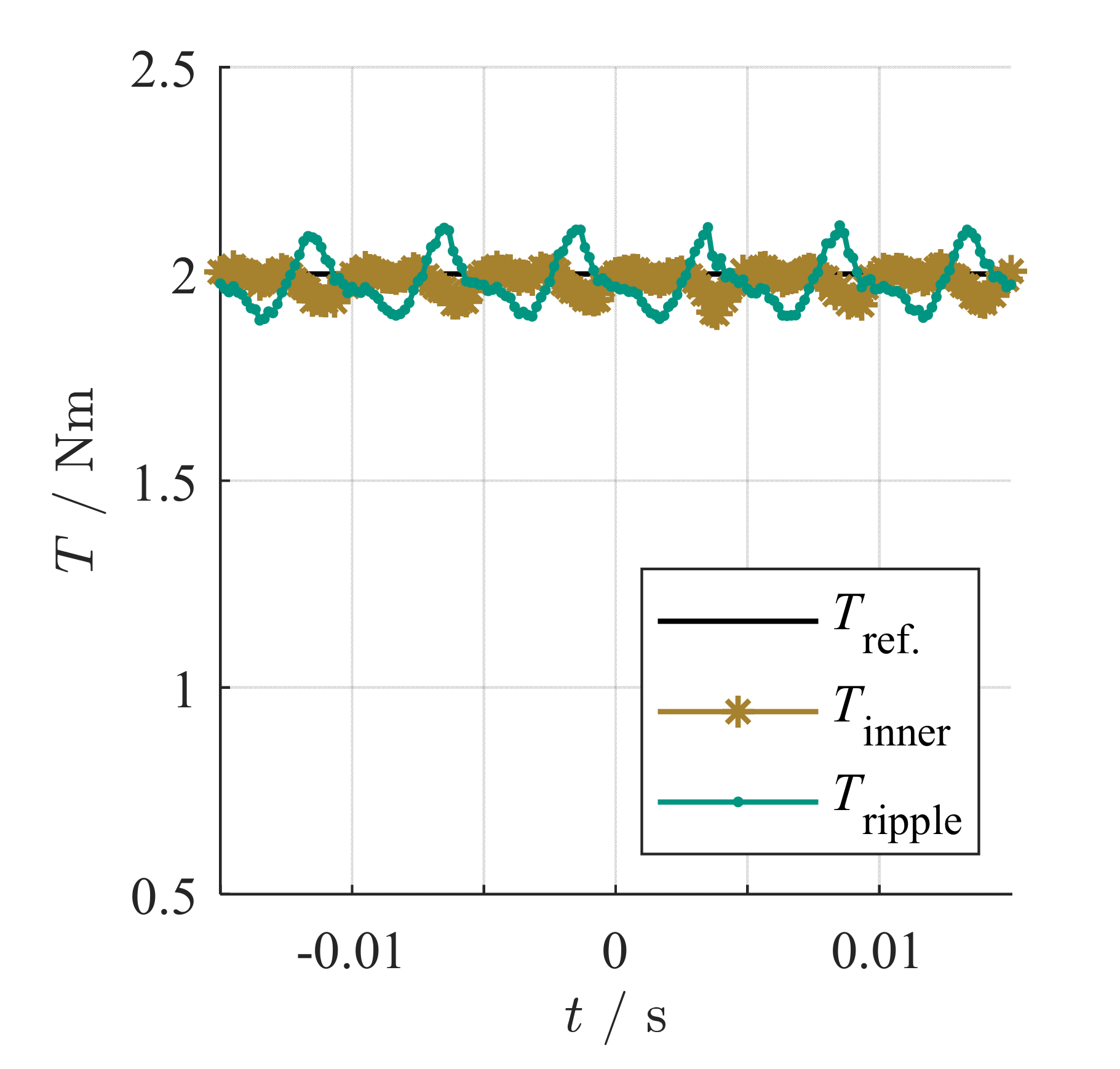
5. Measurement Results

In this section the measurement and implementation results of the test-bench realization, as a complementation to the derived theory and simulated control algorithm, are shown. This section focuses on the proof of concept of the algorithm and especially the real-time-capability. For verification, a comparative measurement with simulation and the same parameters of both, is shown. Intensive investigations of the stationary and dynamic control behavior in the whole operating range are not subject in this paper but are subject to future work. The measurements are done with the available device under test on the introduced test-bench, the flux-linkages of the PMSM are shown in Figure 18. The stator resistance is identified to 340   m Ω .

Test-Bench Measurement

As described in the test-bench section, the algorithm is implemented on the introduced signal processing hardware based on a Zynq-Z7030. The necessary lookup-tables ( i dq ψ d , ψ q , γ and ψ dq i d , i q , γ ) are stored in the DDR memory of the device. The control algorithm itself is real-time capable with a calculation time of 90   μ s at the dynamic case and 105   μ s for the stationary operation, including the peripheral control and management of the test-bench. The inverter switching frequency is set to 6   kHz . The shown torque is the inner torque, calculated based on the flux-linkages. Even with the torque meter, the measured torque would be unreliable, because of the not separable load machine torque ripple, the damping of the clutches, the shaft, the torque meter, and other parasitic effects. For precise torque measurement without calculations a special test-bench could be necessary.
Figure 20 shows a torque step from zero torque to 2   Nm . The speed is controlled by the load machine to 500   rpm . The brown line is the inner torque according to Equation (5). The brown stars describe the beginning of each discrete control period T c . . The reference torque is reached with the gradient search within seven control periods T c . This can also be seen in Figure 21. The values from bottom right to the left show the gradient search algorithm in the torque plane as introduced in Figure 7. After an intersection with the reference iso-torque curve has been detected, the stationary case is applied. This is achieved by approximation of the iso-torque curve and searching for the minimum current at this curve. The heap of the values shows both, the reference flux-linkage and the current reference values which yield a smooth inner torque of the PMSM. The green dotted curve in Figure 20 displays an equivalent operational point with constant currents without compensation of the inner torque ripple. Considering the position depended flux-linkages for the control, as shown by the brown line, yields in a smoother torque. With the inner torque ripple compensation parasitic effects, measurement inaccuracies, nonlinearities, mismatch of the used parameters, and other effects still influence the controlled torque and show differences compared to the simulations which shows ideal smooth inner torque. However, compared to control with constant currents, the torque ripple is significantly reduced.
Figure 22 shows the stationary operation close to the nominal speed. The brown controlled torque is the controlled inner torque with the new approach, the green curve with the ripple controlled at equivalent constant currents. The displayed results show the feasibility and effectiveness of the approach even with the requirements for real-time capability and testbench operation.
In Figure 23 an additional comparison of simulation and measurement is shown as confirmation of the simulation environment, simulation results and test-bench measurements. In Figure 23a, the simulated and measured currents are displayed. The simulation currents are blue and red, the measured currents are green and purple. The rise time thereby is almost the same. The overshot of the measured currents can be explained with the difference in the rotor speed as shown in Figure 24.
Due to the fast torque step the load machine’s standard PI speed controller is not able to ensure constant speed in this short time. Moreover, parameter mismatches, in particular for the simple model of the used inverter and the wiring could be not sufficient. However, the changing currents, clearly show the same behavior in simulation as well as in the measurement for the minimization of the inner torque ripple. In Figure 23b, the corresponding torque is shown where simulation in green look similar to the results in brown. The marked discrete sampling points of both, are looking also good even the absolute timings differ, which is because the not ideal superposition of simulation and measurement results.

6. Discussion and Conclusions

This paper shows an approach for predictive trajectory control with online MTPA calculation and minimization of the inner torque ripple of PMSMs.

6.1. Parameteridentification and Modelling

The basic machine equations and assumptions, particularly the extended torque equation, are motivated in the beginning of this paper. For the developed control algorithm which considers the inner torque ripple of the PMSM, the position dependent flux-linkages are mandatory.
The theory and principle for the challenging test-bench identification of these position dependent flux-linkages, using Fourier analysis and solving the differential equation, is shown. Based on the identified model parameters of the flux-linkages and the stator resistance an acausal simulation environment is parameterized. This simulation environment enables rapid control prototyping and provides the shown simulation results and explanations of the derived control algorithm.
The extension of a predictive trajectory control algorithm, adapted by the current plane, the flux-linkage plane and the voltage-plane with the machines inner torque yields not only the possibility for the online calculation of the reference torque values, including the position-dependent flux-linkages yields also the possibility of the inner torque ripple compensation.

6.2. Introduced Control Algorithm

The introduced control algorithm is split up in two main cases. (1) The dynamic operation which executes an online gradient search on the introduced torque plane for the fast response to the reference torque as described in Section 3.3.1. (2) The stationary operation (Section 3.3.2) has the goal of a minimal current for a maximum torque under certain restrictions as the available voltage of the inverter, the current limitation, and the present state of the machine. At stationary operation, the online-capable iterative polynomial approximation of the iso-torque curve solves the minimization problem for ideal reference values. Considering these cases and constraints in the algorithm enables the control with online MTPA calculation and the compensation of the inner torque ripple.

6.3. Results

In this paper the control algorithm is explained in detail, supported with realistic parameter based simulations for understanding. Both, the dynamic case, and stationary case are shown with corresponding simulations. The verification of the simulation results and the test-bench measurements is done by a comparison of both. Furthermore, the testbench implementations and the measurements shows that the algorithm is fully real-time-capable at 6 kHz control frequency without further optimizations. The testbench results also indicate an improvement of the controlled torque compared to state-of-the-art control with constant and precalculated MTPA/MTPV currents. Furthermore, with the introduced approach no additional lookup table necessary for the torque to current references as used in classical offline calculated MTPA strategies. The online calculated torque to current references offer new possibilities as parameter adaption by online identification or thermal observers without the need to manipulate the MTPA/MTPV reference parameters during control. The measurements and the test-bench implementations show the efficiency of the introduced algorithm. However, for global statements, further investigations are necessary. Investigations of the precise and detailed control behavior in the whole operating range, stability analysis, and measurement with special test-benches which allow precise torque ripple measurement, has to be done in further research and will probably published in future papers.

Author Contributions

Conceptualization, S.D., M.B. (Matthias Brodatzki) and B.B.; methodology, S.D. and M.B. (Matthias Brodatzki); software, S.D., B.B. and B.S.-R.; validation, S.D., B.S.-R. and B.B.; formal analysis, S.D., M.B. (Matthias Brodatzki) and B.B; writing—original draft preparation, S.D.; writing—review and editing, M.B. (Matthias Brodatzki), B.B., B.S.-R. and A.L.; visualization, S.D. and B.B.; supervision, M.H., A.L. and M.B. (Michael Braun). All authors have read and agreed to the published version of the manuscript.

Funding

This research received no external funding.

Acknowledgments

We acknowledge support by the KIT-Publication Fund of the Karlsruhe Institute of Technology. The author would thank also to his former tutor and working colleague Jan Richter for the ideas and preliminary work at the institute of electrical engineering in Karlsruhe.

Conflicts of Interest

The authors declare no conflict of interest.

References

  1. Han, Z.; Liu, J.; Yang, W.; Pinhal, D.B.; Reiland, N.; Gerling, D. Improved Online Maximum-Torque-Per-Ampere Algorithm for Speed Controlled Interior Permanent Magnet Synchronous Machine. IEEE Trans. Ind. Electron. 2020, 67, 3398–3408. [Google Scholar] [CrossRef]
  2. Tinazzi, F.; Bolognani, S.; Calligaro, S.; Kumar, P.; Petrella, R.; Zigliotto, M. Classification and review of MTPA algorithms for synchronous reluctance and interior permanent magnet motor drives. In Proceedings of the 2019 21st European Conference on Power Electronics and Applications (EPE ’19 ECCE Europe), Genova, Italy, 3–5 September 2019; pp. 1–10. [Google Scholar]
  3. Wang, J.; Huang, X.; Yu, D.; Chen, Y.; Zhang, Y.; Niu, F.; Fang, Y.; Cao, W.; Zhang, H. An Accurate Virtual Signal Injection Control of MTPA for an IPMSM With Fast Dynamic Response. IEEE Trans. Power Electron. 2018, 33, 7916–7926. [Google Scholar] [CrossRef] [Green Version]
  4. Lee, G.-H.; Kim, S.-I.; Hong, J.-P.; Bahn, J.-H. Torque Ripple Reduction of Interior Permanent Magnet Synchronous Motor Using Harmonic Injected Current. IEEE Trans. Magn. 2008, 44, 1582–1585. [Google Scholar] [CrossRef]
  5. Nishio, T.; Ryosuke, Y.; Masahiko, K.; Akatsu, K. A Method of Torque Ripple Reduction by Using Harmonic Current Injection in PMSM. In Proceedings of the 2019 IEEE 4th International Future Energy Electronics Conference (IFEEC), Singapore, 25–28 November 2019; pp. 1–5. [Google Scholar]
  6. Li, S.; Han, D.; Sarlioglu, B. Modeling of Interior Permanent Magnet Machine Considering Saturation, Cross Coupling, Spatial Harmonics, and Temperature Effects. IEEE Trans. Transp. Electrific. 2017, 3, 682–693. [Google Scholar] [CrossRef]
  7. Cho, H.-J.; Kwon, Y.-C.; Sul, S.-K. Optimal Current Trajectory Control of IPMSM for Minimized Torque Ripple. In Proceedings of the 2019 IEEE Transportation Electrification Conference and Expo (ITEC), Detroit, MI, USA, 19–21 June 2019; pp. 1–6. [Google Scholar]
  8. Farshadnia, M.; Cheema, M.A.M.; Dutta, R.; Fletcher, J.E.; Rahman, M.F. Detailed Analytical Modeling of Fractional-Slot Concentrated-Wound Interior Permanent Magnet Machines for Prediction of Torque Ripple. IEEE Trans. Ind. Applicat. 2017, 53, 5272–5283. [Google Scholar] [CrossRef]
  9. Richter, J.; Doppelbauer, M. Predictive Trajectory Control of Permanent-Magnet Synchronous Machines with Nonlinear Magnetics. IEEE Trans. Ind. Electron. 2016, 63, 3915–3924. [Google Scholar] [CrossRef]
  10. Krause, P.C.; Wasynczuk, O.; Sudhoff, S.D. Analysis of Electric Machinery and Drive Systems; Wiley-Interscience: Hoboken, NJ, USA; IEEE Press: New York, NY, USA, 2002. [Google Scholar]
  11. Pinto, D.E.; Pop, A.-C.; Kempkes, J.; Gyselinck, J. Dq0-modeling of interior permanent-magnet synchronous machines for high-fidelity model order reduction. In Proceedings of the 2017 International Conference on Optimization of Electrical and Electronic Equipment (OPTIM) & 2017 Intl Aegean Conference on Electrical Machines and Power Electronics (ACEMP), Brasov, Romania, 25–27 May 2017; pp. 357–363. [Google Scholar]
  12. Štumberge0r, G.; Štumberger, B.; Marčič, T. Magnetically Nonlinear Dynamic Models of Synchronous Machines and Experimental Methods for Determining their Parameters. Energies 2019, 12, 3519. [Google Scholar] [CrossRef] [Green Version]
  13. Richter, J.; Doppelbauer, M. Control and mitigation of current harmonics in inverter-fed permanent magnet synchronous machines with non-linear magnetics. IET Power Electron. 2016, 9, 2019–2026. [Google Scholar] [CrossRef]
  14. Decker, S.; Rollbühler, C.; Rehm, F.; Brodatzki, M.; Oerder, A.; Liske, A.; Kolb, J.; Braun, M. Dq0-modelling and parametrization approaches for small delta connected permanent magnet synchronous machines. In Proceedings of the 2020 International Conference on Power Electronics, Machines and Drives (PEMD 2020), Nottingham, UK, 15–17 December 2020. [Google Scholar]
  15. Decker, S.; Foitzik, S.; Rehm, F.; Brodatzki, M.; Rollbühler, C.; Kolb, J.; Braun, M. DQ0 Modelling and Parameterization of small Delta connected PM Synchronous Machines. In Proceedings of the 2020 International Conference on Electrical Machines (ICEM), Göteborg, Sweden, 23–26 August 2020. [Google Scholar]
  16. Richter, J.; Dollinger, A.; Doppelbauer, M. Iron loss and parameter measurement of permanent magnet synchronous machines. In Proceedings of the 2014 International Conference on Electrical Machines (ICEM), Berlin, Germany, 2–5 September 2014; pp. 1635–1641. [Google Scholar]
  17. Richter, J.; Winzer, P.; Doppelbauer, M. Einsatz Virtueller Prototypen bei der Akausalen Modellierung und Simulation von Permanenterregten Synchronmaschinen. Application of Virtual Prototypes of Permanent Magnet Synchronous Machines by Acausal Modeling and Simulation; VDE-Verlag: Berlin, Germany, 2013. [Google Scholar]
  18. Axtmann, C.; Boxriker, M.; Braun, M. A custom, high-performance real time measurement and control system for arbitrary power electronic systems in academic research and education. In Proceedings of the 2016 18th European Conference on Power Electronics and Applications (EPE’16 ECCE Europe), Karlsruhe, Germany, 5–9 September 2016; pp. 1–7. [Google Scholar]
  19. Schwendemann, R.; Decker, S.; Hiller, M.; Braun, M. A Modular Converter- and Signal-Processing-Platform for Academic Research in the Field of Power Electronics. In Proceedings of the 2018 International Power Electronics Conference (IPEC-Niigata 2018 -ECCE Asia), Niigata, Japan, 20–24 May 2018; pp. 3074–3080. [Google Scholar]
Figure 1. Result of the reference torque calculation. The x-axis denotes the direct current, the y-axis the quadrature current. The torque hyperbolas (iso-torque curves) in grey are calculated considering the machines flux-linkages and currents. The maximum current magnitude is the red dotted circle. The maximum torque per ampere (MTPA) locus for maximum torque at minimum current is the solid red line. The maximum torque per volt/voltage (MTPV) locus for maximum torque at constrained voltage is the solid blue line.
Energies 13 05327 g001
Figure 2. Equivalent circuit model: (a) of the d-axis component; (b) of the q-axis component.
Energies 13 05327 g002
Figure 3. Finite element analysis (FEA)-calculated flux-linkages for the used machine in simulation and for the explanations, assuming   ω = const . at a fixed rotor position   γ : (a) flux-linkage of the direct-axis (b) flux-linkage of the quadrature-axis. The displayed data are of a machine with a maximum speed up to   15.000   rpm at   70   kW peak power at a voltage of   300   V DC .
Energies 13 05327 g003
Figure 4. Different planes: (a) current plane; (b) flux-linkage plane; (c) voltage plane. The planes (a), (b), and (c) are showing the latest operating point (small black circle). The reachable operating points inside the blue hexagon and chosen trajectory considering of each time-step and voltage hexagon (purple star). The current limitation of the machine is marked as red circle. In (c) also the rotating inverter voltage hexagon with the black inner circle is drafted.
Energies 13 05327 g004
Figure 5. Visualization of the different control periods with sampling, prediction, and reference value calculation within the control procedure.
Energies 13 05327 g005
Figure 6. Simplified diagram of the introduced control algorithm, executed for each control period.
Energies 13 05327 g006
Figure 7. Torque plane (z-axis) at present current, speed and rotor position. The gradient of the ideal reference torque trajectory is the black line, the actual torque the black circle. The boundaries are marked as blue voltage hexagon and the chosen next reference value is in purple. The reference torque is the red star with the offline calculated red MTPA trajectory for ideal steady-state operation.
Energies 13 05327 g007
Figure 8. Calculation of the ideal reference value considering the gradient   k with   Δ T Δ ψ under the certain constraints. The purple arrow shows the chosen reference value with optimal trajectory.
Energies 13 05327 g008
Figure 9. Dynamic case: (a) and (b) torque contour lines (z-axis) and constraint area due to the applicable voltage hexagon in blue, present value as black circle. In (a) the current plane (x- and y-axis) is shown, (b) shows it in the equivalent flux linkage plane. The purple arrow shows the chosen reference value from Figure 8 with fastest achievable torque for the next control period.
Energies 13 05327 g009
Figure 10. Stationary case (first iterations of two): With torque contour lines (surface) and constraint area due to the applicable voltage hexagon in blue and the current limit in red. (#1) to (#3) are the values for the polynomial approximation, (*) is the solution of the first iteration of the polynomial approximation. As visible, the first approximation of the iso-torque curve (purple) does not suit the iso-torque curve, another iteration is necessary. The x- and y-axis are the direct and quadrature currents.
Energies 13 05327 g010
Figure 11. Supporting points with intersection to the hexagonal area: Both diagrams with reference torque in black, present torque (iso-curve) in green. (a) hexagon edges with corresponding torque intersection. As shown in Figure 10 both hexagon edges (2 and 3) with the chosen supporting point (d- and q-current) marked with the purple cross and the green circle. (b) shows the selection of the desired value by considering the sign and the intersection of the reference torque with the different iterations displayed with black arrows. As a result, the desired value is identified as purple cross and the green circle similar to Figure 10.
Energies 13 05327 g011
Figure 12. Stationary case: (a) Second order polynomial approximated d- and q-current (red dashed line). The supporting points are marked with black circles, the solution of the minimization problem (b) is marked as star. (b) shows the minimization problem as described in (20).
Energies 13 05327 g012
Figure 13. Stationary case with two iterations: The area, which is attainable within the control period is enclosed by the blue hexagon. The current limit is displayed in red. The surface describes the machine torque. Both iterations of the polynomial approximation are shown in purple. The first iteration (Figure 10) does not match the iso-torque curve, where the second iteration matches well with the green iso-torque curve within the range of interest.
Energies 13 05327 g013
Figure 14. Simulation setup with 500 rpm in the beginning and increased after 0.02 s to 7000 rpm for the operation at field-weakening. In Figure 15 is the corresponding torque displayed.
Energies 13 05327 g014
Figure 15. Operation of the control algorithm at two different torques. The corresponding speed is shown in Figure 14. The torque T, controlled with the introduced algorithm, is shown in black, the torque for control with equivalent constant currents   T rip . is shown in light brown.
Energies 13 05327 g015
Figure 16. Simulation of the trajectory in red at 30 Nm and 500 rpm, with the red dots at dynamic operation and the red crosses at stationary operation. In blue at 15 Nm and 7000 rpm, with the blue dots at dynamic operation and the blue crosses at stationary operation. The orange crosses show the behavior during changing the speed.
Energies 13 05327 g016
Figure 17. Torque control with a fundamental predictive control algorithm and pre-calculated reference values in (b) the controlled currents to the corresponding torque (a) are displayed. In (c) the torque of the introduced algorithm is shown in brown. The minimized torque ripple is displayed black. (d) shows the corresponding online calculated currents including the current ripple needed for the minimization of the torque ripple. The simulations were done at 600 rpm rotor speed.
Energies 13 05327 g017
Figure 18. Measured/estimated flux-linkages of the device under test at the test-bench, assuming   ω = 1000   rpm at a fixed rotor position   γ = 60 ° : (a) flux-linkage of the direct-axis (b) flux-linkage of the quadrature-axis.
Energies 13 05327 g018
Figure 19. Test-bench setup: (a) Testbench cabinet with inverters and signal processing; (b) mechanical assembly of device under test and load machine (Source: Amadeus Bramsiepe, KIT).
Energies 13 05327 g019
Figure 20. Torque step from zero torque to   2   Nm at   500   rpm . The reference torque is thereby displayed black, the present inner torque (according Equation (5)) calculated as describe before is brown. The predicted torque used in the control is shown as purple line. The torque in this operational point, controlled with equivalent constant currents (as is done in fundamental approaches without torque ripple compensation) is shown as green dashed line.
Energies 13 05327 g020
Figure 21. Current plane (a) and flux-linkage plane (b) with the currents/flux-linkages at each time step. The values form bottom right to the left show the gradient search algorithm. After the intersection with the iso-torque curve the stationary case is applied. The heap of the values is due to the stationary torque ripple compensation.
Energies 13 05327 g021
Figure 22. Stationary operation close to the nominal speed with   1000   rpm at   2   Nm . In brown: the inner torque applied by the introduced control. In green the torque with uncompensated ripple, controlled with equivalent constant. Black shows the reference torque.
Energies 13 05327 g022
Figure 23. Measurement and equivalent simulation of (a) current response (measurement in green and purple, simulation in red and blue) and (b) torque response (measurement in brown, reference torque in black and simulation in green) at a rotor speed of 500 rpm.
Energies 13 05327 g023
Figure 24. Rotor speed of the measurement in green and constant rotor speed of 500 rpm in the simulation.
Energies 13 05327 g024
Table 1. Main quantities of the device under test.
QuantitiesSymbolValue
Maximum voltage v 48   V
Maximum current i 16   A
Nominal speed n 1000   rpm
Nominal torque T 3.3   Nm
Permanent magnet flux-linkage   ψ PM 70.1   mVs
Stator resistance R 340   m Ω
Publisher’s Note: MDPI stays neutral with regard to jurisdictional claims in published maps and institutional affiliations.

