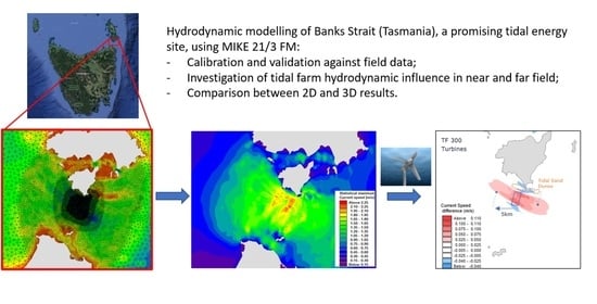
Towards a Tidal Farm in Banks Strait, Tasmania: Influence of Tidal Array on Hydrodynamics


Abstract
1. Introduction
2. Modelling Methodology
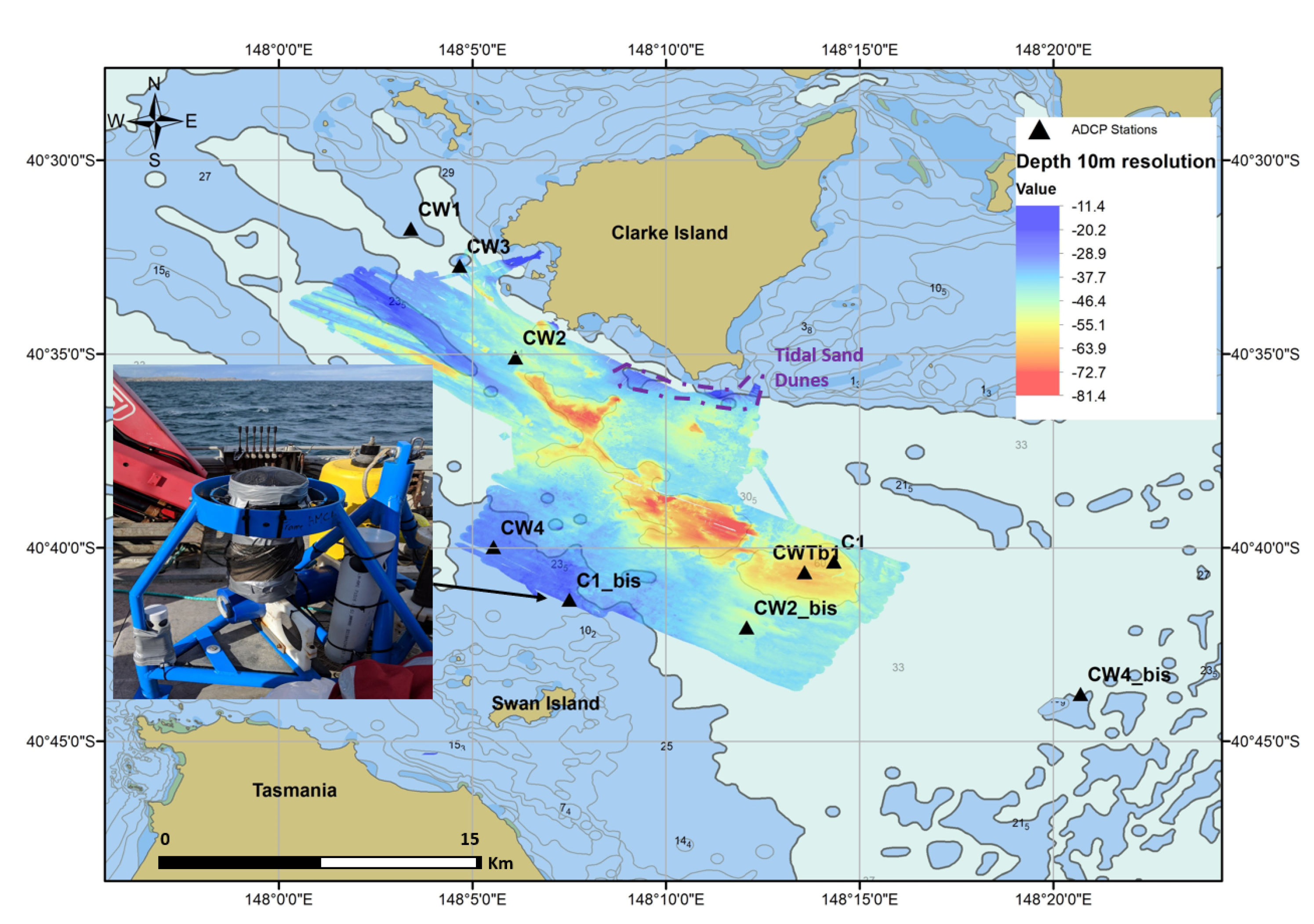
2.1. The Site and Data Collection
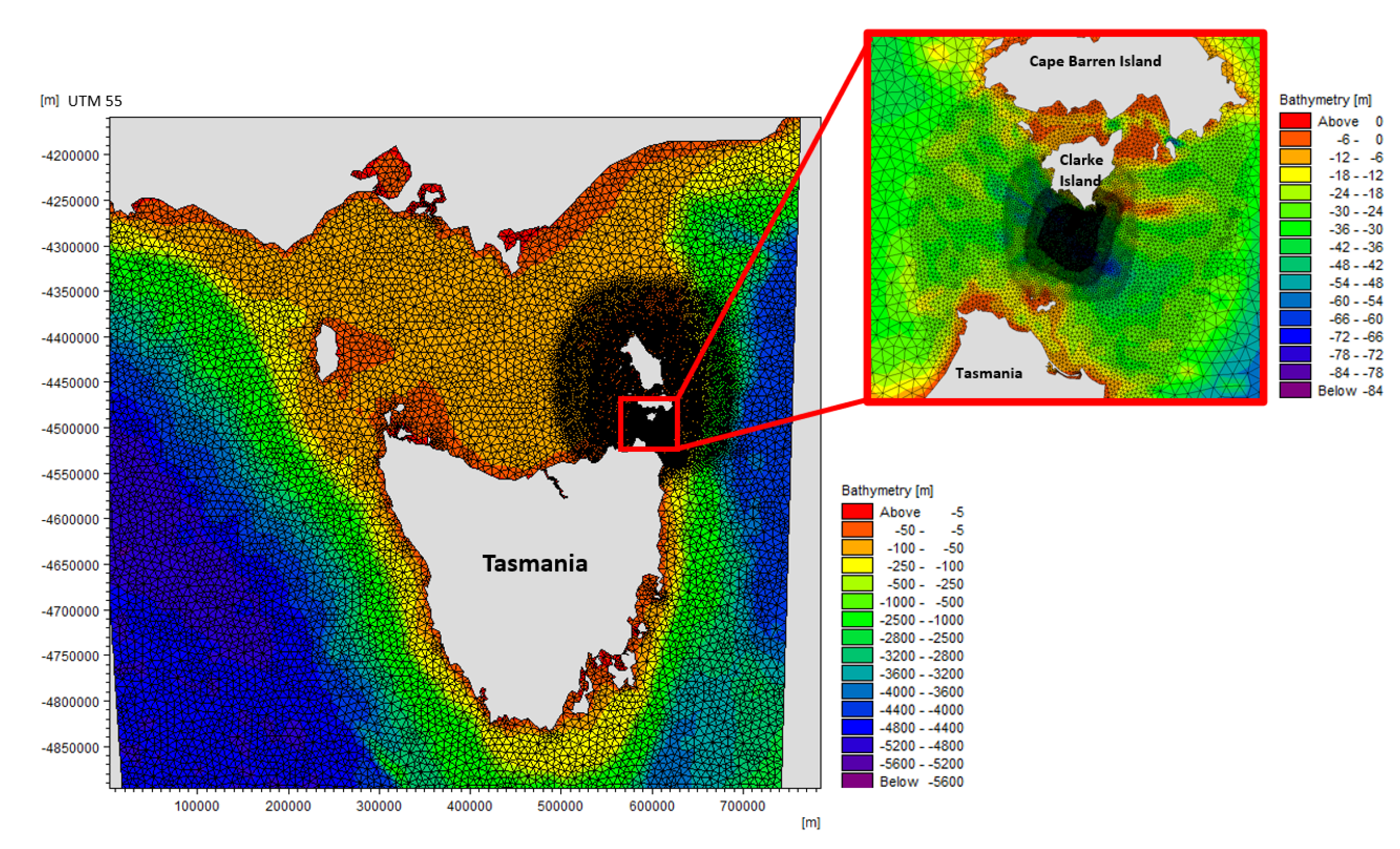
2.2. Model Domain and Forcing
2.3. Model Settings
3. Validation
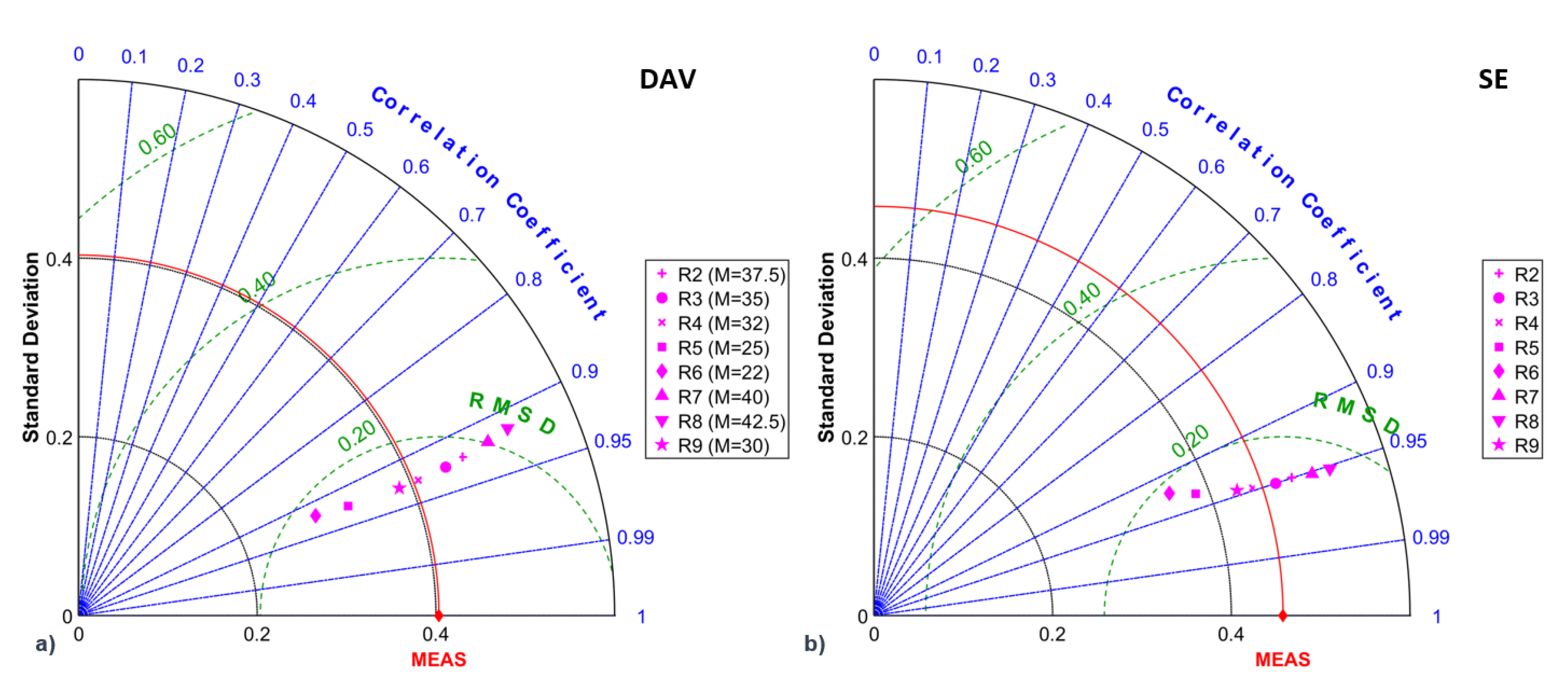
3.1. Calibration
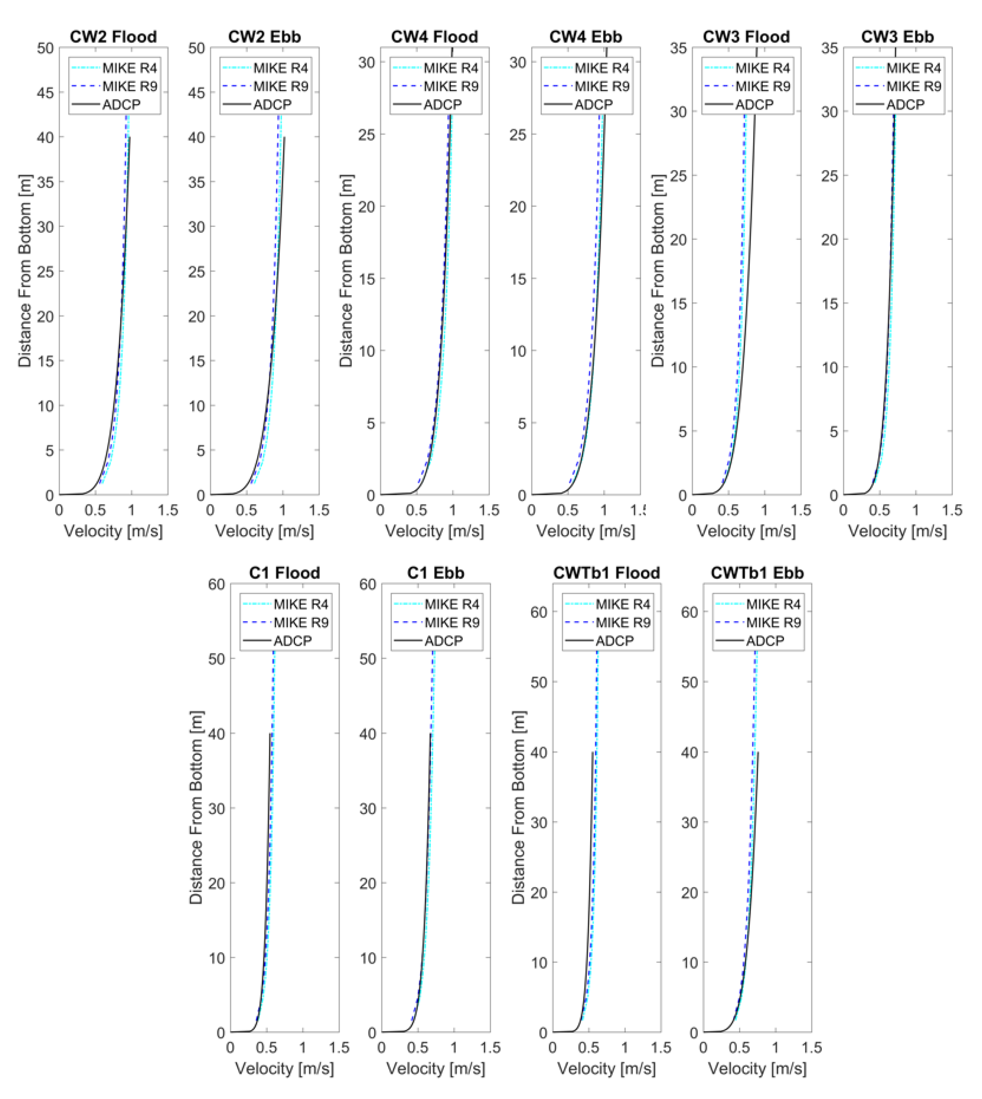
3.1.1. Free Surface and Velocities
3.1.2. Harmonic Analysis
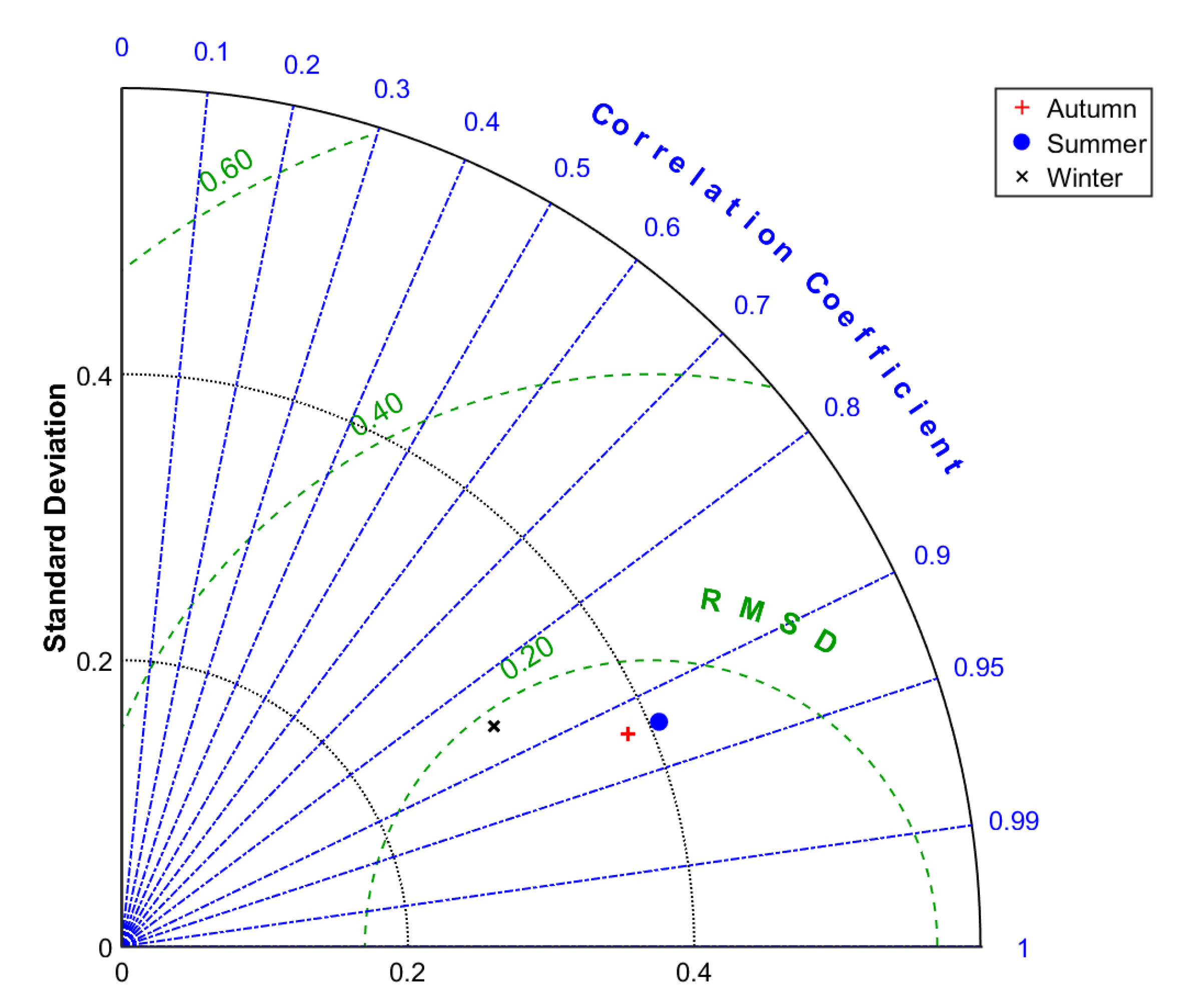
3.1.3. Validation
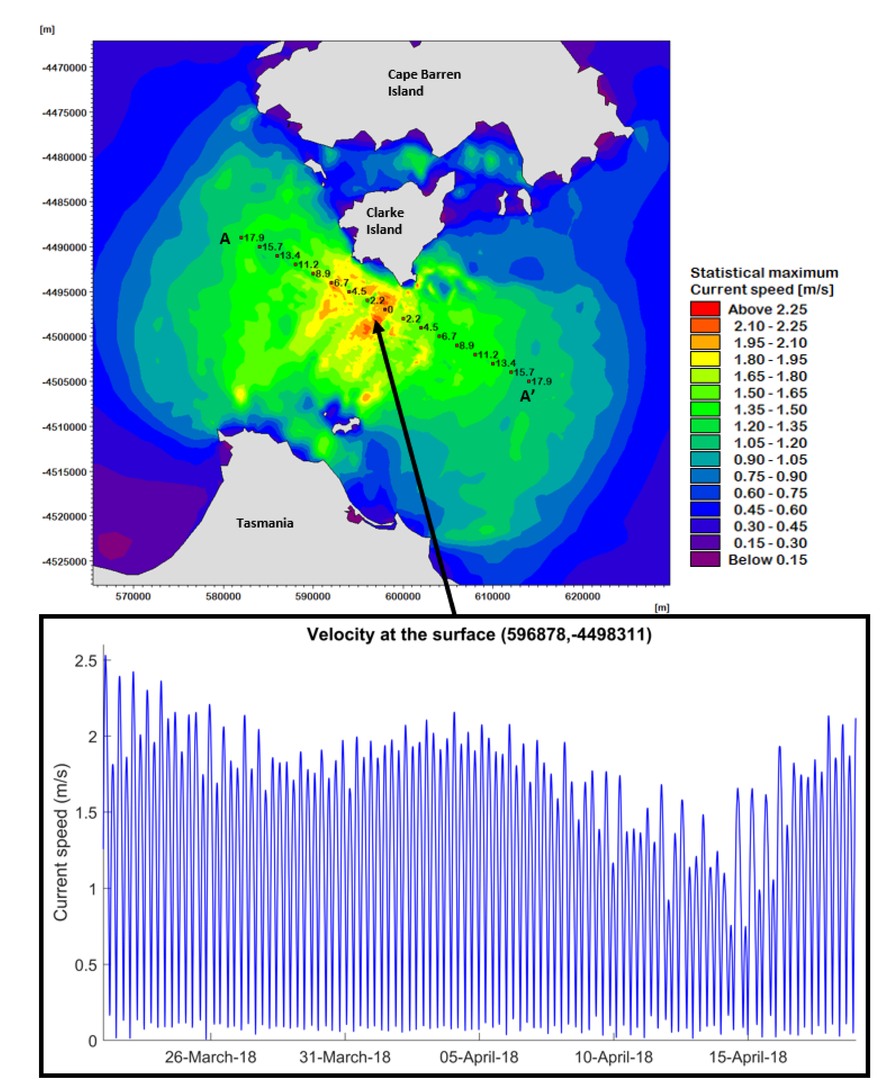
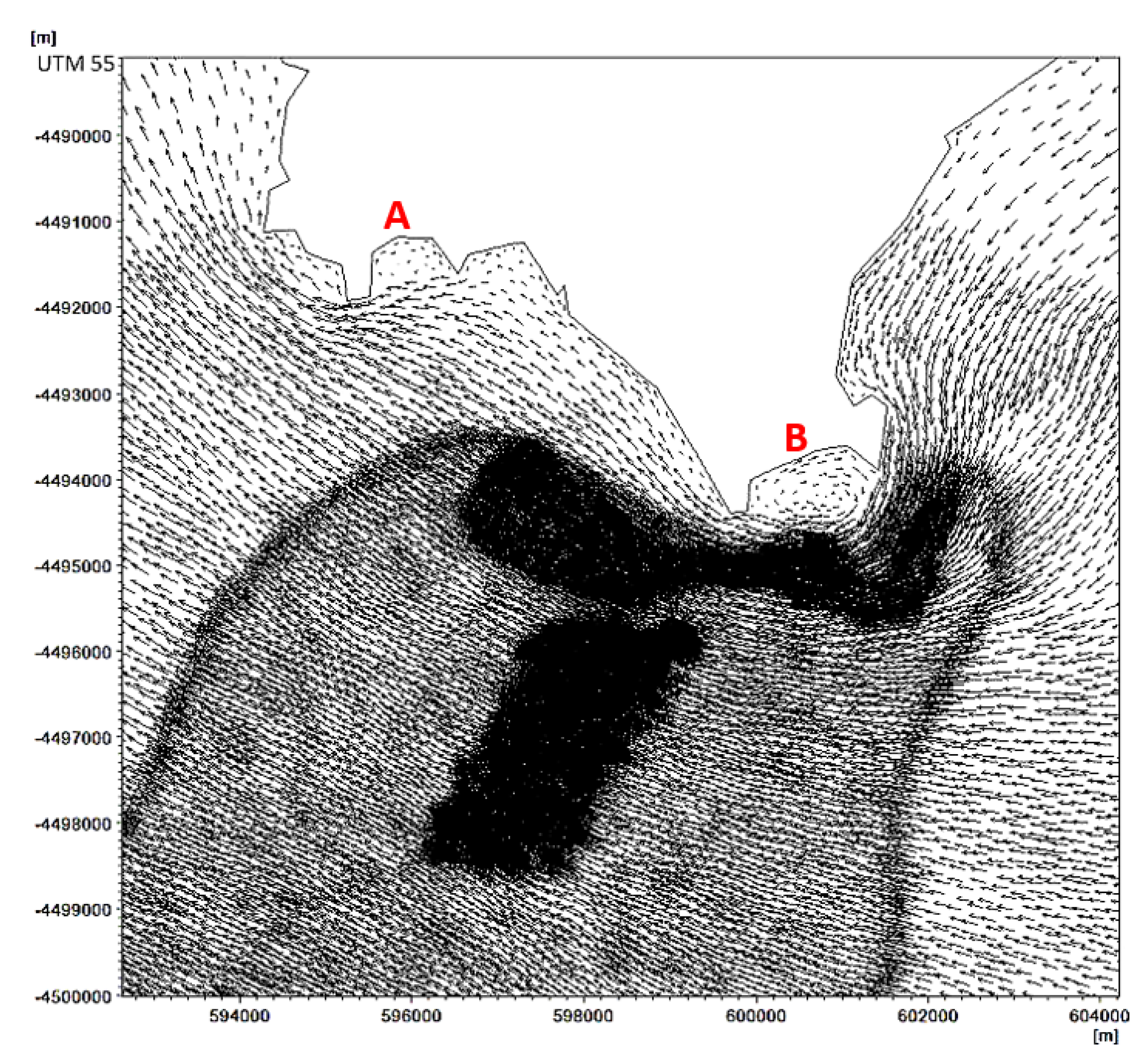
3.2. The Hydrodynamics in Banks Strait: Baseline Results
4. Influence of the Tidal Farms on the Hydrodynamics
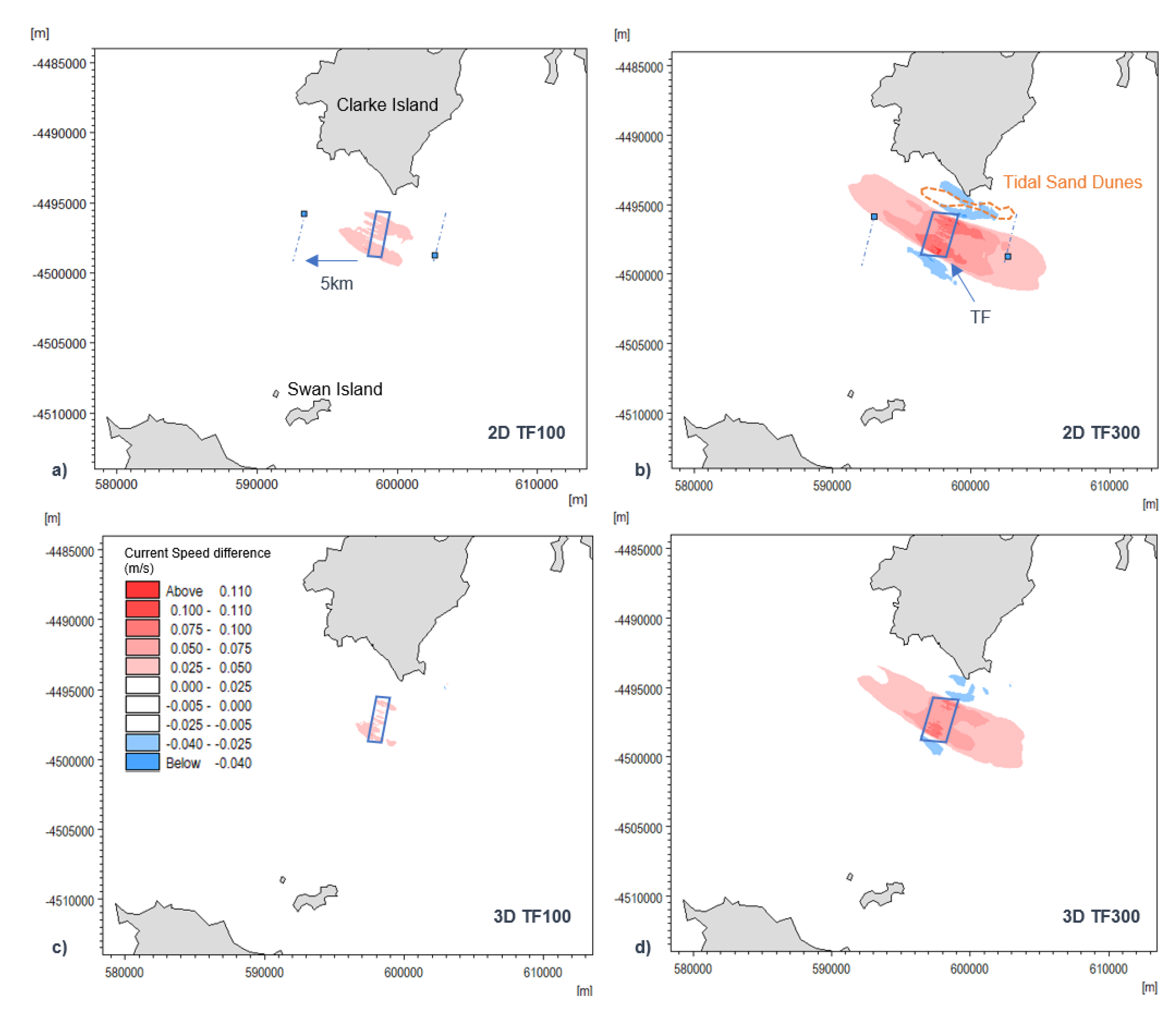
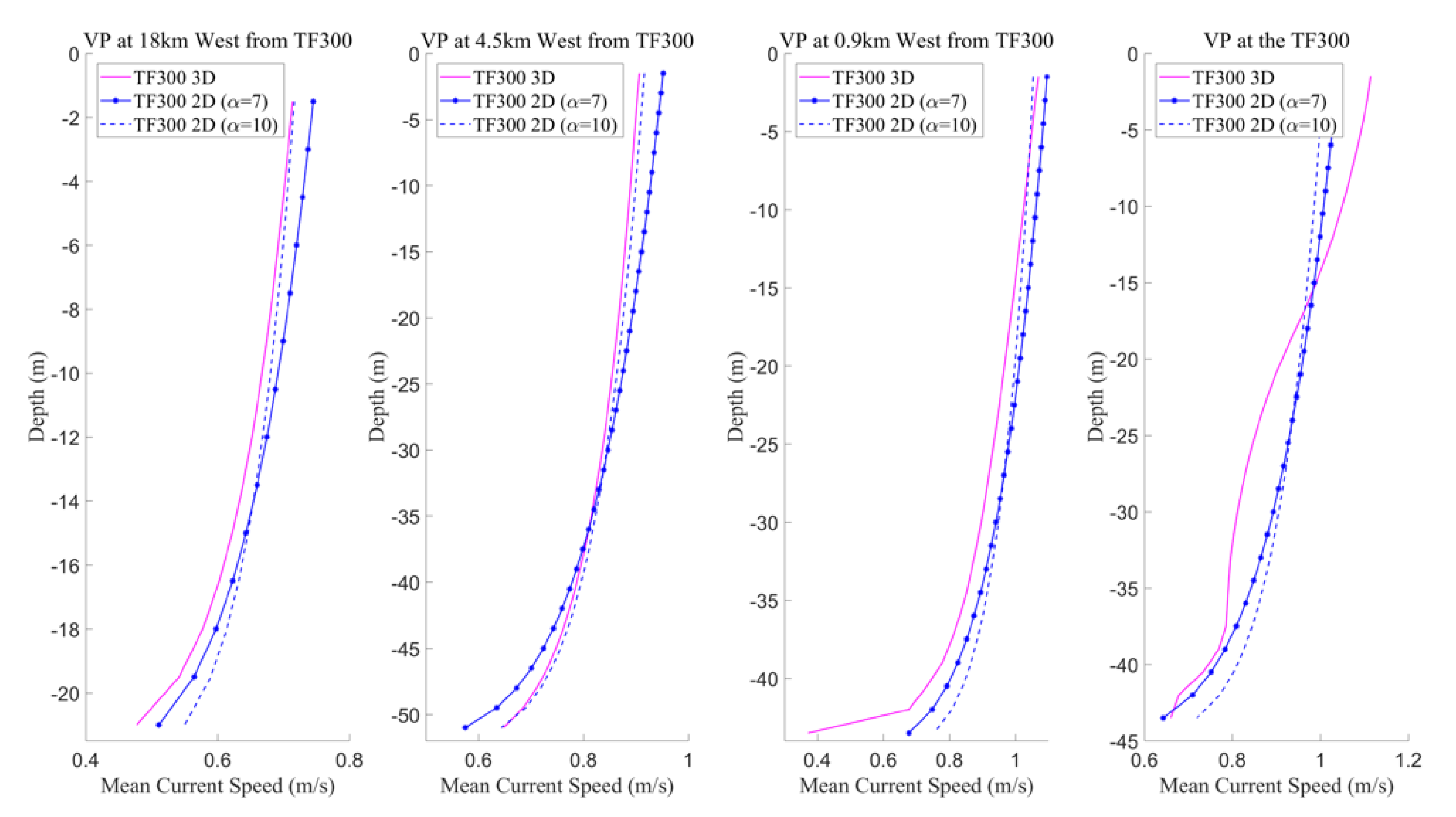
4.1. Comparison of Model Spatial Extent 2D/3D
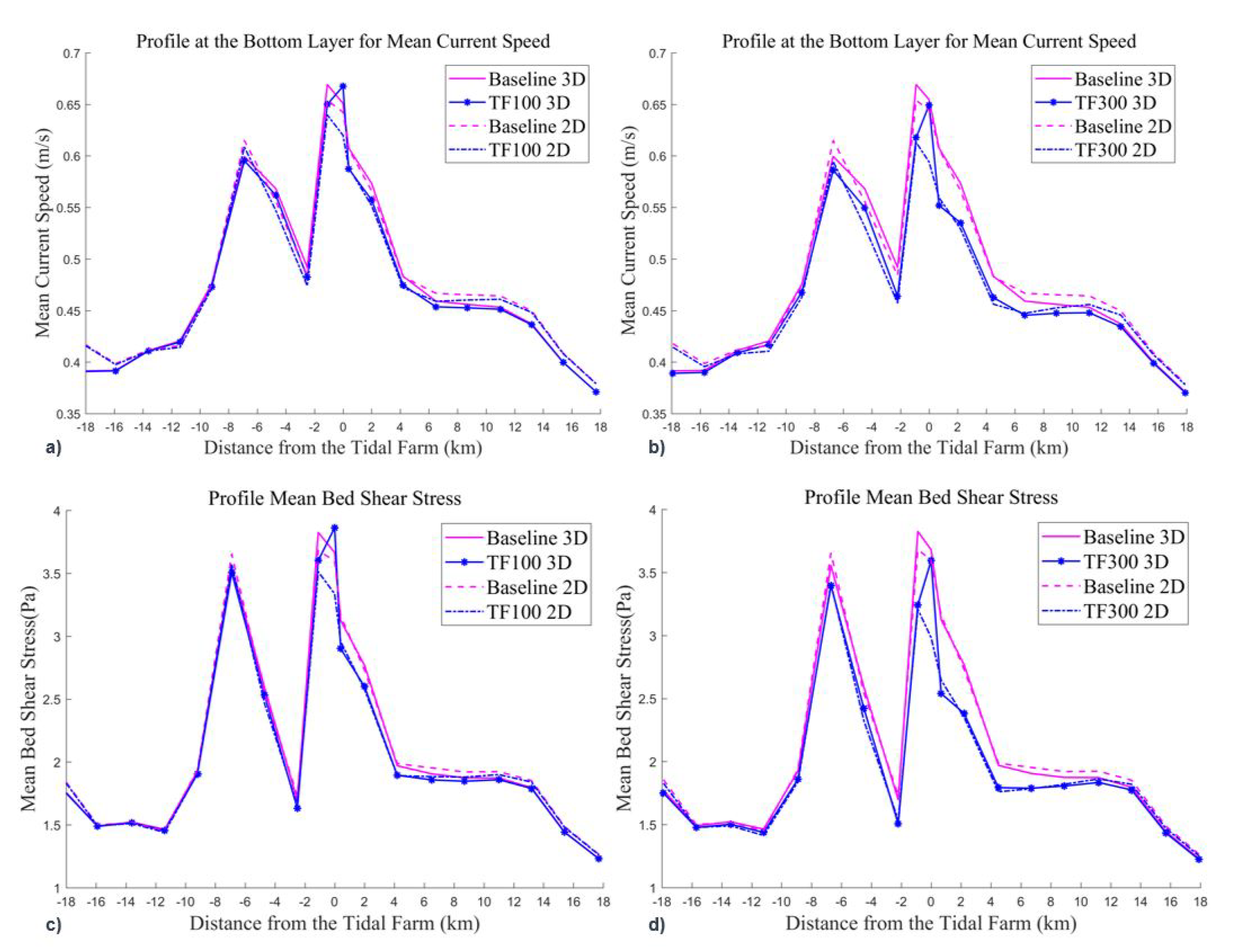
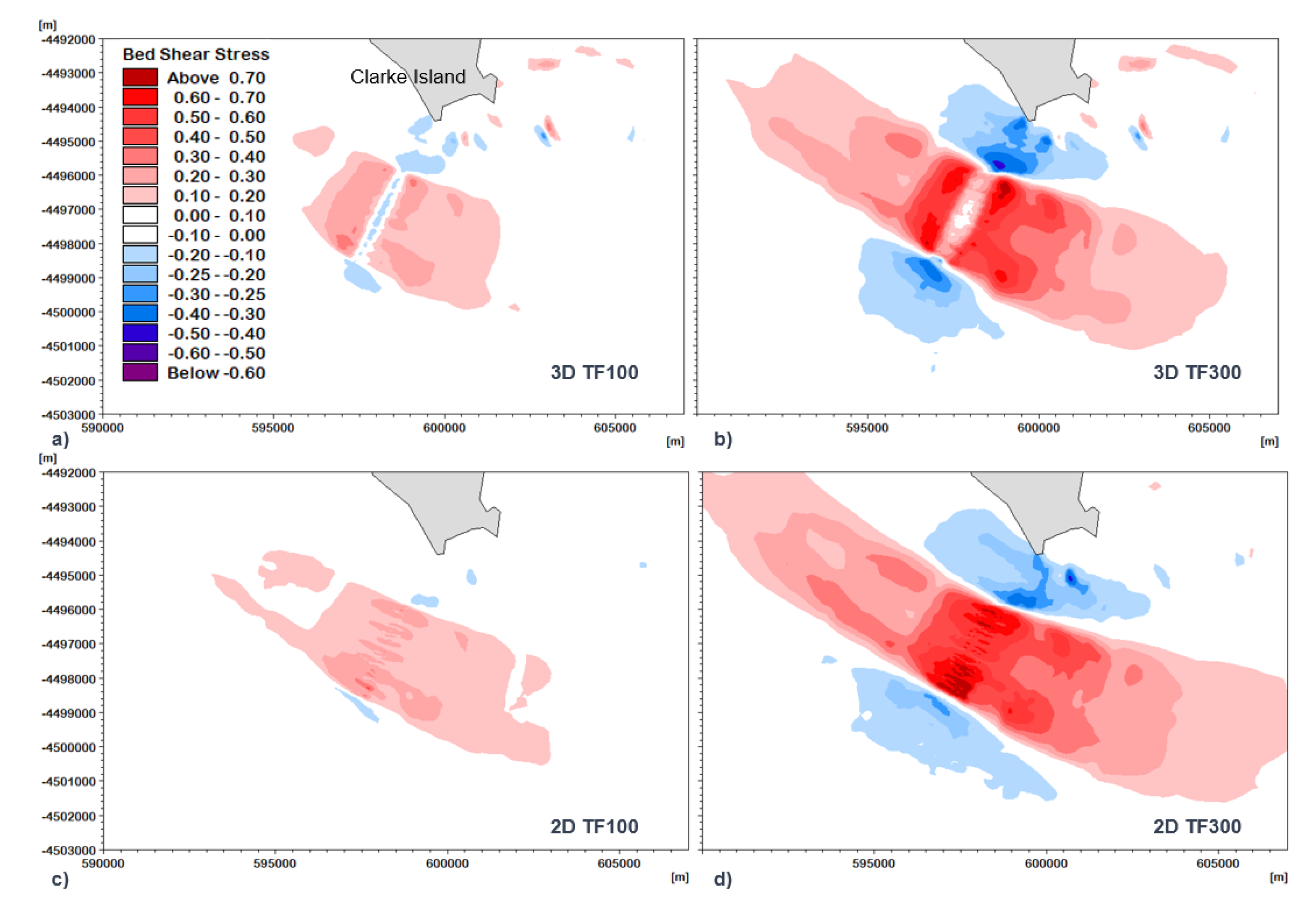
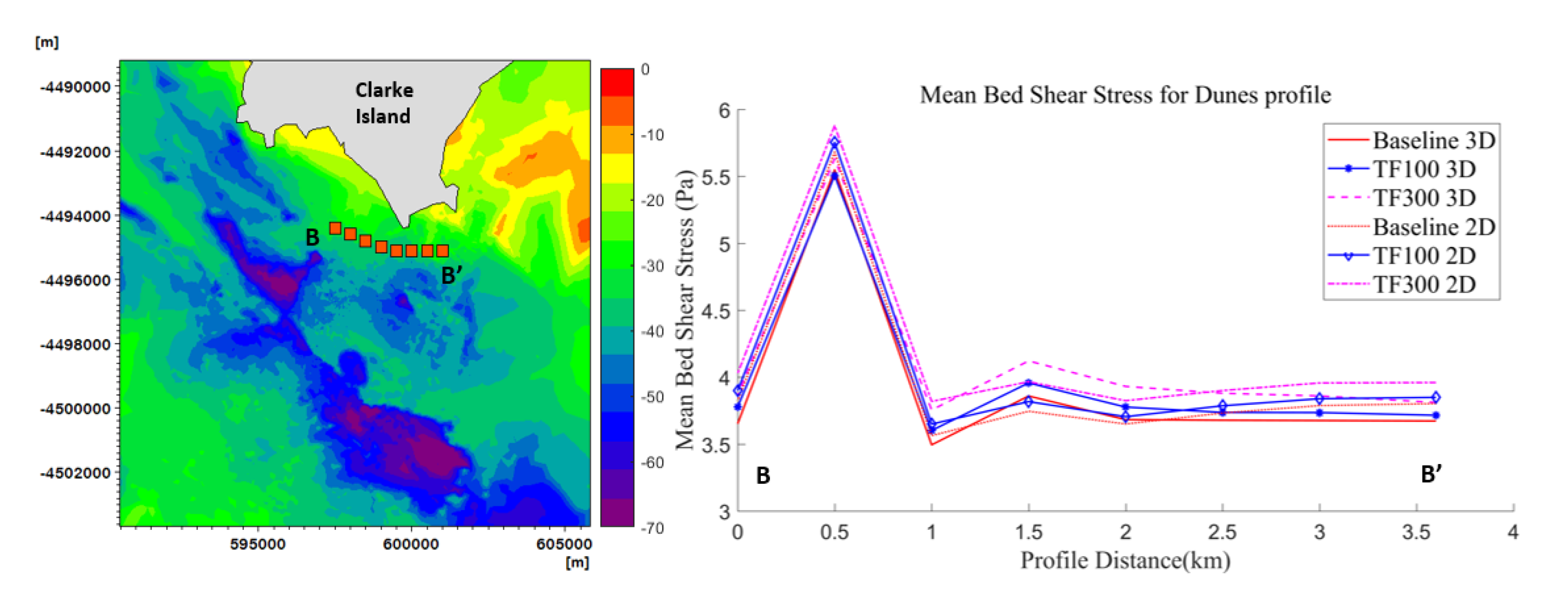
4.2. Influence Near the Seabed
5. Conclusions
Author Contributions
Funding
Acknowledgments
Conflicts of Interest
Abbreviations
| ADCP | Acoustic Doppler Current Profiler |
| AEP | Annual Energy Production |
| AHS | Australian Hydrography Service |
| ARENA | Australian Renewable Energy Agency |
| AUSTEn | Australian Tidal Energy |
| AWAC | Acoustic Waves And Current Profiler |
| CSIRO | Commonwealth Scientific and Industrial Research Organisation |
| CTD | Conductivity Temperature Depth |
| DAV | Depth Average Velocities |
| EIA | Environmental Impact Assessment |
| EMEC | European Marine Energy Centre |
| IEC | International Electrotechnical Commission |
| IMOS | Integrated Marine Observing System |
| TF | Tidal Farm |
References
- OES. Ocean Energy System Annual Report: An Overview of Ocean Energy Activities in 2019; OES: Paris, France, 2019. [Google Scholar]
- Neill, S.P.; Litt, E.J.; Couch, S.J.; Davies, A.G. The impact of tidal stream turbines on large-scale sediment dynamics. Renew. Energy 2009, 34, 2803–2812. [Google Scholar] [CrossRef]
- Frid, C.; Andonegi, E.; Depestele, J.; Judd, A.; Rihan, D.; Rogers, S.I.; Kenchington, E. The environmental interactions of tidal and wave energy generation devices. Environ. Impact Assess. Rev. 2012, 32, 133–139. [Google Scholar] [CrossRef]
- Martin-Short, R.; Hill, J.; Kramer, S.; Avdis, A.; Allison, P.; Piggott, M. Tidal resource extraction in the Pentland Firth, UK: Potential impacts on flow regime and sediment transport in the Inner Sound of Stroma. Renew. Energy 2015, 596–607. [Google Scholar] [CrossRef]
- Thiébot, J.; Bailly du Bois, P.; Guillou, S. Numerical modeling of the effect of tidal stream turbines on the hydrodynamics and the sediment transport—Application to the Alderney Race (Raz Blanchard), France. Renew. Energy 2015, 75, 356–365. [Google Scholar] [CrossRef]
- Fairley, I.; Masters, I.; Karunarathna, H. The cumulative impact of tidal stream turbine arrays on sediment transport in the Pentland Firth. Renew. Energy 2015, 80, 755–769. [Google Scholar] [CrossRef]
- Haverson, D.; Bacon, J.; Smith, H.C.; Venugopal, V.; Xiao, Q. Modelling the hydrodynamic and morphological impacts of a tidal stream development in Ramsey Sound. Renew. Energy 2018, 126, 876–887. [Google Scholar] [CrossRef]
- Robins, P.E.; Neill, S.P.; Lewis, M.J. Impact of tidal-stream arrays in relation to the natural variability of sedimentary processes. Renew. Energy 2014, 72, 311–321. [Google Scholar] [CrossRef]
- Neill, S.P.; Hashemi, M.R.; Lewis, M.J. Tidal energy leasing and tidal phasing. Renew. Energy 2016, 85, 580–587. [Google Scholar] [CrossRef]
- Ahmadian, R.; Falconer, R.A. Assessment of array shape of tidal stream turbines on hydro-environmental impacts and power output. Renew. Energy 2012, 44, 318–327. [Google Scholar] [CrossRef]
- Neill, S.P.; Jordan, J.R.; Couch, S.J. Impact of tidal energy converter (TEC) arrays on the dynamics of headland sand banks. Renew. Energy 2012, 37, 387–397. [Google Scholar] [CrossRef]
- Gallego, A.; Side, J.; Baston, S.; Waldman, S.; Bell, M.; James, M.; Davies, I.; O’Hara Murray, R.; Heath, M.; Sabatino, A.; et al. Large scale three-dimensional modelling for wave and tidal energy resource and environmental impact: Methodologies for quantifying acceptable thresholds for sustainable exploitation. Ocean Coast. Manag. 2017, 147, 67–77. [Google Scholar] [CrossRef]
- Goward Brown, A.J.; Neill, S.P.; Lewis, M.J. Tidal energy extraction in three-dimensional ocean models. Renew. Energy 2017, 114, 244–257. [Google Scholar] [CrossRef]
- Manasseh, R.; McInnes, K.L.; Hemer, M.A. Pioneering developments of marine renewable energy in Australia. Int. J. Ocean Clim. Syst. 2017, 8, 50–67. [Google Scholar] [CrossRef]
- AUSTeN. Australian Tidal Energy. 2017. Available online: http://austen.org.au/ (accessed on 30 November 2019).
- Penesis, I.; Hemer, M.; Cossu, R.; Hayward, J.; Nader, J.R.; Rosebrock, U.; Grinham, A.; Sayeef, S.; Osman, P.; Marsh, P.; et al. Tidal energy in Australia—Assessing resource and feasibility to Australia’s future energy mix. In Proceedings of the 4th Asian Wave and Tidal Energy Conference, Taipei, Taiwan, 9–13 September 2018; p. 507. [Google Scholar]
- Behrens, S.; Griffin, D.; Hayward, J.; Hemer, M.; Knight, C.; McGarry, S.; Osman, P.; Wright, J. Ocean Renewable Energy: 2015–2050: An analysis of ocean energy in Australia. North Ryde CSIRO 2012. [Google Scholar] [CrossRef]
- Marsh, P.; Penesis, I.; Nader, J.R.; Couzi, C.; Cossu, R. Assessment of tidal current resources in Banks. In Proceedings of the 13th European Wave and Tidal Energy Conference, Napoli, Italy, 1–6 September 2019; pp. 1–10. [Google Scholar]
- Wijeratne, E.M.; Pattiaratchi, C.B.; Eliot, M.; Haigh, I.D. Tidal characteristics in Bass Strait, south-east Australia. Estuar. Coast. Shelf Sci. 2012, 114, 156–165. [Google Scholar] [CrossRef]
- Sandery, P.A.; Kämpf, J. Winter-Spring flushing of Bass Strait, South-Eastern Australia: A numerical modelling study. Estuar. Coast. Shelf Sci. 2005, 63, 23–31. [Google Scholar] [CrossRef]
- Sandery, P.A.; Kämpf, J. Transport timescales for identifying seasonal variation in Bass Strait, south-eastern Australia. Estuar. Coast. Shelf Sci. 2007, 74, 684–696. [Google Scholar] [CrossRef]
- McIntosh, P.C.; Bennett, A.F. Open Ocean Modeling as an Inverse Problem: M 2 Tides in Bass Strait. J. Phys. Oceanogr. 1984, 14, 601–614. [Google Scholar] [CrossRef]
- McInnes, K.L.; O’Grady, J.G.; Hemer, M.; Macadam, I.; Abbs, D.J.; White, C.J.; Corney, S.P.; Grose, M.R.; Holz, G.K.; Gaynor, S.M.; et al. Climate Futures for Tasmania: Extreme Tide and Sea-Level Events Technical Report; Technical Report January; Antarctic Climate and Ecosystems Cooperative Research Centre: Hobart, Tasmania, 2011. [Google Scholar]
- Fandry, C.B. Development of a Numerical Model of Tidal and Wind-driven Circulation in Bass Strait. Mar. Freshw. Res. 1981, 32, 9–29. [Google Scholar] [CrossRef]
- Fandry, C.B.; Hubbert, G.D.; McIntosh, P.C. Comparison of predictions of a numerical model and observations of tides in bass strait. Mar. Freshw. Res. 1985, 36, 737–752. [Google Scholar] [CrossRef]
- Wijffels, S.E.; Beggs, H.; Griffin, C.; Middleton, J.F.; Cahill, M.; King, E.; Jones, E.; Feng, M.; Benthuysen, J.A.; Steinberg, C.R.; et al. A fine spatial-scale sea surface temperature atlas of the Australian regional seas (SSTAARS): Seasonal variability and trends around Australasia and New Zealand revisited. J. Mar. Syst. 2018, 187, 156–196. [Google Scholar] [CrossRef]
- Fortunato, A.B.; Bertin, X.; Oliveira, A. Space and time variability of uncertainty in morphodynamic simulations. Coast. Eng. 2009, 56, 886–894. [Google Scholar] [CrossRef]
- Pinto, L.; Fortunato, A.B.; Freire, P. Sensitivity analysis of non-cohesive sediment transport formulae. Cont. Shelf Res. 2006, 26, 1826–1839. [Google Scholar] [CrossRef]
- Nash, S.; Phoenix, A. A review of the current understanding of the hydro-environmental impacts of energy removal by tidal turbines. Renew. Sustain. Energy Rev. 2017, 80, 648–662. [Google Scholar] [CrossRef]
- Galibert, G. IMOS Toolbox Version 2.x.x. 2020. Available online: https://github.com/aodn/imos-toolbox (accessed on 21 March 2019).
- Scherelis, C.; Penesis, I.; Marsh, P.; Cossu, R.; Hemer, M.; Wright, J. Relating fish distributions to physical characteristics of a tidal energy candidate site in the Banks Strait Australia. In Proceedings of the 13th European Wave and Tidal Energy Conference, Napoli, Italy, 1–6 September 2019; pp. 1–8. [Google Scholar]
- Perez, L.; Cossu, R.; Couzi, C.; Penesis, I. Wave-Turbulence Decomposition Methods Applied to Tidal Energy Site Assessment. Energies 2020, 13, 1245. [Google Scholar] [CrossRef]
- Coles, D.S.; Blunden, L.S.; Bahaj, A.S. Assessment of the energy extraction potential at tidal sites around the Channel Islands. Energy 2017, 124, 171–186. [Google Scholar] [CrossRef]
- DHI. MIKE 21 & MIKE 3 Flow Model FM, Hydrodynamic Module Scientific Documentation; DHI: Hesholm, Denmark, 2017. [Google Scholar]
- Whiteway, T. Australian Bathymetry and Topography Grid. Geosci. Aust. Canberra 2009. [Google Scholar] [CrossRef]
- Australian Hydrographic Office Charts. Available online: http://www.hydro.gov.au/prodserv/paper/auspapercharts.htm (accessed on 1 March 2018).
- Yongcun, C.; Ole Baltazar, A. Improvement in global ocean tide model in shallow water regions, 2010. In Proceedings of the OSTST, Lisbon, Portugal, 18–22 October 2010. [Google Scholar]
- International Electrotechnical Commission. IEC/TS 62600-201: Marine Energy—Wave, Tidal and Other Water Current Converters and Characterization; International Electrotechnical Committee: Genova, Switzerland, 2015. [Google Scholar]
- Copernicus Climate Change Service (C3S). ERA5: Fifth generation of ECMWF Atmospheric Reanalyses of the Global Climate. Copernicus Climate Change Service Climate Data Store (CDS). 2017. Available online: https://cds.climate.copernicus.eu/cdsapp#!/home (accessed on 5 January 2019).
- Swan Island: Tasmania Daily Weather Observations. Available online: http://www.bom.gov.au/climate/dwo/IDCJDW7051.latest.shtml (accessed on 5 January 2019).
- Soulsby, R. Dynamics of Marine Sands; Thomas Telford Publishing: London, UK, 1997; Available online: https://www.icevirtuallibrary.com/doi/pdf/10.1680/doms.25844 (accessed on 5 January 2018). [CrossRef]
- Waldman, S.; Bastón, S.; Nemalidinne, R.; Chatzirodou, A.; Venugopal, V.; Side, J. Implementation of tidal turbines in MIKE 3 and Delft3D models of Pentland Firth & Orkney Waters. Ocean Coast. Manag. 2017, 147, 21–36. [Google Scholar] [CrossRef]
- EMEC Orkney. Environmental Impact Assessment (EIA). Guidance for Developers at the European Marine Energy Centre; Technical Report; EMEC Orkney: Stromness, UK, 2008. [Google Scholar]
- Thiébot, J.; Guillou, N.; Guillou, S.; Good, A.; Lewis, M. Wake field study of tidal turbines under realistic flow conditions. Renew. Energy 2020, 151, 1196–1208. [Google Scholar] [CrossRef]
- Lewis, M.; Neill, S.; Robins, P.; Hashemi, M.; Ward, S. Characteristics of the velocity profile at tidal-stream energy sites. Renew. Energy 2017, 114, 258–272. [Google Scholar] [CrossRef]
- Gunn, K.; Stock-Williams, C. On validating numerical hydrodynamic models of complex tidal flow. Int. J. Mar. Energy 2013, 3–4, e82–e97. [Google Scholar] [CrossRef]
- Sellar, B.; Wakelam, G. Characterisation of Tidal Flows at the European Marine Energy Centre in the Absence of Ocean Waves. Energies 2018, 11, 176. [Google Scholar] [CrossRef]
- Codiga, D. UTide Unified Tidal Analysis and Prediction Functions. MATLAB Central File Exchange. 2020. Available online: https://www.mathworks.com/matlabcentral/fileexchange/46523-utide-unified-tidal-analysis-and-prediction-functionsl (accessed on 22 January 2020).
- Australian Baseline Sea Level Monitoring Project Hourly Sea Level and Meteorological Data. Available online: http://www.bom.gov.au/oceanography/projects/abslmp/data/index.shtml (accessed on 1 March 2018).
- Hagerman, G.; Polagye, B.; Bedard, R.; Previsic, M. Methodology for Estimating Tidal Current Energy Resources and Power Production by Tidal In-Stream Energy Conversion (TISEC) Devices; EPRI North American Tidal In Stream Power Feasibility Demonstration Project, 2006. Available online: https://tethys.pnnl.gov/sites/default/files/publications/Tidal_Current_Energy_Resources_with_TISEC.pdf (accessed on 22 January 2020).
- Gooch, S.; Thomson, J.; Polagye, B.; Meggitt, D. Site characterization for tidal power. In Proceedings of the OCEANS 2009, Venice, Italy, 21–25 September 2009; pp. 1–10. [Google Scholar]
- O’Rourke, F.; Boyle, F.; Reynolds, A. Ireland’s tidal energy resource; An assessment of a site in the Bulls Mouth and the Shannon Estuary using measured data. Energy Convers. Manag. 2014, 87, 726–734. [Google Scholar] [CrossRef]
- Gunn, K.; Stock-Williams, C. Fall of Warness 3D Model Validation Report: ETI REDAPT MA1001 PM14 MD5.2; Technical Report; E.ON New Build Technology: Coventry, UK, 2012. [Google Scholar]
- Dyer, K.R.; Huntley, D.A. The origin, classification and modelling of sand banks and ridges. Cont. Shelf Res. 1999, 19, 1285–1330. [Google Scholar] [CrossRef]
- Gibbs, C.; Tomczak, M.; Longmore, A. The Nutrient Regime of Bass Strait. Mar. Freshw. Res. 1986, 37, 451–466. [Google Scholar] [CrossRef]


| Location | Year | Device Type | Company | Power Rating | Indicative Depth |
|---|---|---|---|---|---|
| of Operation (m) | |||||
| Darwin | 1996 | Tyson Turbine fluted cone axial turbine (pontoon) | Northern Territory University (NTU) | <1 kW | 1 |
| Darwin | 1998 | NTU Swenson axial turbine (pontoon) | NTU | 2.2 kW | 1–2 |
| King Sound | 2000– 2014 | Barrage dam investigation | Tidal Energy Australia and Hydro Tasmania | 40 MW | ∖ |
| Clarence river | 2004 | Aquanator reaction plates in closed loop track | Atlantis Energy Ltd | 5 kW | 2 |
| San Remo | 2006 | Aquanator | Atlantis Resources | 100 kW | 2 |
| San Remo | 2007 | Submersible tidal generator | HydroGen Power Industries | 5–50 kW | up to 20 |
| Brisbane | 2007 | Submersible tidal generator | HydroGen Power Industries | 5–50 kW | up to 20 |
| San Remo/ Stony Point | 2008 | Floating tidal turbine laboratory | EnGen Institute | ∖ | 2 |
| Corio Bay | 2008 | Solon ducted axial turbine | Atlantis Resources | 160 kW | 10 |
| Melbourne | 2009 | 3D printed multi-axis turbine array | Cetus | 1 kW | 1 |
| Newcastle | 2012 | Sea Urchin axial turbine (pontoon) | Elementary Energy Tech. | 2 kW | 1–2 |
| San Remo | 2012 | Cross-flow turbine tidal desalination | Infra Tidal | 15 kW | 2.5 |
| Tamar Estuary | 2016 | Ducted axial turbine (pontoon) | Mako | 10 kW | 2 |
| Gladstone port | 2018 | Ducted axial turbine | Mako | ∖ | ∖ |
| Name Station | Type of Instrument | Longitude | Latitude | Depth (m) | Date of Deployment | End of Data Collected | Cell Size (m) | Length (Days) |
|---|---|---|---|---|---|---|---|---|
| CW2 | RDI Sentinel V50 500 k Hz | 148.10188 | −40.5848 | 46.47 | 22/03/2018 | 11/07/2018 | 0.5 | 110 |
| C1 | RDI Workshorse 300 k Hz | 148.23882 | −40.6727 | 57.94 | 17/03/2018 | 10/07/2018 | 2.0 | 115 |
| CW3 | Nortek AWAC 1 M Hz | 148.07778 | −40.5454 | 34.95 | 22/03/2018 | 16/06/2018 | 0.5 | 86 |
| CW4 | Nortek AWAC 1 M Hz | 148.09241 | −40.6664 | 30.67 | 15/03/2018 | 09/06/2018 | 1.0 | 85 |
| CWTb1 | Nortek Signature 500 k Hz | 148.22626 | −40.6672 | 63.57 | 22/03/2018 | 09/07/2018 | 1.0 | 109 |
| CW1 | RDI Sentinel V50 500 Hz | 148.05684 | −40.5294 | 27.11 | 12/07/2018 | 06/09/2018 | 0.5 | 57 |
| CW2 bis | RDI Sentinel V50 500 Hz | 148.20132 | −40.701 | 46.08 | 12/07/2018 | 22/09/2018 | 0.5 | 72 |
| CW4bis | Nortek AWAC 1 M Hz | 148.34497 | −40.7296 | 25.42 | 13/07/2018 | 08/09/2018 | 1.0 | 54 |
| C1 bis | RDI Workshorse 300 k Hz | 148.12498 | −40.6891 | 29.07 | 05/12/2018 | 15/02/2019 | 1.0 | 72 |
| Phase for M2 (degree) | Amplitude for M2 (m) | |||||||||
|---|---|---|---|---|---|---|---|---|---|---|
| 3D | 2D | 3D | 2D | |||||||
| Stations | OBS | R4 | R9 | R4 | R9 | OBS | R4 | R9 | R4 | R9 |
| CW2 | 140 | 139 | 139 | 139 | 139 | 1.25 | 1.3 | 1.25 | 1.38 | 1.31 |
| CW3 | 118 | 125 | 125 | 125 | 125 | 0.99 | 0.97 | 0.93 | 1.03 | 0.97 |
| CW4 | 161 | 165 | 165 | 165 | 165 | 1.36 | 1.3 | 1.23 | 1.38 | 1.29 |
| C1 | 165 | 158 | 157 | 157 | 157 | 0.85 | 0.88 | 0.85 | 0.93 | 0.89 |
| CWTb1 | 158 | 154 | 153 | 154 | 153 | 0.88 | 0.91 | 0.88 | 0.96 | 0.92 |
| Difference in DAV | ||||
|---|---|---|---|---|
| TF300 | TF100 | |||
| Distance From Tidal Farm (km) | 3D | 2D | 3D | 2D |
| 0 | 7.39% | 8.44% | 3.67% | 3.69% |
| 4.5 | 4.06% | 5.21% | 1.55% | 1.94% |
| 9 | 2.05% | 2.64% | 0.73% | 0.92% |
| 13.4 | 0.67% | 0.92% | 0.19% | 0.31% |
| 18 (towards Bass Strait) | 0.62% | 0.84% | 0.18% | 0.26% |
| 18 (towards Tasman Sea) | 0.21% | 0.35% | 0% | 0% |
© 2020 by the authors. Licensee MDPI, Basel, Switzerland. This article is an open access article distributed under the terms and conditions of the Creative Commons Attribution (CC BY) license (http://creativecommons.org/licenses/by/4.0/).
Share and Cite
Auguste, C.; Marsh, P.; Nader, J.-R.; Cossu, R.; Penesis, I. Towards a Tidal Farm in Banks Strait, Tasmania: Influence of Tidal Array on Hydrodynamics. Energies 2020, 13, 5326. https://doi.org/10.3390/en13205326
Auguste C, Marsh P, Nader J-R, Cossu R, Penesis I. Towards a Tidal Farm in Banks Strait, Tasmania: Influence of Tidal Array on Hydrodynamics. Energies. 2020; 13(20):5326. https://doi.org/10.3390/en13205326
Chicago/Turabian StyleAuguste, Christelle, Philip Marsh, Jean-Roch Nader, Remo Cossu, and Irene Penesis. 2020. "Towards a Tidal Farm in Banks Strait, Tasmania: Influence of Tidal Array on Hydrodynamics" Energies 13, no. 20: 5326. https://doi.org/10.3390/en13205326
APA StyleAuguste, C., Marsh, P., Nader, J.-R., Cossu, R., & Penesis, I. (2020). Towards a Tidal Farm in Banks Strait, Tasmania: Influence of Tidal Array on Hydrodynamics. Energies, 13(20), 5326. https://doi.org/10.3390/en13205326