AATTENUATION—The Atmospheric Attenuation Model for CSP Tower Plants: A Look-Up Table for Operational Implementation

Abstract

Attenuation of solar radiation between the receiver and the heliostat field in concentrated solar power (CSP) tower plants can reduce the overall system performance significantly. The attenuation varies strongly with time and the average attenuation at different sites might also vary strongly from each other. If no site specific attenuation data is available, the optimal plant design cannot be determined and rough estimations of the attenuation effect are required leading to high uncertainties of yield analysis calculations. The attenuation is caused mainly by water vapor content and aerosol particles in the lower atmospheric layer above ground. Although several on-site measurement systems have been developed during recent years, attenuation data sets are usually not available to be included during the plant project development. An Atmospheric Attenuation (AATTENUATION) model to derive the atmospheric transmittance between a heliostat and receiver on the basis of common direct normal irradiance (DNI), temperature, relative humidity, and barometric pressure measurements was developed and validated by the authors earlier. The model allows the accurate estimation of attenuation for sites with low attenuation and gives an estimation of the attenuation for less clear sites. However, the site-dependent coefficients of the AATTENUATION model had to be developed individually for each site of interest, which required time-consuming radiative transfer simulations, considering the exact location and altitude, as well as the pre-dominant aerosol type at the location. This strongly limited the application of the model despite its typically available input data. In this manuscript, a look-up table (LUT) is presented which enables the application of the AATTENUATION model at the site of interest without the necessity to perform the according complex radiative transfer calculations for each site individually. This enables the application of the AATTENUATION model for virtually all resource assessments for tower plants and in an operational mode in real time within plant monitoring systems around the world. The LUT also facilitates the generation of solar attenuation maps on the basis of long-term meteorological data sets which can be considered during resource assessment for CSP tower plant projects. The LUTs are provided together with this manuscript as supplementary files. The LUT for the AATTENUATION model was developed for a solar zenith angle (SZA) grid of 1°, an altitude grid of 100 m, 7 different standard aerosol types and the standard AFGL atmospheres for mid-latitudes and the tropics. The LUT was tested against the original version of the AATTENUATION model at 4 sites in Morocco and Spain, and it was found that the additional uncertainty introduced by the application of the LUT is negligible. With the information of latitude, longitude, altitude above mean sea level, DNI, relative humidity (RH), ambient temperature ($T_{air}$), and barometric pressure (bp), the attenuation can be now derived easily for each site of interest.

1. Introduction

The design and operation of CSP technologies have to be optimized for the site-dependent conditions so that their potential can be exploited ideally. In regions with high solar radiation levels reaching the surface, e.g., the Middle East and northern African (MENA) region or Southern Europe, a strong potential for solar energy production faces challenging environmental conditions the power plants are exposed to. This area is dominated by arid or semi-arid conditions, e.g., the African Sahara, which is, for example, the primary source for mineral dust particles released to the atmosphere [1]. In CSP central tower plants, a heliostat field focuses the solar irradiance which reaches the ground level onto a receiver on the top of a tower.

Atmospheric extinction over a slant path is the partial loss or attenuation of by the heliostat field reflected radiation on its path to the central receiver. The distance between the heliostat field and the central receiver can be up to a few kilometers [2,3,4]; therefore, this phenomenon cannot be neglected during plant yield assessment, as well as during operation and for the design of a CSP tower plant. An example for the influence in horizontal atmospheric attenuation on an exemplary CSP tower plant with a design thermal power of 162 $M{W}_{th}$, a storage capacity of 12 h and a molten salt receiver is evaluated in Reference [5]. It could be found that, for this exemplary plant, the annual plant yield is reduced by about 1.56% if overload dumping is considered and around 7% if it is not considered. Therefore, several on-site measurement systems have been developed in the past (summarized in References [5,6]). Atmospheric extinction varies with site and time and is important at sites with high aerosol loads and/or water vapor content. This is, therefore, especially important at arid sites, e.g., the Middle East and northern African (MENA) region, where CSP will play a strong role in the electricity market [7]. As most on-site measurement methods to consider the atmospheric extinction are only applied rarely due to their complexity within the project planning process, in many cases, only one of two standard cases, e.g., typical clear or typical hazy, is considered [5]. This can lead to under- or over-estimations of several percent in terms of the expected annual plant yield [5,8,9]. On-site attenuation conditions should be considered to further reduce risk margins, which are usually included in yield calculations of engineering, procurement and construction (EPC) contractors and, therefore, to reduce the price of solar tower plants. As a large share of the overall costs is caused by the heliostat field [10,11], the density of the heliostat field must be selected site specific as a tradeoff between land costs and solar extinction, on the one hand, and blocking and shading losses causes by neighboring heliostats. Optimally designed plants for the local conditions of the site are necessary to reach the lowest energy prices.

Usually, meteorological data sets, including irradiance measurements or typical meteorological years, are acquired within the planning phase for a CSP project. As it is not always possible to also perform on-site measurements of the atmospheric extinction additionally to the standard measurement setup during the resource assessment process, the need of according modeling methods arose during the last few years, and different methods have been presented [12,13,14,15,16,17,18]. The different models use, for example, the aerosol optical depth (AOD) of, e.g., the AERONET network, remote sensing data of MODIS, or water vapor data sets.

The proposed method to model atmospheric attenuation in solar tower plants, the so-called AATTENUATION model, has the advantage that it can be applied only with data sets of the usually already available DNI, $T_{air}$, and RH for the site of interest. The model has been validated so far for the usage of on-site ground measurements [6,19], but the AATTENUATION model can also be applied using, e.g., satellite data or data sets from other sources, taking into account that these other sources might suffer from additional uncertainties. A look-up table (LUT) and a description on how to use the AATTENUATION model together with the LUT is presented which enables a worldwide operational application of the model. The data of the LUT is provided in parallel to this manuscript.

This manuscript is structured in 5 sections. In the Section 2, the AATTENUATION model and the development of its LUT is described in detail. Section 3 includes a discussion of the LUT data set for different standard aerosol type mixtures. This section also presents the validation of the LUT in comparison to the former model which was based on individual radiative transfer calculations for each site of interest. Section 4 gives a step-by-step description on how to use the AATTENUATION model and its LUT for plant yield calculations or during plant operation. A final conclusion is given in Section 5.

2. DNI Based AATTENUATION Model Look-Up Table

2.1. AATTENUATION Model Concept

Water vapor and aerosol particles cause absorption and scattering processes which can also be referred as atmospheric extinction or attenuation of solar irradiance. Solar radiation is attenuated on its way from the top of the atmosphere to the ground due to time- and site dependent aerosol particles and water vapor concentrations. This attenuation and the according reduction of solar radiation at ground level has to be considered in solar energy resource assessment and plant yield calculations. One example model on how to estimate the column atmospheric attenuation dependent on the clearness index is described in Reference [20], addressing the calculation of the atmospheric attenuation in the whole column between the top of the atmosphere and ground level by taking into account that the attenuation is connected to the inverse of the clearness index. It discusses that the attenuation is dependent on the number or quantity of attenuators which can be described as a population. In CSP tower plants, a second effect of solar radiation attenuation takes place as the radiation is reflected by the heliostat field onto a central receiver on top of a tower. As the radiation has to cross the lower atmosphere on a slant path between the heliostat and the receiver where usually most of the aerosol particles and water vapor droplets are located, this additional attenuation cannot be neglected in, e.g., yield calculations. The attenuation between the top of the atmosphere and the ground is covered if ground radiation measurements are used for resource assessment purposes (or modeled with, e.g., the model of Reference [20]). The second attenuation effect has to be additionally measured or modeled. This manuscript deals with a model which estimated this slant path atmospheric attenuation on the basis of commonly available meteorological parameter. As already described in References [19,21], a AATTENUATION model was developed which derives the atmospheric attenuation only from DNI, RH, bp data, the SZA, and the altitude of the site of interest. We briefly summarize the main formulas of this approach, but for details please see [6,19].

The following approximation can be used to express the relation between the broadband transmittance for a slant range x ( $T_x$) and the broadband extinction coefficient ${\beta }_{ext}$:

$$T_x={\displaystyle \frac{DN{I}_B}{DN{I}_A}}\approx exp\left(-{\beta }_{ext}·x\right).$$

(1)

Here, $DN{I}_A$ (direct normal irradiance) is the incoming DNI directly after being reflected by the heliostat and $DN{I}_B$ is the DNI reflected by the heliostat reaching the central receiver after traveling through an atmospheric layer between A and B. The term “broadband” refers in this work to the wavelength range between 250 and 4000 nm.

We model the extinction coefficient ${\beta }_{ext}$ with the following formula:

$${\beta }_{ext,mod}=a·\left(-ln\left({\displaystyle \frac{DN{I}_{meas}}{DN{I}_{clean,sim}}}\right)·cos\left(SZA\right)\right)+b.$$

(2)

$DN{I}_{meas}$ is here the measured DNI at ground level, and $DN{I}_{clean,sim}$ is the simulated DNI for an aerosol-free atmosphere at ground level. The coefficients a and b are derived using radiative transfer calculations with the radiative transfer code libRadtran [22,23]. SZA is the solar zenith angle.

The atmospheric attenuation $A_x$ over a slant range x, as well as the transmittance $T_x$, can then be calculated with:

$$A_x=1-T_x=exp\left(-\left(a·\left(-ln\left({\displaystyle \frac{DN{I}_{meas}}{DN{I}_{clean,sim}}}\right)·cos\left(\vartheta \right)\right)+b\right)·x\right).$$

(3)

One main assumption of the AATTENUATION model is the vertical extinction profile assumed within the radiative transfer calculations to derive a and b. Therefore, three different assumptions of the extinction height profile were tested and validated in Reference [6]. The most promising approach is to assume a homogeneous aerosol particle distribution in the first kilometer over ground and no aerosol particles above this layer. The root mean square error (RMSE) of the broadband transmittance for a slant range of 1 km ($T_{1km}$) is calculated for this assumption to be around 5–8% for three examined sites in Morocco and Spain.

The AATTENUATION model is applied only for clear-sky conditions. To identify cloudy data points, a cloud detection algorithm was deployed which uses thresholds of the Linke turbitidy (TL) coefficient. The exact procedure on how cloudy data points are detected is described in Reference [19] and is also explained in Section 5.

With the help of $T_{air}$, bp, and the RH for each data points, the precipitable water vapor (PWV) can be derived according to the empirical equations of Reference [24,25]. The AATTENUATION model coefficients are chosen for each time step according to the PWV level. The simulated $DN{I}_{clean,sim}$ which is taken as the reference for an aerosol-free atmosphere is taken from the simulations dependent on the SZA, as well as the PWV.

2.2. Look-Up Table Development

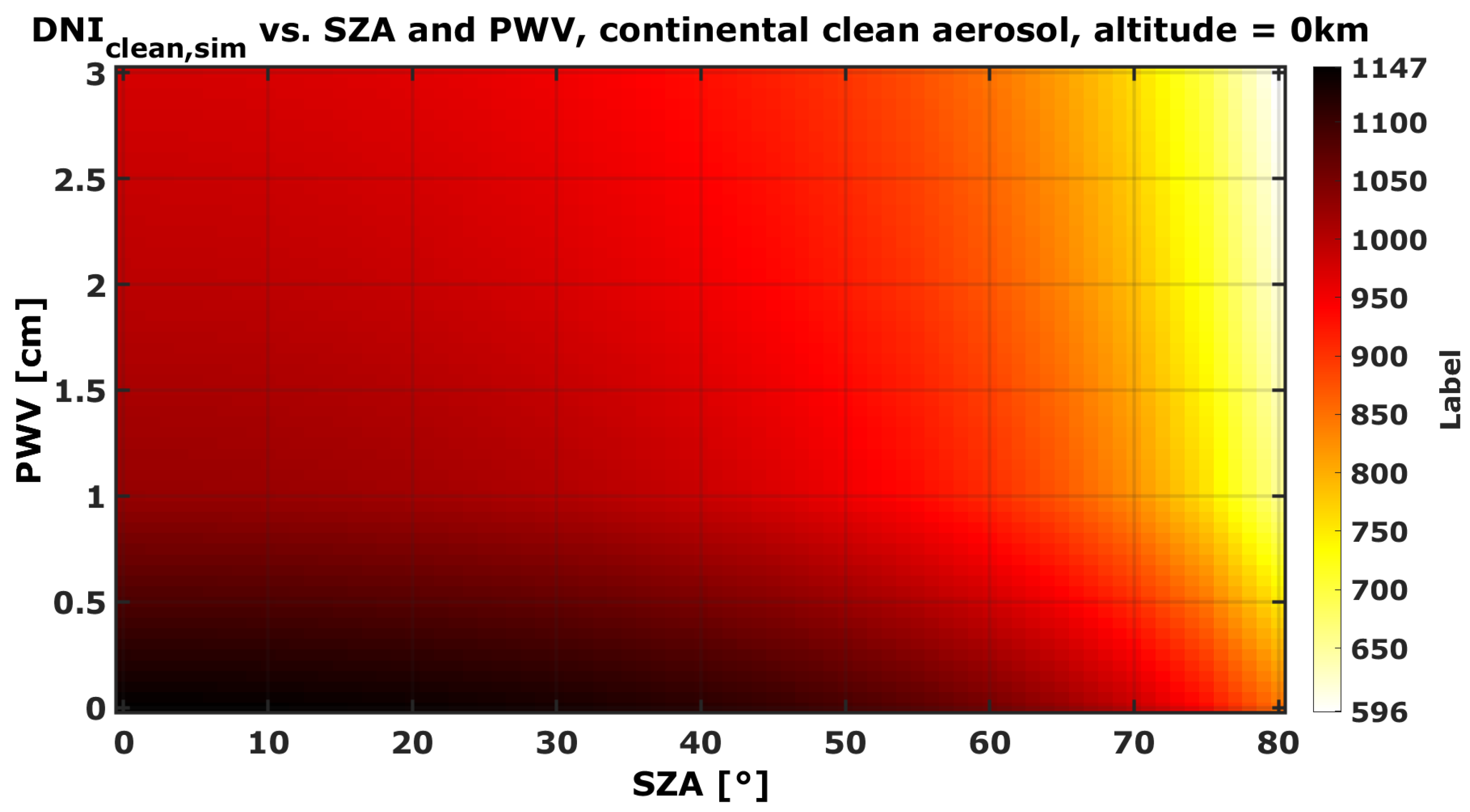
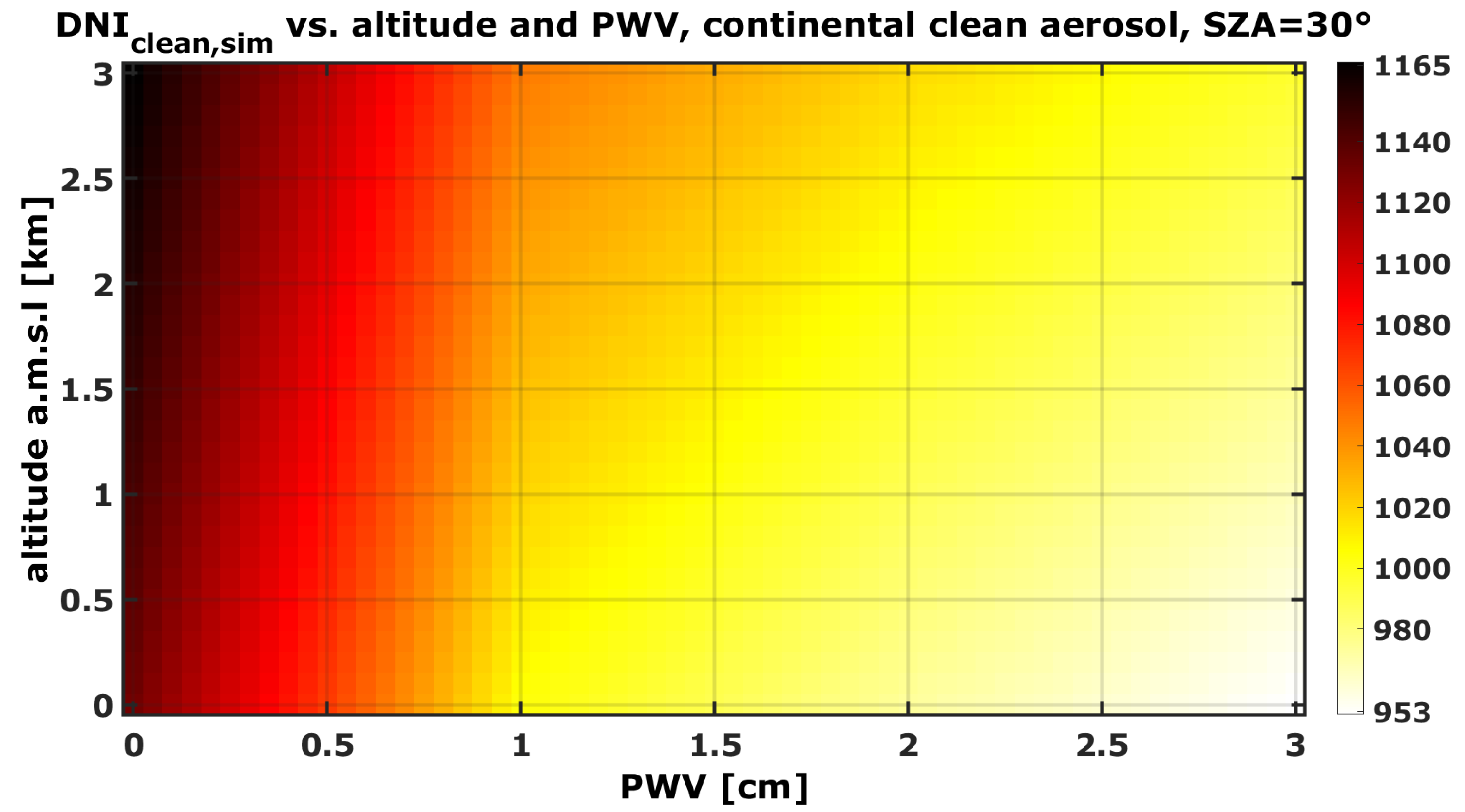
2.2.1. Radiative Transfer Simulations

To enable the application of the developed AATTENUATION model worldwide without the need of further radiative transfer calculations for each site of interest, a LUT was developed. The coefficients a, b and $DN{I}_{clean,sim}$ are stored in the LUT as a function of the SZA, the PWV, the aerosol type and the altitude. According to these parameters for each evaluated time step, the according triplet of the coefficients a and b and $DN{I}_{clean,sim}$ can then be chosen from the LUT.

Radiative transfer calculations with the radiative transfer model libRadtran 2.0-beta [22] were performed for an altitude grid between 0 and 3 km with a resolution of 100 m. The simulations were conducted for a SZA grid between 0 and 80° with 5° resolution and were linearly interpolated for a grid resolution of 1°.

2.2.2. Standard Aerosol Type Mixtures Simulated

The prevailing aerosol type influences the radiative transfer calculations; therefore, the coefficients a and b, LUTs were generated for a variety of standard aerosol types defined in Reference [26]. To facilitate an expert guess of the prevailing aerosol type mixture at the site of interest as described in Section 5, the typical mixtures are briefly described in the following (continental clean, continental average, continental polluted, desert, urban, maritime clean, and maritime tropical).

• Continental aerosol type mixtures: While the continental clean aerosol represents remote continental areas with very low anthropogenic influences and thus no soot contribution to the aerosol mass mixing ratio composition (around 59% water-soluble and 41% insoluble particles), the continental average aerosol describes anthropogenically influenced continental areas with soot and increased insoluble and water-soluble component amounts (58% water-soluble, 40% insoluble particles, and 2% soot mass mixing ratio). The continental polluted standard aerosol is defined by an increased soot mass density and the mass density of water-soluble substances is more than double than in continental average conditions (66% water-soluble, 30% insoluble, and 4% soot in terms of mass mixing ratios).
• Maritime aerosol type mixtures: The maritime aerosol types mainly contain sea salt particles in the coarse and accumulation mode. The maritime clean aerosol represents maritime conditions without soot but some amount of water-soluble aerosol particles to represent non-sea salt sulfate (mass mixing ratios of 91% sea salt of accumulation mode, 1% coarse sea salt, and 7% water-soluble aerosol). In tropical maritime environments, a lower density of water-soluble substances is assumed (93% sea salt in accumulation mode, 1% sea salt in coarse mode, and 6% water-soluble mass mixing ratio).
• Desert aerosol type mixture: The standard desert aerosol composition consists according to Reference [26] of mineral aerosol and water-soluble components (2% water-soluble particles, 3% mineral particles in nucleation, 75% in accumulation, and 20% in coarse mode).
• Urban aerosol type mixture: Strong pollution in urban areas is represented by the urban aerosol mixture (56% water-soluble, 36% insoluble, and 8% soot mass mixing ratio).

2.2.3. Standard Atmospheres and Radiative Transfer Solvers Simulated

The LUTs were generated for both the standard AFGL mid-latitude summer and tropical atmosphere [27]. These standard atmospheres include the profiles of temperature, pressure, air density, water vapor, O${}_2$, O${}_3$, NO${}_2$, and CO${}_2$. The gas absorption parametrization REPTRAN of Reference [28] in medium resolution 5 cm${}^{-1}$ was chosen to parameterize the gas absorption by H${}_2\mathrm{O}$, CO${}_2$, O${}_3$, N${}_2\mathrm{O}$, CO, CH${}_4$, O${}_2$, and N${}_2$. The extraterrestrial solar spectrum source was adopted from Reference [29], and the simulated spectral range was chosen to be 250 nm to 4000 nm with a resolution of 1 nm. As radiative transfer solver, the DISORT model of References [30,31] with 16 streams was selected.

2.2.4. Chosen Extinction Height Profile

For all radiative transfer calculations, an extinction profile with a constant aerosol extinction coefficient up to 1 km above the ground and no extinction above 1 km was considered. In Reference [6], two other options of aerosol extinction profiles were tested for three sites. Although assuming a constant aerosol extinction coefficient up to 1 km above ground performed best for the validation sites in Reference [6], it might be necessary to scale this constant extinction layer thickness according to the site specific conditions, e.g., a constant extinction layer of 500 m or 2 km thickness might fit better for the site of interest. This could be estimated, for example, by considering the average boundary layer height (BLH) from the ERA-Interim reanalysis of ECMWF [32], like tested in Reference [6], for the site of interest. The application of the LUT enables a simple scaling of the resulting extinction coefficient. To scale the extinction coefficient accordingly, a scaling factor of 1/BLH can be simply added to Formula (2) (or to Formula (3), accordingly).

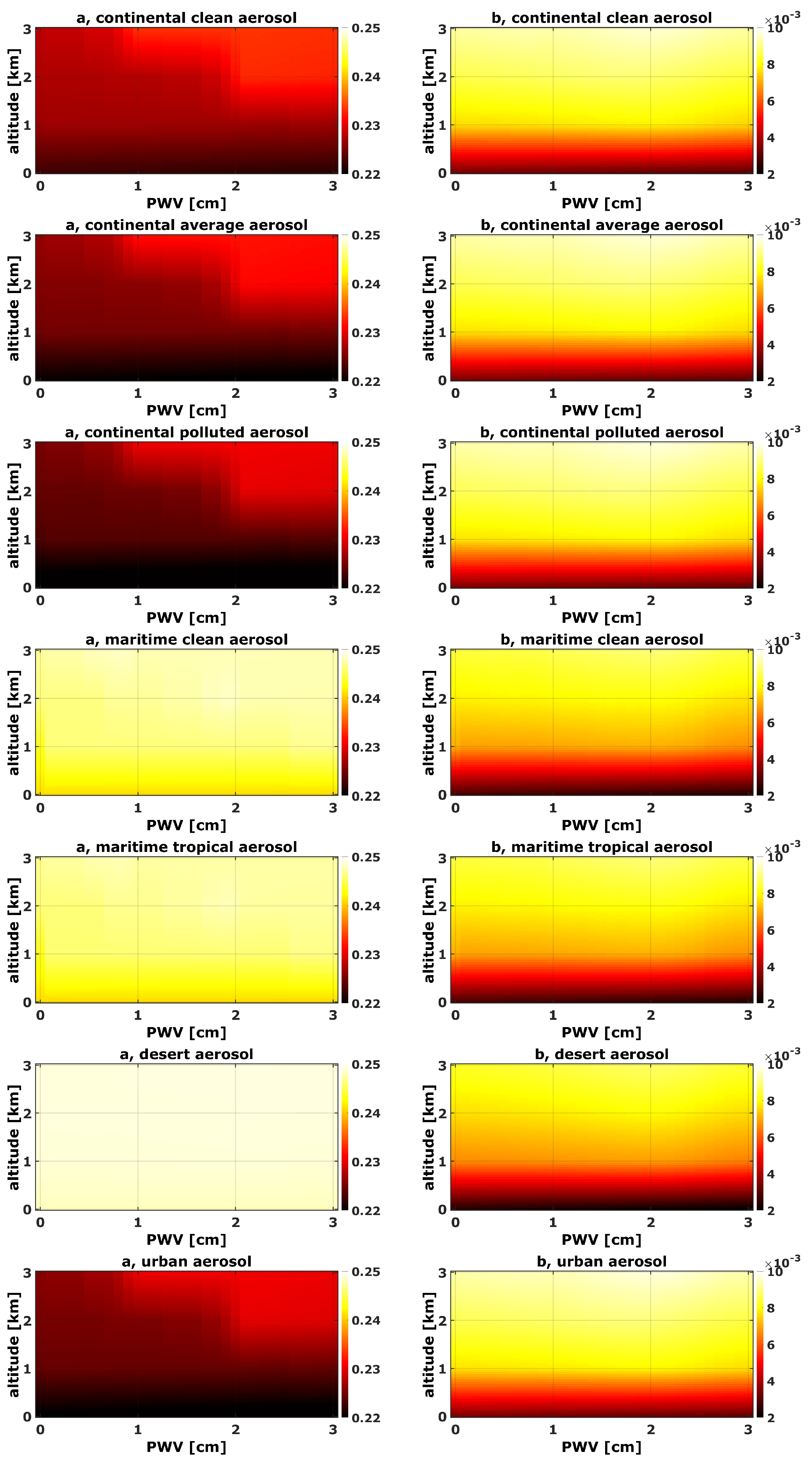
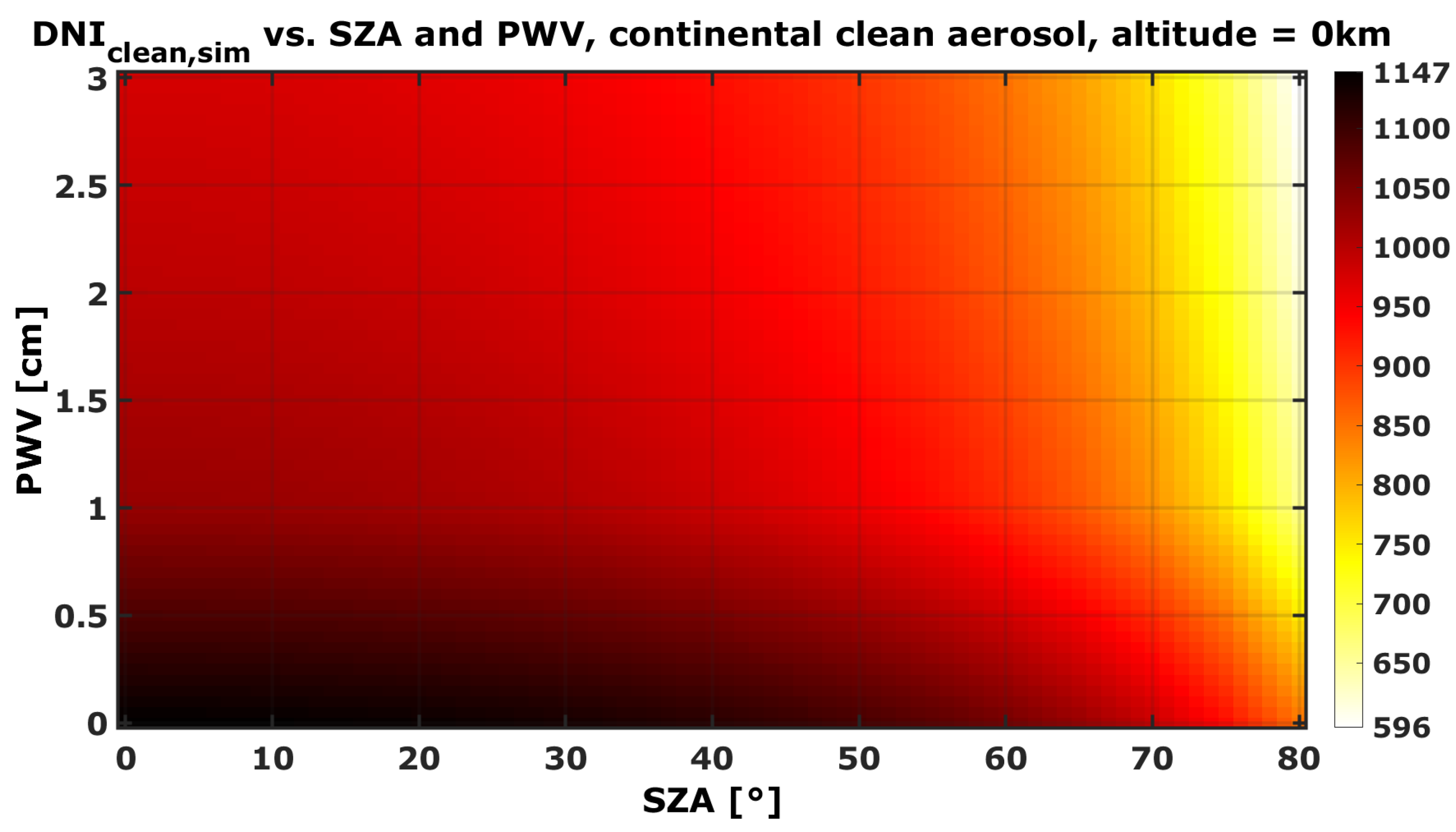
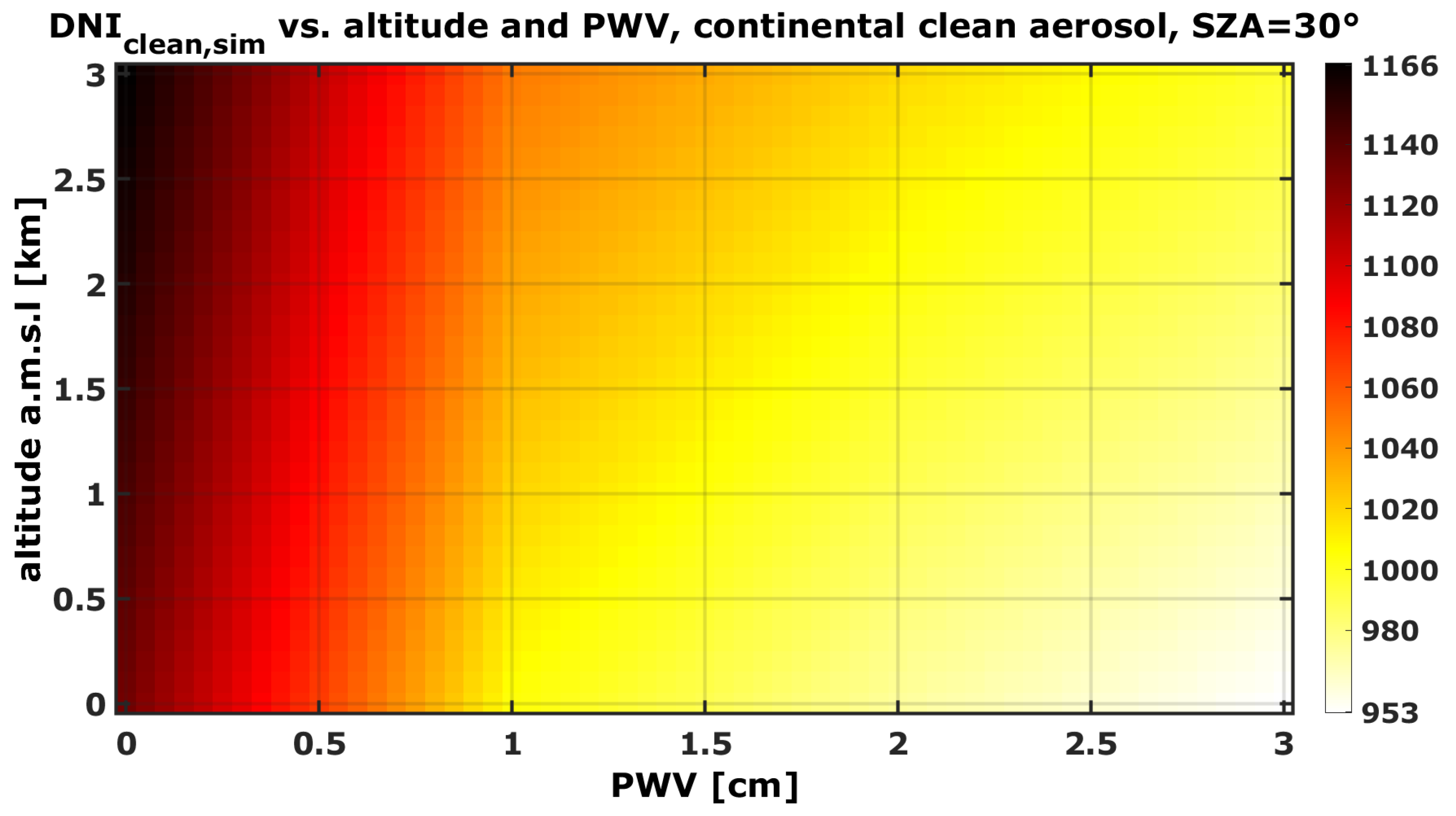
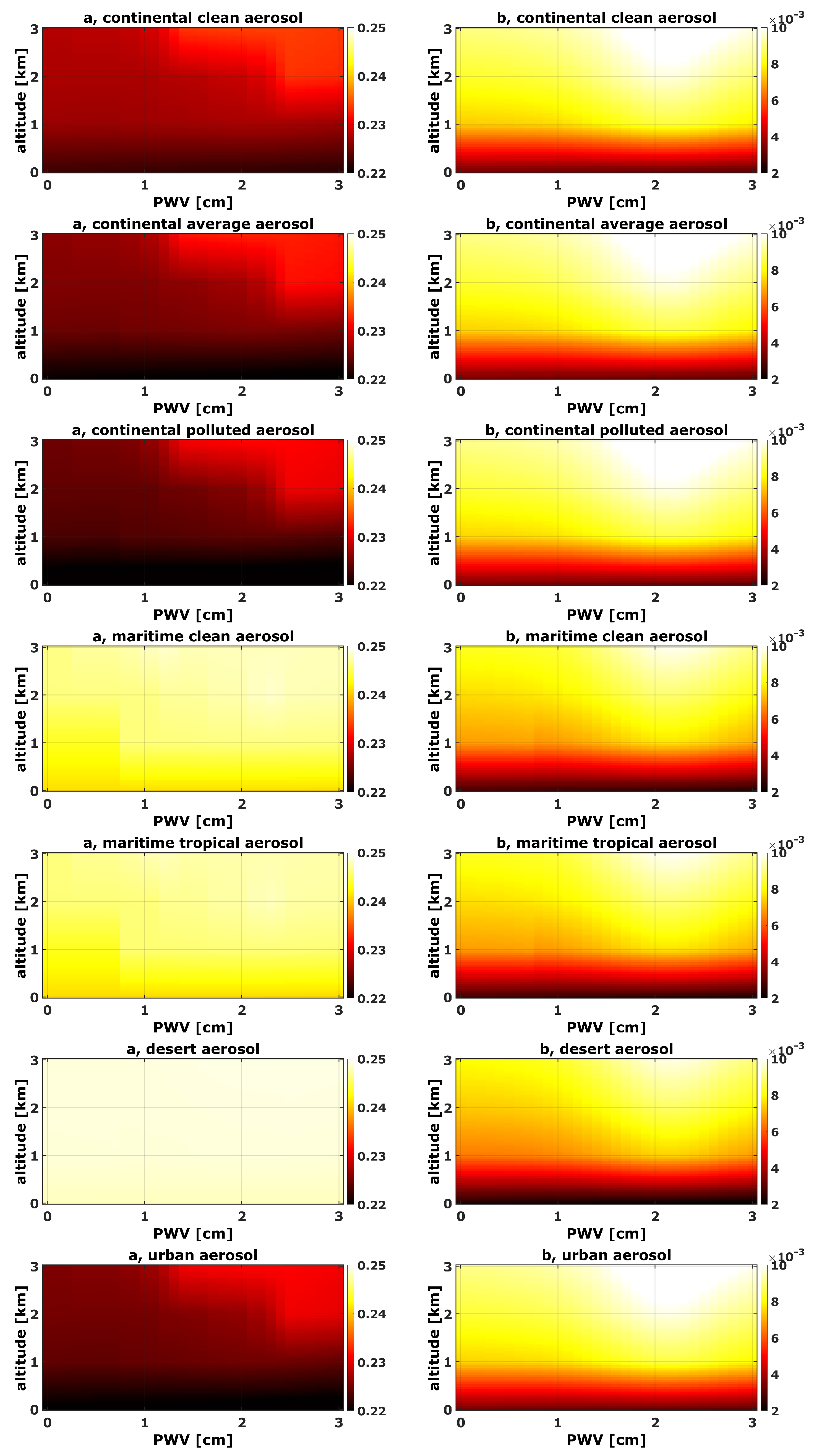
3. AATTENUATION Model Look-Up Table Discussion for Different Aerosol Types

The derived parameters of the LUT which are provided in the supplementary files are analyzed for different aerosol type mixtures and standard atmospheres. The resulting coefficients a and b for the AFGL standard atmosphere for mid-latitudes are shown in Figure 1. It can be seen that, for all typical aerosol type mixtures except for the desert aerosol mixture, a varies with the altitude and is larger for higher altitudes. The PWV level has a stronger influence for the continental average and polluted aerosol than for the continental clean mixture. The parameter a also varies with the PWV level for the urban aerosol mixture.

The parameter b which represents the background extinction level in an atmospheric layer in the absence of aerosol particles (see Equation (2)) is more dependent on the altitude than on the PWV level for all aerosol mixtures. For increasing altitudes, b is also increasing. For the maritime and the desert aerosol mixtures, the change of b with altitude is less pronounced than for the other aerosol mixtures.

The $DN{I}_{clean,sim}$ of the LUT is exemplary displayed for the altitude of 0 km a.m.s.l. (above mean sea level) and dependent on the SZA and PWV in Figure 2. It can be seen that $DN{I}_{clean,sim}$ of the LUT is highest for lowest SZA and PWV levels and increases for higher SZA and PWV levels as expected. In Figure 3, $DN{I}_{clean,sim}$ is shown for a SZA of 30 and an increase of $DN{I}_{clean,sim}$ with the altitude is displayed.

Figure 4, Figure 5 and Figure 6 show the parameters a, b and $DN{I}_{clean,sim}$ of the LUT for the standard AFGL tropical atmosphere. It can be seen that b is stronger influenced by the level of PWV in altitudes above about 1 km. This confirms the presumption mentioned in Reference [21] that the intercept b of Equation (2) varies for the tropics in comparison to the mid-latitudes to accommodate various PWV levels.

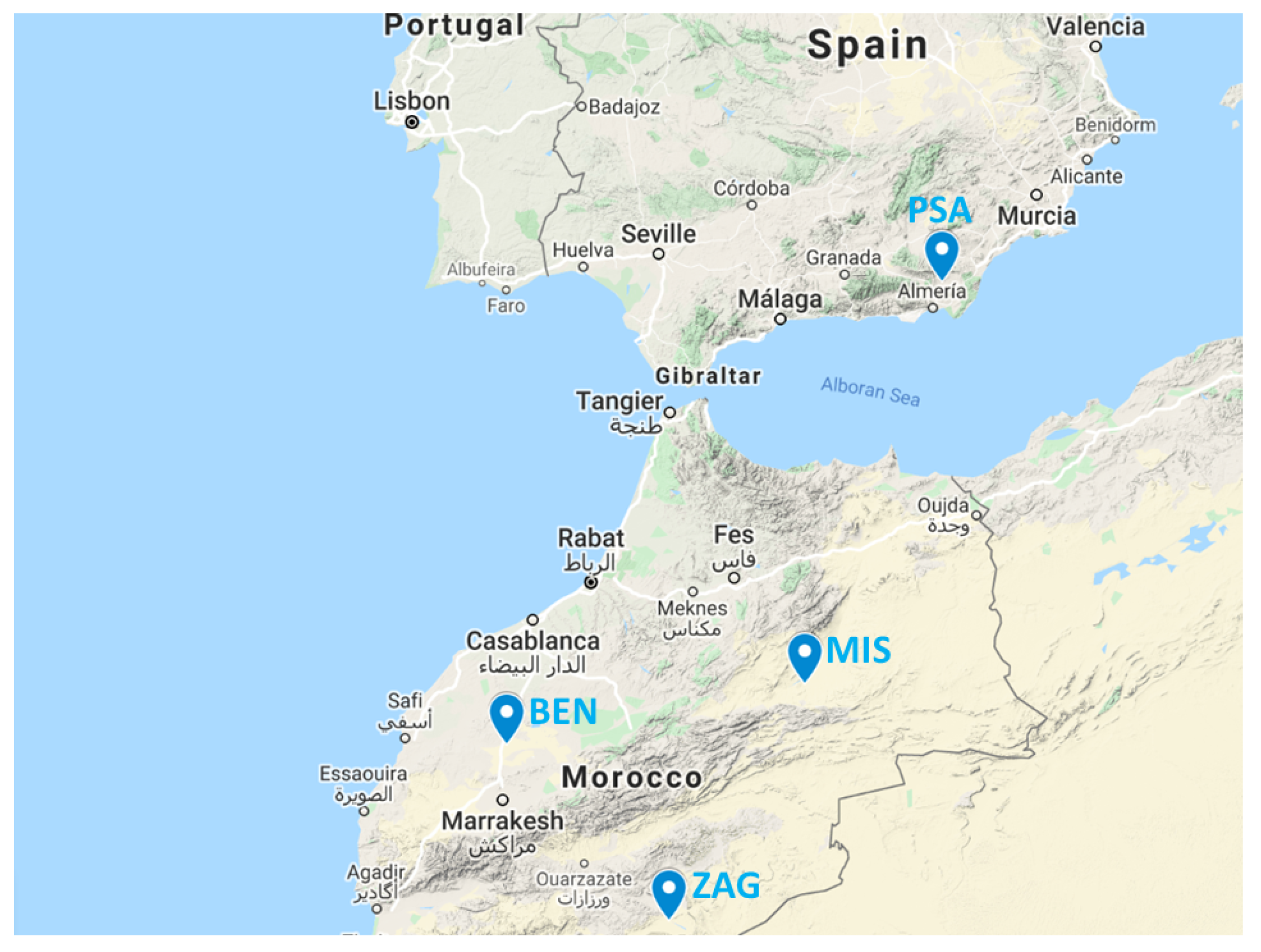
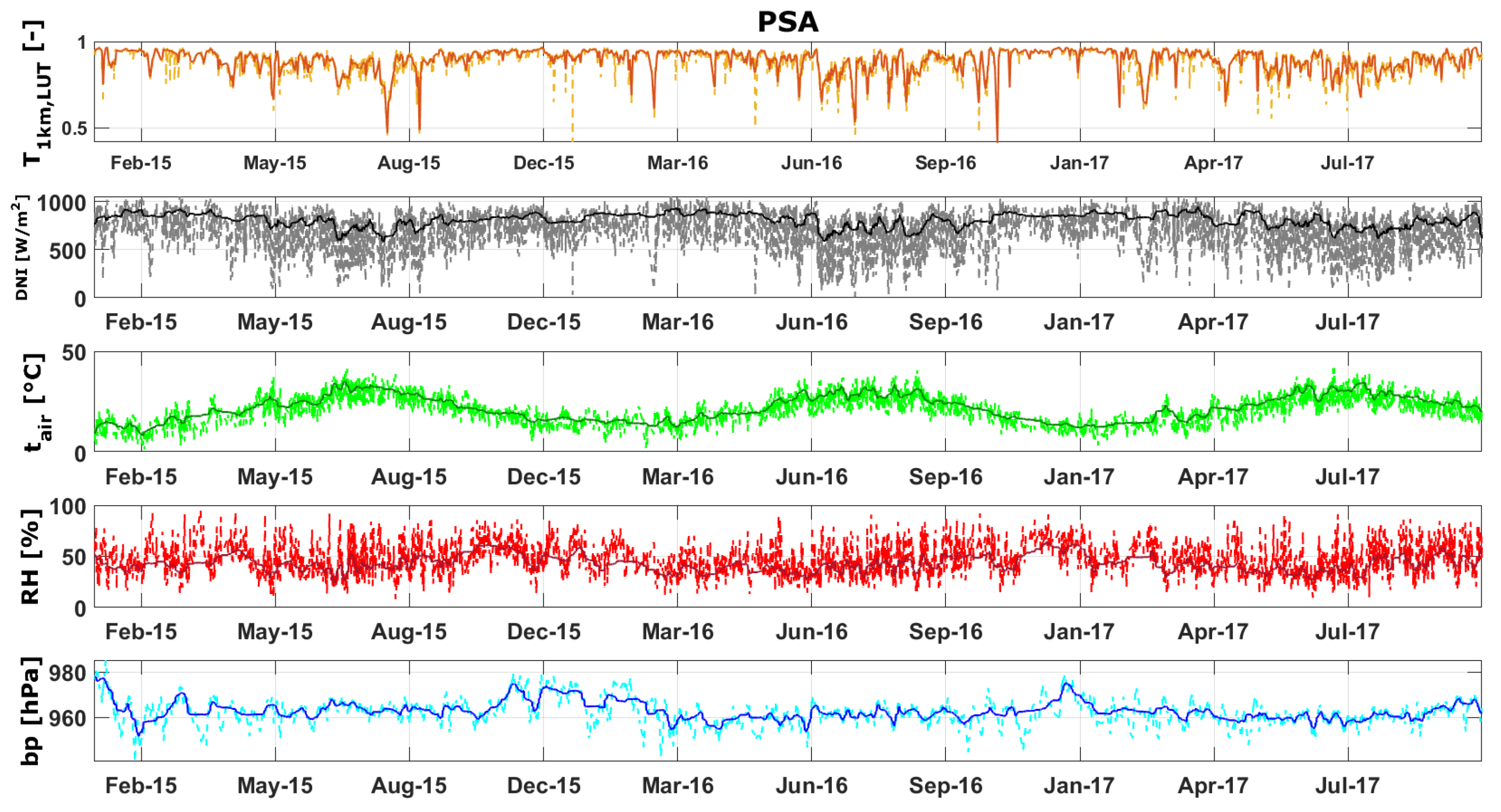
4. AATTENUATION Model Look-Up Table Validation at 4 Sites in Morocco and Spain

The AATTENUATION model including the usage of the LUT was validated at 4 sites in Morocco and Spain (see

Table 1. LibRadtran input for the AATTENUATION model development and LUT.

Site	PSA	MIS	ZAG	BEN
Latitude [° N]	37.091	32.860	30.272	32.22153
Longitude [° E]	−2.358	−4.107	−5.852	−7.92798
Altitude [m a.m.s.l.]	500	1107	783	450
Standard aerosol type	continental	continental	continental	continental
assumed	clean	clean	average	average

) by comparing its results for $T_{1km}$ to the results of the original AATTENUATION model.

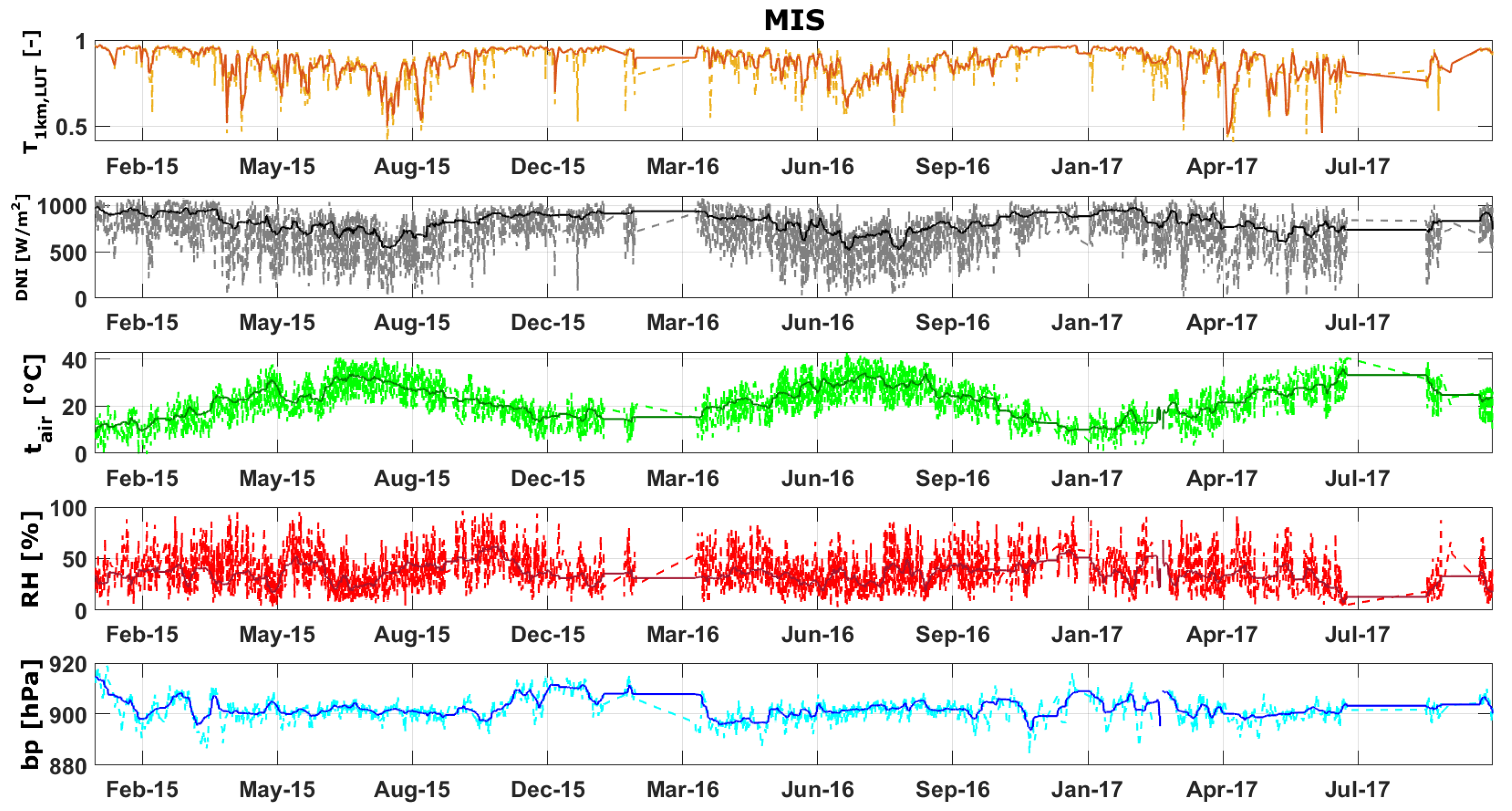
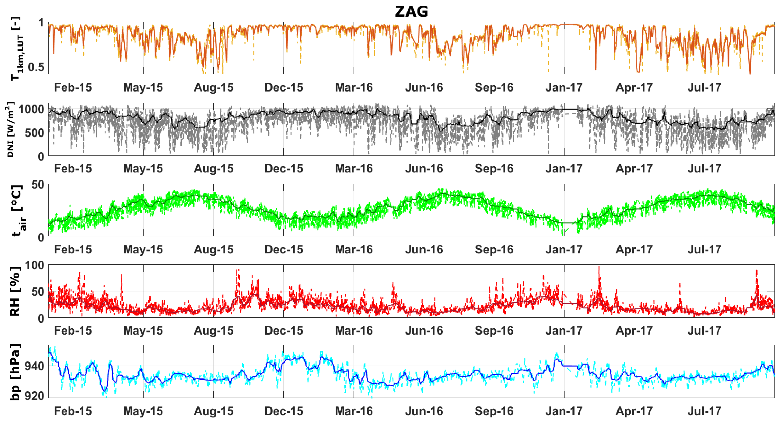
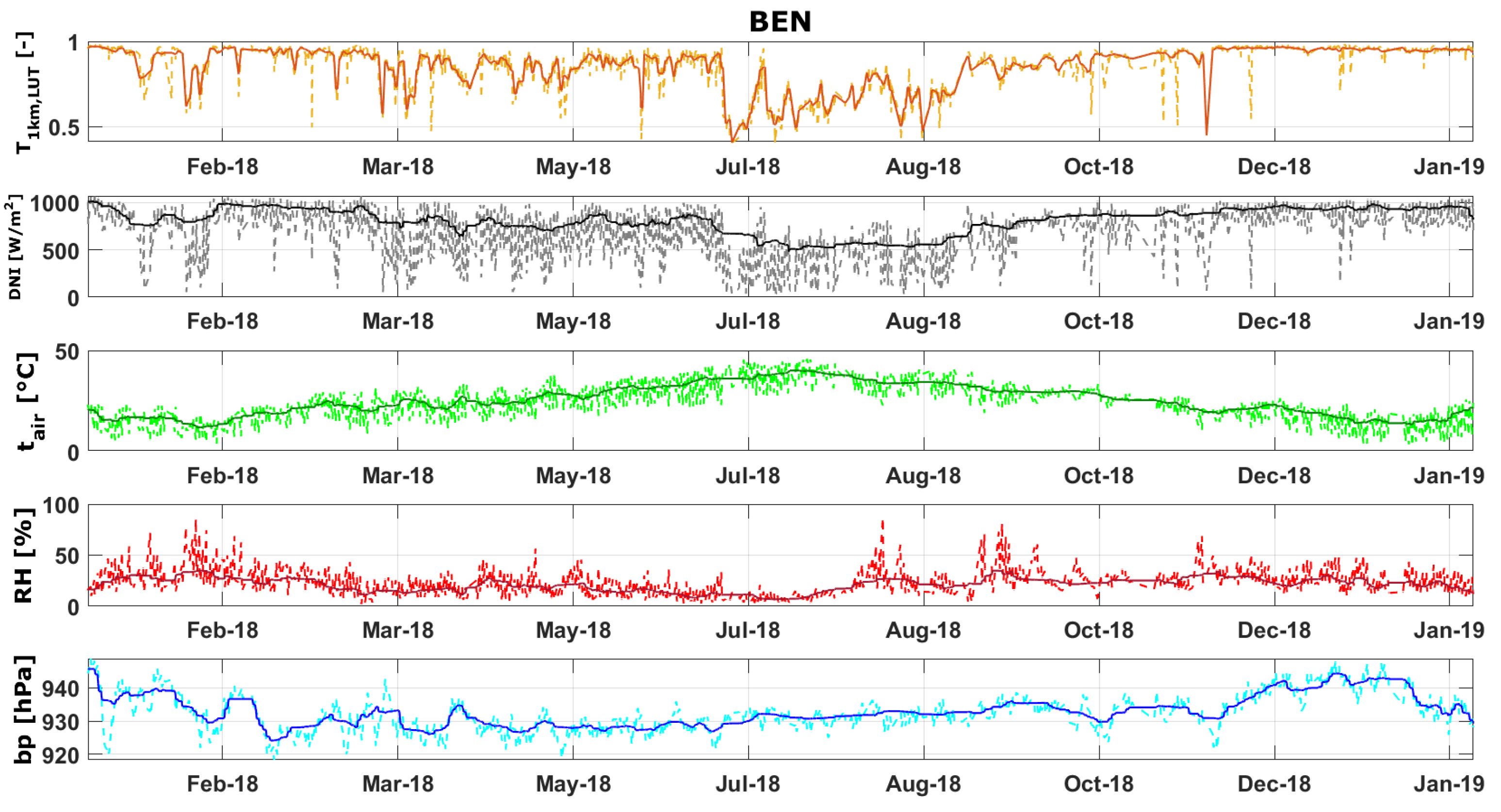
4.1. Reference Data Set

The original AATTENUATION model which was generated for each of the sites individually and which is presented in Reference [19] and validated in Reference [6] is applied by picking the coefficients a, b and $DN{I}_{clean,sim}$ for each time step using on-site data of DNI, temperature, RH and bp at four sites in Southern Spain (CIEMAT’s Plataforma Solar de Almería (PSA)) and Morocco (IRESEN’s stations in Missour, Morocco (MIS), Zagora, Morocco (ZAG), and Benguerir, Morocco (BEN)). This data set serves in this study as reference data set. The generated AATTENUATION model LUT will be validated with this reference data set by choosing the coefficients a, b and $DN{I}_{clean,sim}$ from the LUT for each time step dependent on the same ground based on-site measurements. Figure 7 indicates the location of all investigated sites.

Both the original AATTENUATION model, as well as the AATTENUATION model LUT, are applied only for clear-sky conditions which are detected by using the clear-sky detection described in Section 2. Only clear-sky data points are analyzed in this manuscript because cloudy data points are not relevant for CSP power production, as usually no direct normal radiation is available to be focused by the heliostat field; therefore, also no horizontal attenuation has to be considered for these data points. Therefore, considerations on how to model radiative transfer through cloud fields, e.g., discussed in Reference [33], can be neglected.

At PSA and in MIS, on-site DNI measurements are conducted with a CHP1 pyrheliometer of Reference [34], measured at 1 Hz and saved as 1 min averages. In ZAG, the DNI measurements are performed with a rotating shadowband irradiometer (Twin RSI [35]) and with a temporal resolution of 1 min. For each site, different time periods were selected, for which the $T_{1km}$ which is derived with the AATTENUATION model LUT was compared to the original AATTENUATION model of the according site: At PSA, MIS, and ZAG, all available data between 1 January 2015 and 1 November 2017 were examined. This is the same data set which is shown also in Reference [6]. At BEN, all data points which were available between 1 January 2018 and 1 February 2019 were used for the LUT validation. The corresponding 1-min resolved meteorological ground measurements which were used for the AATTENUATION model are shown in Figure 8, Figure 9, Figure 10 and Figure 11. In the figures, only cloud- and night-filtered data points are shown as described in Section 2. Additionally, a 1-day moving average for the available ground measurements is displayed in the figures. The moving averages can be used to smooth out diurnal noise effects in the ground measurement data and to visualize the dependency of the modeled $T_{1km}$, especially on DNI data.

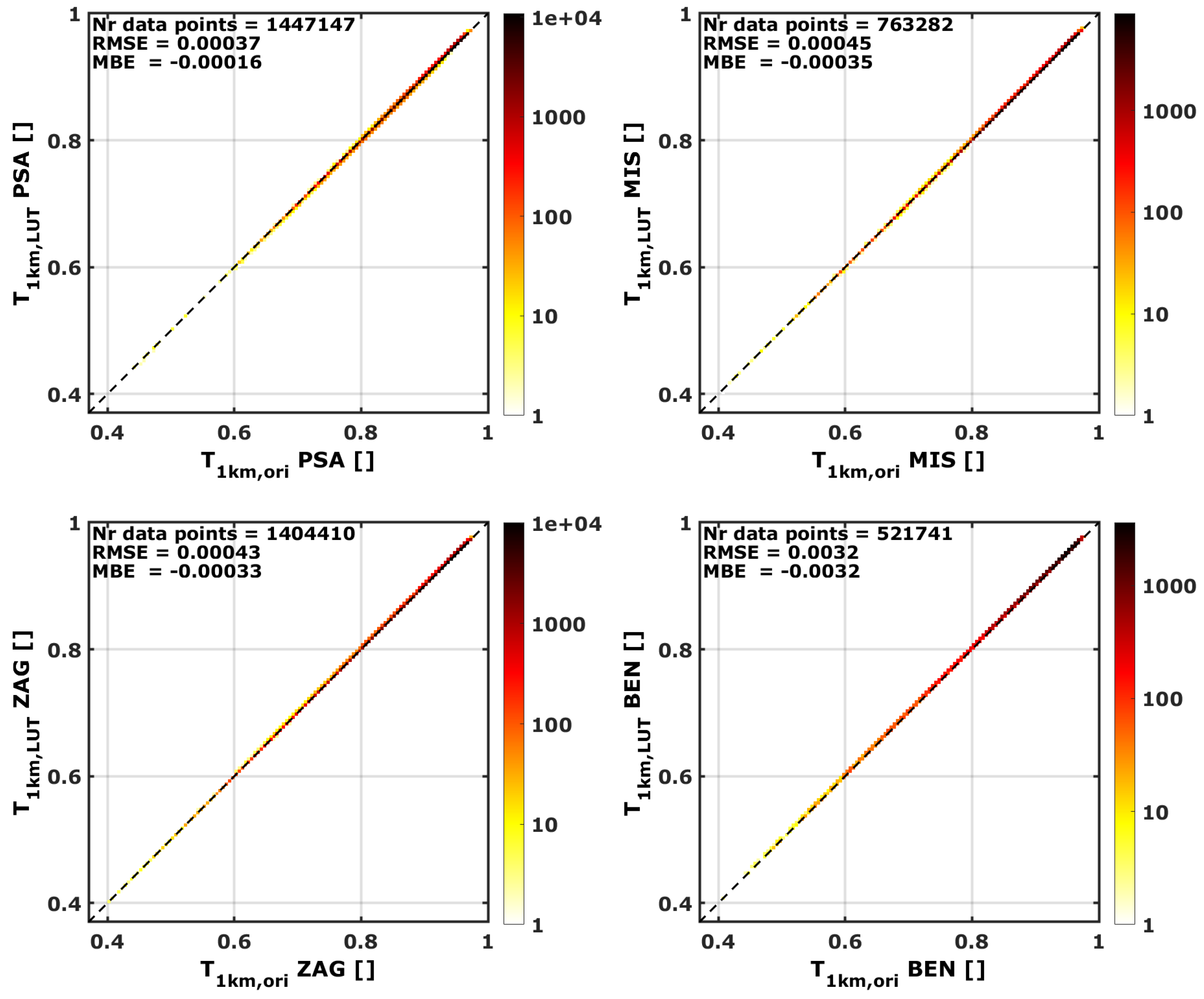
4.2. LUT Validation Results

Figure 12 shows the derived $T_{1km}$ using the original AATTENUATION model in comparison to the $T_{1km}$ derived with the AATTENUATION model LUT for the sites PSA, MIS, ZAG, and BEN. For PSA and MIS, the continental clean aerosol mixture was assumed, while, for ZAG and BEN, the standard continental average mixture was utilized within the applied AATTENUATION model. The color bar and the color distribution in this Figure displays the number of data points per grid point (logarithmic color scale).

It was found that the absolute mean bias error (MBE) or mean bias deviation lies between −0.00016 and −0.00035 of $T_{1km}$ for PSA, MIS, and ZAG. At BEN, the absolute MBE is −0.003. The absolute RMSE for the investigated period 0.00037 and 0.00045 for PSA, MIS, and ZAG and 0.0032 in BEN.

The larger deviations at BEN of almost one decimal place can be explained with the altitude of the site and the resolution of the LUT. The LUT was generated with a resolution of 100 m for the altitude a.m.s.l. When the LUT is applied, the closest altitude grid point within the LUT is chosen. As BEN site altitude of 450 m lies exactly in the center between two LUT grid points, the MBE and RMSE is largest for this site. Additionally, only about half of the number of data points to be examined are available at BEN in comparison to the other sites.

The uncertainty of the original AATTENUATION model is determined in Reference [6] by comparing the derived $T_{1km}$ with on-site transmittance measurements, which were conducted by corrected scatterometer measurements (also see Reference [6,19,36]). It was found that the mean absolute MBE for $T_{1km}$ of the original AATTENUATION model if a constant extinction coefficient in the first kilometer above ground is assumed lies at 0.0033, −0.0011 and −0.0216 for PSA, MIS, and ZAG. The average absolute RMSE was calculated as 0.051, 0.071, and 0.059, respectively.

Therefore, the additional uncertainty which is added by applying the LUT for the AATTENUATION model instead of the original AATTENUATION model is negligible in comparison to the uncertainty derived for the original AATTENUATION model as it is of one magnitude or less smaller.

The largest uncertainty of the AATTENUATION model is caused by the assumption about the extinction profile [6]. The assumption which was used for the creation of the LUT will account only to a certain extent for different sites around the world (depending, for example, of the topography of the site of interest). Therefore, it has to be kept in mind that the AATTENUATION model can be used to estimate the atmospheric attenuation around the world, within its given uncertainty limits.

5. How to Apply the AATTENUATION Model and Its Look-Up Table?

For the usage of the LUT together with the AATTENUATION model, the following steps should be carried out:

• Choose standard atmosphere according to site location: The AATTENUATION model LUT is provided for two different AFGL standard atmosphere files according to Reference [27], which include information about the vertical gas profiles, as well as RH, $T_{air}$, and bp. The LUT is available for the standard mid-latitude summer atmosphere (afglms, to be applied for latitudes until larger than 23° or smaller than −23°) and the AFGL tropical atmosphere for the remaining latitudes in the tropics (afglt, for latitude between −23° and 23°). If you are unsure which atmosphere to use, the model can also be quickly evaluated for both AFGL atmospheres to define a range of possible attenuations. However, the effect of the atmosphere is not significant compared to the aerosol type and model uncertainty.
• Choose prevailing aerosol type according to site location: The LUT is provided for several standard aerosol type mixtures which are defined in Reference [26] and also briefly described in Section 2.2. The LUT is provided for the aerosol type mixture “continental clean”, “continental average”, “continental polluted”, “maritime clean”, “maritime tropical”, “urban”, and “desert”. According to the conditions at the site of interest, one aerosol type mixture can be chosen as an expert guess. Alternatively also several simulations can be carried out to indicate a range of possible attentuations.
• Filter the DNI time series for clouds: A cloud detection algorithm has to be applied to detect cloudy time steps because the AATTENUATION model can only be used for cloud free conditions. An example on how to detect clouds using the TL is described in Reference [19]. The TL coefficient represents the number of dry and clean atmospheres which are producing the observed extinction [37]. To detect cloudy time steps, an upper limit of TL, as well as a limit for the temporal variability of TL, can be defined. In Reference [19], rather conservative cloud detection TL limits were selected for PSA (upper threshold of 13 and temporal variability threshold for 1 min resolved data of 0.02) to avoid outliers which are caused by cloud influenced data points. These thresholds have to be chosen individually for the site of interest.
• Calculate the PWV for time series: For each time step of interest, the PWV within the atmospheric column above the site of interest has to be calculated, e.g., according to the empirical equation of Reference [25]. The equation uses the measured $T_{air}$ and the saturated water vapor pressure which can be calculated from $T_{air}$, RH, and bp using the approach described in Reference [24].
• Find closest altitude grid point for the site of interest: The LUT was created for an altitude grid (a.m.s.l.) with a resolution of 100 m. For the site of interest, the closed altitude grid point has to be found to choose the correct $DN{I}_{clean,sim}$ from the LUT. For higher accuracies of the AATTENUATION model, the $DN{I}_{clean,sim}$ from two grid points can be linearly interpolated according to the actual altitude of the site of interest.
• Consider Earth-Sun distance: As the $DN{I}_{clean,sim}$ from the LUT was simulated and is provided only for 21 June, the effect that the extraterrestrial irradiance varies throughout the year due to the changing sun-earth distance has to be considered. Therefore, the chosen $DN{I}_{clean,sim}$ has to be scaled accordingly. Reference [19] proposes to scale $DN{I}_{clean,sim}$ on a daily basis by calculating the daily squared ratio between the Earth-Sun distance on 21 June ($d_{June21}$) and the actual Earth-Sun distance of the day ($d_i$):

  $$rati{o}_{earth,sun}={\left({\displaystyle \frac{d_{June21}}{d_i}}\right)}^2.$$

  (4)
  The $DN{I}_{clean,sim}$ from the LUT is than multiplied by this ratio. These daily ratios, which were calculated according to Reference [38], are provided with the LUT.
• Calculate the SZA for each time step: The SZA has to be calculated for the whole time series because, according to the time-dependent SZA, $DN{I}_{clean,sim}$ has to be chosen to be used in Equation (3). This can be done by, e.g., applying the Michalsky code [39] and NREL’s SOLPOS code (https://www.nrel.gov/grid/solar-resource/solpos.html), which was done for the evaluation presented in this manuscript, or, e.g., the solar position code of Reference [40] can be used.
• Choose AATTENUATION model LUT parameters for each time step: For each time step from the time series of interest, the parameters a, b and $DN{I}_{clean,sim}$ can now be chosen from the LUT according to the current PWV, SZA, the site altitude and the assumed prevailing aerosol type. These parameters can then be applied in Equation (3) to calculate the time-dependent attenuation or transmittance dependent on the slant range.
• Scale the extinction coefficient: If no further adjustments are made, an extinction profile with a constant aerosol extinction coefficient up to 1 km above the ground and no extinction above 1 km will be assumed. If necessary, this constant extinction layer thickness can be scaled now according to the site specific conditions, e.g., by considering the BLH from other sources. To scale the extinction coefficient, a scaling factor of 1/BLH can be added to Formula (2).
• Extent attenuation simulations to SZA larger than 80°: The AATTENUATION LUT is provided only for SZA of less than 80°. The DNI curve is for cloud free days rather steep between 80 and 90° and small measurement errors in DNI will have a large impact on the modeled attenuation than for lower SZA. Therefore, no LUT is provided for these high SZA. Different strategies can be followed to approximate the attenuation for the time steps with SZA between 80° and 90° when a small part of solar radiation is still available. For the LUT generation, this effect was neglected as these SZAs are of low importance for CSP yield calculations. The recommended strategy to derive attenuation simulations for SZA between 80° and 90° is to use the last simulated attenuation value of each day for the time steps between SZA equal to 80° and 90° in the afternoon. In the morning, the first calculated attenuation value can be applied for all previous data point of SZA between 80° and 90°.

6. Conclusions

An AATTENUATION model developed in References [19,21,41,42] was validated at three sites in Reference [6]. With this model, the atmospheric attenuation in solar tower plants can be estimated site-dependently. The model is only dependent on DNI, $T_{air}$, RH, and bp data sets, which are usually available at sites of interest during the site assessment phase.

A new LUT for the AATTENUATION model is presented in this manuscript. The LUT enables a simple and worldwide applicability of the model and the according LUT data are published as supplementary files with this manuscript. With the help of this LUT, the time-consuming radiative transfer calculations which had to be performed in the past for each site of interest can be avoided. For a simple application, a step-by-step description on how to use the AATTENUATION model and the LUT at the site of interest is given.

The LUT was developed for 7 typical aerosol type mixtures from the Optical Properties of Aerosols and Clouds (OPAC) library of Reference [26] (continental clean, continental average, continental polluted, maritime clean, maritime tropics, desert, and urban) which main components are summarized in this manuscript. Further, the parameters covered by the LUT are provided for two standard atmospheres defined by Reference [27] (AFGL for mid-latitudes and for the tropics).

The usage of the new introduced LUT does not increase the uncertainties of the AATTENUATION model in a noticeable way. This was found by comparing the results of the original AATTENUATION model with the AATTENUATION model using the LUT at four sites in Morocco and Spain.

These new developments facilitate the estimation of atmospheric attenuation levels in solar CSP tower plants site- and time-dependent. The AATTENUATION model and the according LUT can be applied to retrieve information if atmospheric attenuation is an issue for the site of interest. If it is not clear which aerosol type mixture is typical for the site of interest, the model can be applied several times for different aerosol types to retrieve information about the possible extinction range. The same accounts for the assumed vertical profile of the extinction, which can be scaled dependent on the presumed thickness of the aerosol layer above ground. Here, a homogeneous extinction layer of 1 km thickness was assumed, but estimation of the possible range of the attenuation, e.g., thicknesses of 500 m or 2 km, can be calculated, as well. If the results for the site show high attenuation levels, further on-site measurements of the extinction coefficient are recommended.

References

1. Washington, R.; Todd, M.; Middleton, N.; Goudie, A.S. Dust-Storm Source Areas Determined by the Total Ozone Monitoring Spectrometer and Surface Observations. Ann. Assoc. Am. Geogr. 2003, 93, 297–313. [Google Scholar] [CrossRef]
2. Abengoa. 2015. Available online: http://www.abengoasolar.com (accessed on 15 January 2015).
3. Torresol. 2015. Available online: http://www.torresolenergy.com (accessed on 15 January 2015).
4. Brightsource. 2015. Available online: http://www.ivanpahsolar.com/ (accessed on 15 January 2015).
5. Hanrieder, N.; Wilbert, S.; Mancera Guevara, D.; Buck, R.; Giuliano, S.; Pitz-Paal, R. Atmospheric extinction in solar tower plants—A Review. Sol. Energy 2017, 152, 193–207. [Google Scholar] [CrossRef]
6. Hanrieder, N.; Ghennioui, A.; Alami Merrouni, A.; Wilbert, S.; Wiesinger, F.; Sengupta, M.; Zarzalejo, L.; Schade, A. Atmospheric Transmittance Model Validation for CSP Tower Plants. Remote Sens. 2019, 11, 1083. [Google Scholar] [CrossRef] [Green Version]
7. IRENA. International Renewable Energy Agency, Africa 2030: Roadmap for a Renewable Energy Future; Report; IRENA: Abu Dhabi, UAE, 2015. [Google Scholar]
8. Polo, J.; Ballestrín, J.; Carra, E. Sensitivity study for modelling atmospheric attenuation of solar radiation with radiative transfer models and the impact in solar tower plant production. Sol. Energy 2016, 134, 219–227. [Google Scholar] [CrossRef]
9. Polo, J.; Ballestrín, J.; Alonso-Montesinos, J.; López-Rodriguez, G.; Barbero, F.; Carra, E.; Fernández-Reche, J.; Bosch, J.; Batlles, F. Analysis of solar tower plant performance influenced by atmospheric attenuation at different temporal resolutions related to aerosol optical depth. Sol. Energy 2018, 157. [Google Scholar] [CrossRef]
10. Armijo, K.; Shinde, S. Heat Transfer Phenomena in Concentrating Solar Power Systems; SAND2016-11399; Sandia National Lab. (SNL-NM): Albuquerque, NM, USA, 2016. [CrossRef]
11. Tasbirul Islam, M.; Huda, N.; Abdullah, A.; Saidur, R. A comprehensive review of state-of-the-art concentrating solar power (CSP) technologies: Current status and research trends. Renew. Sustain. Energy Rev. 2018, 91, 987–1018. [Google Scholar] [CrossRef]
12. Elias, T.; Ramon, D.; Garnero, M.A.; Dubus, L.; Bourdil, C. Solar Energy Incident at the Receiver of a Solar Tower Plant, Derived from Remote Sensing: Computation of Both DNI and Slant Path Transmittance. In AIP Conference Proceedings; AIP Publishing LLC: Melville, NY, USA, 2017. [Google Scholar]
13. Elias, T.; Ramon, D.; Brau, J.; Moulana, M. Sensitivity of the Solar Resource in Solar Tower Plants to Aerosols and Water Vapor. In AIP Conference Proceedings; AIP Publishing LLC: Melville, NY, USA, 2018. [Google Scholar]
14. Lopez, G.; Gueymard, C.; Bosch, J.L. Evaluation of Solar Energy Losses for the Heliostat-To-Receiver Path of a Tower Solar Plant for Different Aerosol Models; Solar World Congress: Abu Dhabi, UAE, 2017. [Google Scholar]
15. Lopez, G.; Gueymard, C.; Bosch, J.L.; Rapp-Arraras, I.; Alonso-Montesinos, J.; Pulido-Calvo, I.; Ballestrín, J.; Polo, J.; Barbero, J. Modeling Water Vapor Impact on the Solar Energy Reaching the Receiver of a Solar Tower Plant by means of Artificial Neural Networks. Sol. Energy 2018, 169, 34–39. [Google Scholar] [CrossRef]
16. Gueymard, C.; Lopez, G.; Rapp-Arraras, I. Atmospheric Transmission Loss in Mirror-To-Tower Slant Ranges Due to Water Vapor. In AIP Conference Proceedings; AIP Publishing LLC: Melville, NY, USA, 2017. [Google Scholar]
17. Carra, E.; Ballestrín, J.; Polo, J.; Barbero, F.; Fernández-Reche, J. Atmospheric extinction levels of solar radiation at Plataforma Solar de Almería. Application to solar thermal electric plants. Energy 2018, 145, 400–407. [Google Scholar] [CrossRef]
18. Polo, J.; Alonso-Montesinos, J.; López-Rodriguez, G.; Bosch, J.; Barbero, F.; Carra, E.; Fernández-Reche, J.; Batlles, F.; Ballestrín, J. Modelling atmospheric attenuation at different AOD time-scales in yield performance of solar tower plants. In AIP Conference Proceedings; AIP Publishing LLC: Melville, NY, USA, 2018; Volume 2033, p. 190013. [Google Scholar] [CrossRef]
19. Hanrieder, N.; Sengupta, M.; Xie, Y.; Wilbert, S.; Pitz-Paal, R. Modelling Beam Attenuation in Solar Tower Plants Using Common DNI Measurements. Sol. Energy 2016, 129, 244–255. [Google Scholar] [CrossRef]
20. Vindel, J.; Polo, J.; Zarzalejo, L.; Ramirez, L. Stochastic model to describe atmospheric attenuation from yearly global solar irradiation. Atmos. Res. 2015, 153, 205–216. [Google Scholar] [CrossRef]
21. Sengupta, M.; Wagner, M. Impact of Aerosols on Atmospheric Attenuation Loss in Central Receiver Systems. In AIP Conference Proceedings; AIP Publishing LLC: Melville, NY, USA, 2012. [Google Scholar]
22. Mayer, B.; Kylling, A. Technical note: The libRadtran software package for radiative transfer calculations-description and example of use. Atmos. Chem. Phys. 2005, 5, 1855–1877. [Google Scholar] [CrossRef] [Green Version]
23. Emde, C.; Buras-Schnell, R.; Kylling, A.; Mayer, B.; Gasteiger, J.; Hamann, U.; Kylling, J.; Richter, B.; Pause, C.; Dowling, T.; et al. The libRadtran software package for radiative transfer calculations (version 2.0.1). Geosci. Model Dev. 2016, 9, 1647–1672. [Google Scholar] [CrossRef] [Green Version]
24. Gueymard, C. Assessment of the Accuracy and Cumputing Speed of Simplified Saturation Vapor Equations Using a New Reference Dataset. J. Appl. Meteorol. 1993, 32, 1294–1300. [Google Scholar] [CrossRef] [Green Version]
25. Gueymard, C. Analysis of monthly average atmospheric precipitable water and turbidity in Canada and Northern United States. Sol. Energy 1994, 53, 57–71. [Google Scholar] [CrossRef]
26. Hess, M.; Köpke, P.; Schult, I. Optical Properties of Aerosols and Clouds: The Software Package OPAC. Bull. Am. Soc. 1998, 79, 831–844. [Google Scholar] [CrossRef]
27. Anderson, G.; Clough, S.; Kneizys, F.X.; Chetwynd, J.; Shettle, E. AFGL Atmospheric Constituent Profiles (1–120 km); Environmental Research Papers; AFGL-TR-89-0110; Air Force Geophysics Laboratory: Bedford, MA, USA, 1986; Volume 954. [Google Scholar]
28. Gasteiger, J.; Emde, C.; Mayer, B.; Buras, R.; Buehler, S.; Lemke, O. Representative wavelengths absorption parametrization applied to satellite channels and spectral bands. J. Quant. Spectrosc. Radiat. Transf. 2014, 148, 99–115. [Google Scholar] [CrossRef]
29. Kurucz, R. Synthetic infrared spectra. In Proceedings of the 154th Symposium of the International Astronomical Union (IAU), Tucson, AZ, USA, 2–5 March 1992; Kluwer, Acad.: Norwell, MA, USA, 1992. [Google Scholar]
30. Stamnes, K.; Tsay, S.; Wiscombe, W.; Jayaweera, K. Numerically stable algorithm for discrete-ordinate-method radiative transfer in multiple scattering and emitting layered media. Appl. Opt. 1988, 27, 2502–2509. [Google Scholar] [CrossRef]
31. Buras, R.; Dowling, T.; Emde, C. New secondary-scattering correction in DISORT with increased efficiency for forward scattering. J. Quant. Spectrosc. Radiat. Transf. 2011, 112, 2028–2034. [Google Scholar] [CrossRef]
32. Berrisford, P.; Dee, D.; Poli, P.; Brugge, R.; Fielding, K.; Fuentes, M.; Kallberg, P.; Kobayashi, S.; Uppala, S.; Simmons, A. The ERA-Interim archive Version 2.0; Report; ECMWF: Reading, UK, 2011. [Google Scholar]
33. Lane-Veron, D.; Somerville, C.J. Stochastic theory of radiative transfer through generalized cloud fields. J. Geophys. Res. 2004, 109, D18113. [Google Scholar] [CrossRef]
34. Kipp and Zonen. CHP1 Pyrheliometer Instruction Manual (Version 0811); KippZonen: Utrecht, The Netherlands, 2008. [Google Scholar]
35. CSPServices. Twin RSI Description. 2020. Available online: https://www.cspservices.de/wp-content/uploads/Folleto_Twin_RSI.pdf (accessed on 17 July 2020).
36. Hanrieder, N.; Wilbert, S.; Pitz-Paal, R.; Emde, C.; Gasteiger, J.; Mayer, B.; Polo, J. Atmospheric extinction in solar tower plants: Absorption and broadband correction for MOR measurements. Atmos. Meas. Tech. 2015, 8, 1–14. [Google Scholar] [CrossRef] [Green Version]
37. Ineichen, P.; Perez, R. A new airmass indepentend formulation for the Linke turbidity coefficient. Sol. Energy 2002, 73, 151–157. [Google Scholar] [CrossRef] [Green Version]
38. Liou, K. An Introduction to Atmospheric Radiation, 2nd ed.; International Geophysics Series; Academic Press: London, UK, 2002; Volume 84. [Google Scholar]
39. Michalsky, J. The Astronomical Almanac’s algorithm for approximate solar position (1950–2050). Sol. Energy 1988, 40, 227–235, Erratum in 1988, 41, 113. [Google Scholar] [CrossRef]
40. Blanc, P.; Wald, L. The SG2 algorithm for a fast and accurate computation of the position of the Sun for multi-decadal time period. Sol. Energy 2012, 86, 3072–3083. [Google Scholar] [CrossRef] [Green Version]
41. Sengupta, M.; Wagner, M. Estimating atmospheric attenuation in central receiver systems. In Proceedings of the ASME 2012 6th International Conference on Energy Sustainability, San Diego, CA, USA, 23–26 July 2012. [Google Scholar]
42. Sengupta, M.; Wagner, M. Atmospheric Attenuation in Central Receiver Systems from DNI Measurements. In AIP Conference Proceedings; AIP Publishing LLC: Melville, NY, USA, 2013. [Google Scholar]
Figure 1. Look-up table (LUT) coefficients a and b for different standard aerosol types dependent on the altitude above mean sea level (a.m.s.l.) and the precipitable water vapor (PWV) for the standard AFGL atmosphere for mid-latitudes (afglms). The LUTs are provided together with this manuscript as supplementary files.
Energies 13 05248 g001
Figure 2. LUT direct normal irradiance ( D N I ) c l e a n , s i m for an atmosphere without aerosol particles dependent on the standard visual range (SZA) and the PWV for the standard AFGL atmosphere for mid-latitudes (afglms) for the altitude equal 0 km a.m.s.l. The LUT D N I c l e a n , s i m is provided within the supplementary files.
Energies 13 05248 g002
Figure 3. LUT D N I c l e a n , s i m for an atmosphere without aerosol particles dependent on the altitude a.m.s.l. and the PWV for the standard AFGL atmosphere for mid-latitudes (afglms) for the SZA equal 30°. The LUT D N I c l e a n , s i m is provided within the supplementary files.
Energies 13 05248 g003
Figure 4. LUT coefficients a and b for different standard aerosol types dependent on the altitude a.m.s.l. and the PWV for the standard AFGL atmosphere for the tropics (afglt). The LUTs are provided together with this manuscript as supplementary files.
Energies 13 05248 g004
Figure 5. LUT D N I c l e a n , s i m for an atmosphere without aerosol particles dependent on the SZA and the PWV for the standard AFGL atmosphere for the tropics (afglt) for the altitude equal 0 km a.m.s.l. The LUT D N I c l e a n , s i m is provided within the supplementary files.
Energies 13 05248 g005
Figure 6. LUT D N I c l e a n , s i m for an atmosphere without aerosol particles dependent on the altitude a.m.s.l. and the PWV for the standard AFGL atmosphere for the tropics (afglt) for the SZA equal 30°. The LUT D N I c l e a n , s i m is provided within the supplementary files.
Energies 13 05248 g006
Figure 7. Investigated locations of Plataforma Solar de Almería (PSA), Missour, Morocco (MIS), Zagora, Morocco (ZAG), and Benguerir, Morocco (BEN). Source: Google.
Energies 13 05248 g007
Figure 8. One-minute resolved meteorological ground measurements of broadband transmittance for a slant range of 1 km ( T 1 k m ), DNI, ambient temperature ( T a i r ), relative humidity (RH), and barometric pressure (bp) at PSA between January 2015 and October 2017. Only cloud- and night-filtered data points are shown. One-minute resolved data are displayed with a broken line; 1-day moving averages with a solid line.
Energies 13 05248 g008
Figure 9. One-minute resolved meteorological ground measurements of T 1 k m , DNI, T a i r , RH, and bp at MIS between January 2015 and October 2017. Only cloud- and night-filtered data points are shown. One-minute resolved data are displayed with a broken line; 1-day moving averages with a solid line.
Energies 13 05248 g009
Figure 10. One-minute resolved meteorological ground measurements of T 1 k m , DNI, T a i r , RH, and bp at ZAG between January 2015 and October 2017. Only cloud- and night-filtered data points are shown. One-minute resolved data are displayed with a broken line; 1-day moving averages with a solid line.
Energies 13 05248 g010
Figure 11. One-minute resolved meteorological ground measurements of T 1 k m , DNI, T a i r , RH, and bp at BEN between January 2018 and January 2019. Only cloud- and night-filtered data points are shown. One-minute resolved data are displayed with a broken line; 1-day moving averages with a solid line.
Energies 13 05248 g011
Figure 12. Derived T 1 k m with the original AATTENUATION model radiative transfer calculations versus with the LUT coefficients for the AATTENUATION model for four sites PSA, MIS, ZAG, and BEN. The color bar displays the number of data points per grid point (logarithmic color scale).
Energies 13 05248 g012