Article

Research on Fault Detection for Three Types of Wind Turbine Subsystems Using Machine Learning

1
School of Control Science and Engineering, Hebei University of Technology, Tianjin 300131, China
2
School of Electronic and Control Engineering, North China Institute of Aerospace Engineering, Langfang 065000, China
3
Faculty of Engineering and Information Sciences, University of Wollongong, Wollongong, NSW 2522, Australia
4
Department of Technical Development, AT&M Environmental Engineering Technology Co., Ltd., Beijing 100801, China
*
Author to whom correspondence should be addressed.
Energies 2020, 13(2), 460; https://doi.org/10.3390/en13020460
Submission received: 19 October 2019 / Revised: 12 January 2020 / Accepted: 14 January 2020 / Published: 17 January 2020
(This article belongs to the Section A3: Wind, Wave and Tidal Energy)

Abstract

:
In wind power generation, one aim of wind turbine control is to maintain it in a safe operational status while achieving cost-effective operation. The purpose of this paper is to investigate new techniques for wind turbine fault detection based on supervisory control and data acquisition (SCADA) system data in order to avoid unscheduled shutdowns. The proposed method starts with analyzing and determining the fault indicators corresponding to a failure mode. Three main system failures including generator failure, converter failure and pitch system failure are studied. First, the indicators data corresponding to each of the three key failures are extracted from the SCADA system, and the radar charts are generated. Secondly, the convolutional neural network with ResNet50 as the backbone network is selected, and the fault model is trained using the radar charts to detect the fault and calculate the detection evaluation indices. Thirdly, the support vector machine classifier is trained using the support vector machine method to achieve fault detection. In order to show the effectiveness of the proposed radar chart-based methods, support vector regression analysis is also employed to build the fault detection model. By analyzing and comparing the fault detection accuracy among these three methods, it is found that the fault detection accuracy by the models developed using the convolutional neural network is obviously higher than the other two methods applied given the same data condition. Therefore, the newly proposed method for wind turbine fault detection is proved to be more effective.

Graphical Abstract

1. Introduction

With the application of new technologies, the operation and maintenance (O & M) costs of wind turbines are continuously going down and hence causing a reduction of the cost of wind energy [1]. The operation and maintenance costs account for approximately 10–15% of the overall energy generation cost for onshore wind farms and 20–25% for offshore ones [2,3]. When a wind turbine is frequently shut down due to failure, the system reliability will be affected, causing the operation and maintenance costs to increase. Therefore, it is important to conduct condition monitoring and fault diagnostic analysis at an early stage of the fault in order to predict it earlier so as to avoid its occurrence [4]. Condition monitoring systems (CMSs) have been implemented in wind farms in recent years to help improve wind turbine operational efficiency and reduce O&M costs. [5,6]. The purposefully designed CMSs are utilized to record high-frequency signals (e.g., 2–20 kHz, or even higher) to help improve the fault diagnosis accuracy. However, one concern for deployment of CMS is the cost. The majority of old wind turbines have not been equipped with CMS due to the extra added cost. It is, therefore, important to conduct wind turbine component condition assessment by using supervisory control and data acquisition (SCADA) system data. As SCADA system data is recorded regularly during wind turbine operation, the wind turbine component condition status may be revealed using SCADA system data. Therefore, the research focus of this paper is to provide wind turbine fault detection based on SCADA system data.
In wind turbine operation, electrical and control systems, such as the pitch control system are found to be the most prone to failure. Table 1 below provides statistics of wind turbine shutdown time caused by each subsystem in operation. The statistics are based on the data collected from two wind farms in China. It can be seen that the downtime caused by the generator, converter and pitch system accounts for 68% of the total downtime [3]. Therefore, the study of this paper focuses on the wind turbine failures caused by these three subsystems.
In recent years, many scholars have studied wind turbine failures. The majority of them have proposed methods for wind turbine fault diagnosis based on SCADA system data [4]. Long et al. [7] presented a data-driven wind power curve change monitoring method for identifying power performance damage. In this method, in order to describe the curvature and shape of the power curve, a power curve is developed using a series of SCADA sub-data sets. In the monitoring, a multivariate method is used to analyze the power curve. The residual analysis is used to analyze the error produced by the power curve model. In Hwas and Katebi [8], a robust observer-based sensor fault detection and isolation scheme for wind turbines is proposed. The advantage of this approach is that it relies on only one observer compared to other methods, while others utilize a set of observers. Ouyang et al. [9] proposed a fault overload control method for doubly-fed induction generator (DFIG) wind turbines in emergency acceleration. A novel frequency-shifted multi-scale noise-tuned SR method for wind turbine bearing fault detection was studied by Li et al. [10]. Dong et al. [11] applied the deep convolutional neural network (DCNN) model to the early glitch diagnosis of front-end speed controlled wind generator (FSCWG), where the vibration signal data representing several small faults was used as model input. Hu et al. [12] gave a method for evaluating the solder health of multi-chip IGBT module substrate of the wind power converter based on the temperature difference of the housing. Zhao and Cheng [13] introduced the DFIG back-to-back converter open circuit fault diagnosis method, with fault detection and localization. This method can detect multiple open circuit faults and ensure that they are immune from false alarms. Baygildina et al. [14] proposed the use of heat flux sensors to monitor the state of power converters, mainly for the failure and aging of power electronics, i.e., IGBTs in the converters. Wu and Liu [15] developed a fault diagnosis approach for detecting the fault that causes the pitch angle change in the wind turbine pitch actuator. In this approach, the repetitive subspace identification method based on the variable forgetting factor algorithm is used to estimate the model parameters for wind turbines. Bi et al. [16] proposed a method for alerting pitch failures caused by pitch controller fault and slip ring contamination using the technical parameters of the wind turbines and computer-based simulation study. Zhu [17] described a fault detection method for an observer based on an extended Kalman filter design, which is mainly for detecting pitch actuator and sensor faults. Wu et al. [18] developed an observer-based multi-innovation stochastic gradient algorithm (O-MISG) used for diagnosing the pitch system faults. In the process of diagnosis, the MISG algorithm is combined with the state observer to obtain the interaction estimation between the system state and the system parameters. The pitch system model is transformed into a standard state space model. Chen et al. [19] presented a fault detection method using adaptive neuro-fuzzy inference systems based on prior knowledge, which enables automatic detection of significant pitch system faults. In Reference [20], support vector machine (SVM) method and support vector regression (SVR) model were developed for wind turbine pitch system fault detection based on the radar charts generated using wind turbine SCADA system data. The results show that the SVM method is promising for more applications.
In summary, there are a number of approaches developed for detecting and predicting wind turbine system faults. Usually the fault diagnosis can be done by mathematical modeling. However, it is difficult to establish an accurate fault model as a wind turbine fault may be caused by interactions among multiple components and coupling relationships exist between them. The operation of wind turbines involves a complicated control process and it is hard to establish an accurate model [21]. Therefore, this paper adopts a data-driven approach for wind turbine fault detection. The research focuses on generator, converter and pitch system failures. The SCADA system data collected from 1.5 MW wind turbines installed in a wind farm in Hebei province of China was utilized in analysis and modelling. The fault data was collected from a total of 24 wind turbines in the wind farm. Based on analysis, the main faults occurred in generator, converter and pitch system and the associated fault indicators are shown in Table 2, Table 3, Table 4, Table 5, Table 6 and Table 7.
This paper proposes to map the above three types of fault indicators data onto radar charts, and use convolutional neural networks and SVM methods to extract the image information of the above three groups of radar charts under the normal and faulty operation of the wind turbines for fault detection. At the same time, in order to prove the effectiveness of the proposed method, it uses SVR method to directly process the data and train the model, to realize the fault detection. Using the above methods, the operation status of the generator, converter and pitch system in the next shorter period of time (e.g., in next 15 days) can be estimated, i.e., normal status or operation with faults. By comparing the fault detection accuracy, it is verified that the convolutional neural network is more suitable for detection of the frequently occurred faults in generator, converter and pitch system during wind power production. Therefore, the contribution of this study is to develop and apply convolutional neural networks and SVM method to wind turbine fault detection based on the radar charts generated using the fault indicators data extracted from the SCADA system. The developed methods are applied to 10-min data and the data with higher sampling frequency such as one sample per 10 s. It is found that this is a new attempt to use convolutional neural networks to deal with wind turbine SCADA system data for fault detection based on a quick literature survey in Google Scholar and Web of Science.

2. Data Collection and Processing

The SCADA system data of one type of 1.5 MW wind turbines was collected. There are a total of 24 wind turbines in the wind farm. The wind farm is equipped with relatively new SCADA system that can afford data recording with sampling frequencies up to 1 Hz. The data used in this study was extracted from the SCADA system with sampling frequency of once per 10 s and once per 10 min (i.e., 10-min data). Because the wind turbine downtime caused by generator, converter and pitch system failure takes high proportion in operation, the overall detection is for the whole system of generator, converter and pitch system, respectively, not for a specific fault.
Since the generator failure frequency is relatively higher with the selected type of wind turbines, we use the generator failure as example to explain the data collection and processing process. First, the generator fault indicators data is extracted. These fault indicators are those given in Table 3 above. Use the data collected by the SCADA system from 15 days ahead of the time when a failure occurs as the generator faulty data. The faulty data were collected from among the 24 wind turbines. In addition, when there is no fault occurrence, the above indicators data is extracted from the SCADA system as the normal system operation data. Secondly, 100 sets of faulty operation data and 100 sets of normal operation data are selected. Each data set contains seven columns of the indicators and 181 rows of the data collected. By combining the 100 data sets representing the generator in faulty operation, a matrix Q 1   is constructed which contains 18,100 rows and seven columns. Similarly, a matrix Q 2   is constructed including 18,100 rows and seven columns of normal operation data. Therefore, the whole data set including the both faulty and normal operation data is given by another matrix, M. M includes Q 1   and Q 2   with 36,200 rows and seven columns. The extraction of the indicators data for converter and pitch system fault detection is the same as above. It should be noted that the fault indicators used for fault detection of generator, converter and pitch system are different. Therefore, we present data Table 8, Table 9 and Table 10 to illustrate the collected data.
Table 9 shows the data collected for the relevant indicators when the converter system fails. It can be seen from the table that when the fault occurs, the rotor speed and the converter speed are reduced, and the converter input power cannot reach the rated value.
It can be seen from Table 10 above that although the wind speed is within the power generation range, the pitch system failure causes the wind turbine to stop operation, the rotor speed is significantly reduced, and the system output power is 0 WM at some times. Under the faulty condition, the rated power cannot be achieved.
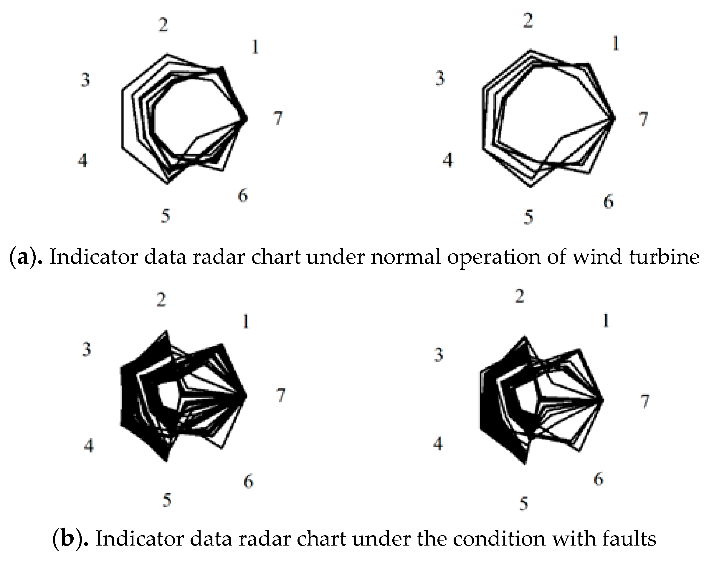
Based on the data extraction and processing as described above, two groups of radar charts are generated representing normal and faulty operation condition as shown in Figure 1. The wind speed is selected from 3 m/s to 20 m/s (cut-in and cut-off speed). Some of the data when wind speed is out of the range is removed. The collected data are plotted into the radar charts through the seven indicators selected and shown in Table 3, Table 5 and Table 7. In Figure 1, the numbers 1–7 represent the indicators, respectively, in Table 3, Table 5 and Table 7. The radar charts are distinguished by wind speed. For example, when the wind speed is 3 m/s, all indicators data under the condition is collected to plot the radar chart. In the graph, if the data is relatively stable, there are fewer curve lines to be observed as most of the frames are overlapping so that the pattern is regular and, otherwise, it is vice versa.
For each type of generator, converter and pitch system failure, 17,001 normal radar charts and 17,001 fault radar charts were generated. Since the selected fault indicators are all 7 and the operation process is consistent, we use the indicators data representing the generator’s normal and faulty operation conditions as an example to illustrate the analysis process. For the generator case, a total of 11,900 images of radar charts were selected for training the models and another 5101 images of radar charts were used for testing.
By making comparison analysis of the above radar charts, it is found that each indicator’s values are relatively stable and the distribution is regular under the normal generator operation whereas the indicator’s values are fluctuating and the chart distribution is relatively cluttered under faulty operation. The traditional analysis methods are mostly based on the training analysis of the data. In this paper, the convolutional neural network and support vector machine (SVM) methods are used to train models to identify the image characteristics during normal and fault operation. The fault detection accuracy is evaluated by analyzing the fault detection indices, which proves that the convolutional neural network is more suitable for detection of frequently occurred faults in wind turbine operation.

3. Development of Fault Detection Methods

3.1. Convolutional Neural Network Method for Fault Detection

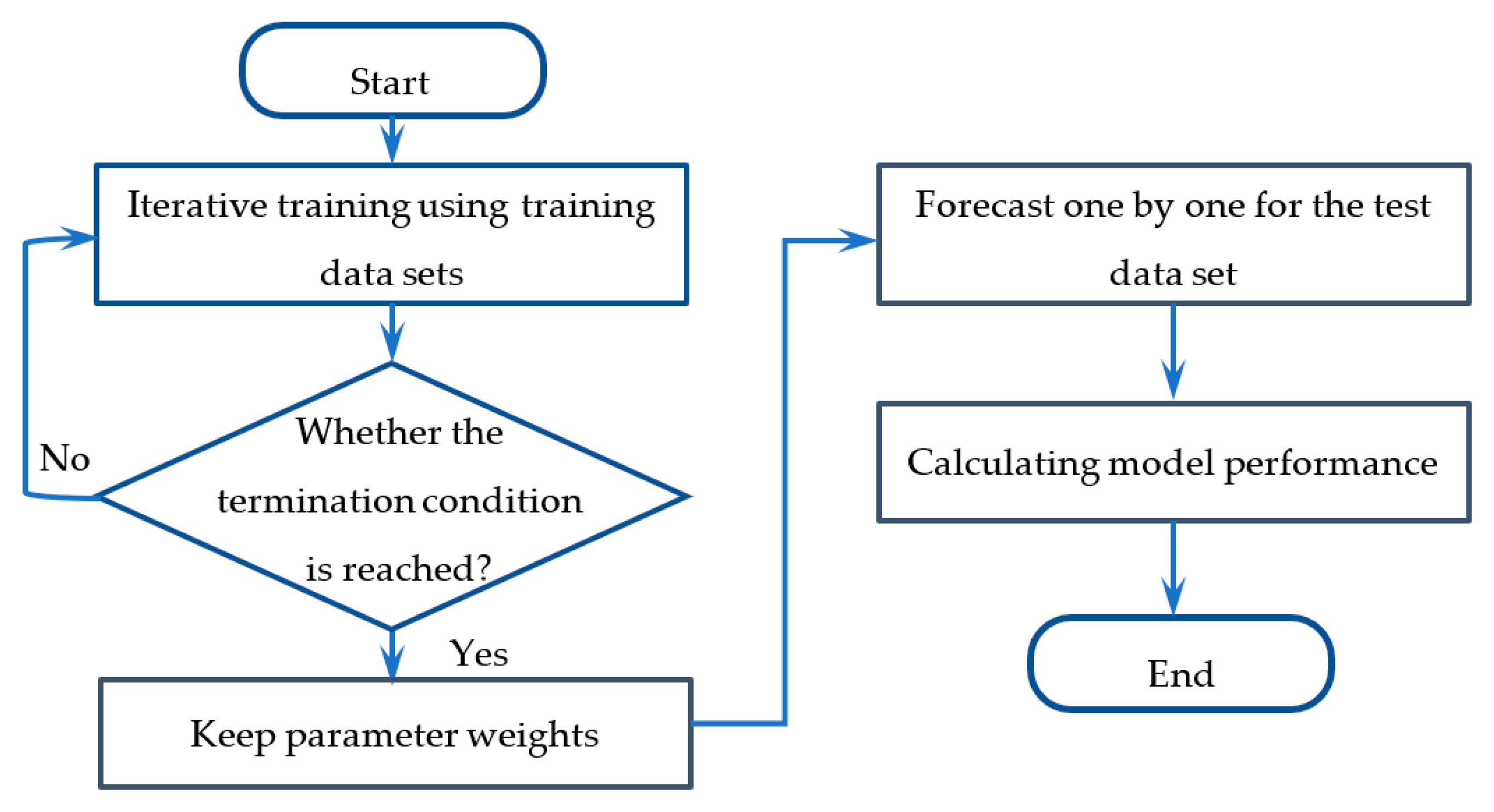
The core of the convolutional neural network is to train and learn from a large amount of sample data, and to extract the deep feature expression of the sample data through multiple iterations, and finally provide diagnosis according to different tasks and sample data [22]. This paper proposes a radar chart classification model based on the Restnet50 convolutional neural network structure to detect fault. The method includes preprocessing of the collected data, training of the target radar chart, and model performance testing. The training flow chart of the convolutional neural network model is shown in Figure 2.

3.1.1. Data Preprocessing and Data Set Construction for Training the Model

The procedure for data preprocessing and data set construction has been described in Section 2. In the training process of the convolutional neural network model, the characteristics of the images in the training data set are learned; as the number of network iterations increases, the network parameters are adjusted accordingly; thus, more representative image features are extracted, and finally the system model is determined for identification of fault condition.

3.1.2. Selection of Network Structure

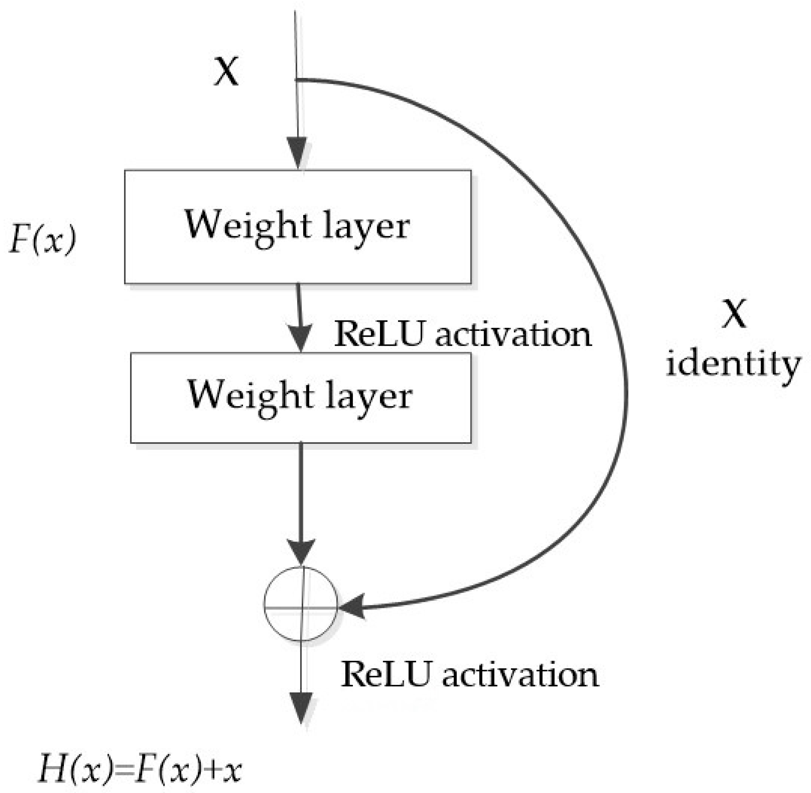
With increasing number of deep learning network layers, the features of different layers can be extracted. The more abstract the feature expression, the richer the semantic information. However, a simple increase in the number of original network layers in deep learning may result in gradient disappearance or gradient explosion. The traditional solutions generally use reasonable weight initialization and regularization methods to solve the gradient problem [23], but bring new problems of network performance degradation [24]. ResNet is a residual learning framework that can improve the network performance under the premise of increasing depth. ResNet’s residual unit structure diagram is shown in Figure 3 [25,26].
If the latter layer of the deep network is an identity map, the model can be degraded into a shallow network. However, using some layers directly to fit potential identity mapping functions such as: H(x) = x, will be more difficult. So, by designing the network as H ( x ) = F ( x ) + x , it turns the problem into learning a residual function F ( x ) = H ( x ) x . When F(x) = 0, it constitutes an identity map H ( x ) = x , for which it is easier to achieve residual fit.
Therefore, this paper adopts the residual network structure as shown in Figure 3 to improve the performance and accuracy of the network by increasing the network depth. The residual structure can be applied to solving the problem of gradient disappearance caused by the increase of network depth. Common residual network models include ResNet18, ResNet50, and ResNet101. As the number of layers increases, the amount of computation of the network increases accordingly. By considering the operation speed and accuracy, in this paper, the ResNet50 structure is selected as the backbone network [27].
a.
ResNet50 network structure
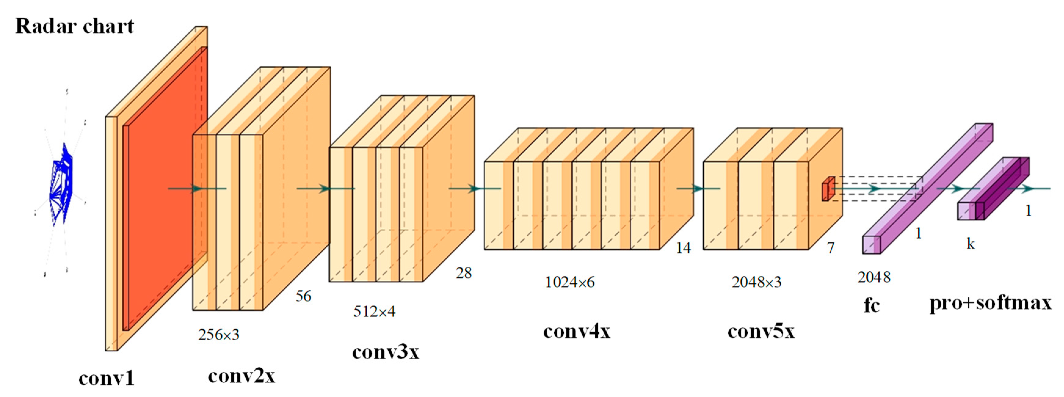
The overall structure of ResNet50 is shown in Table 11 [28] where conv1 is a 7 × 7 convolution kernel, a separate convolutional layer is formed, conv2x, conv3x, conv4, and conv5x are four residual groups, and each residual group contains three, four, six, and three residual units, respectively. The residual unit adopts a bottleneck layer design. In Table 11, FLOPs represents the amount of computation.
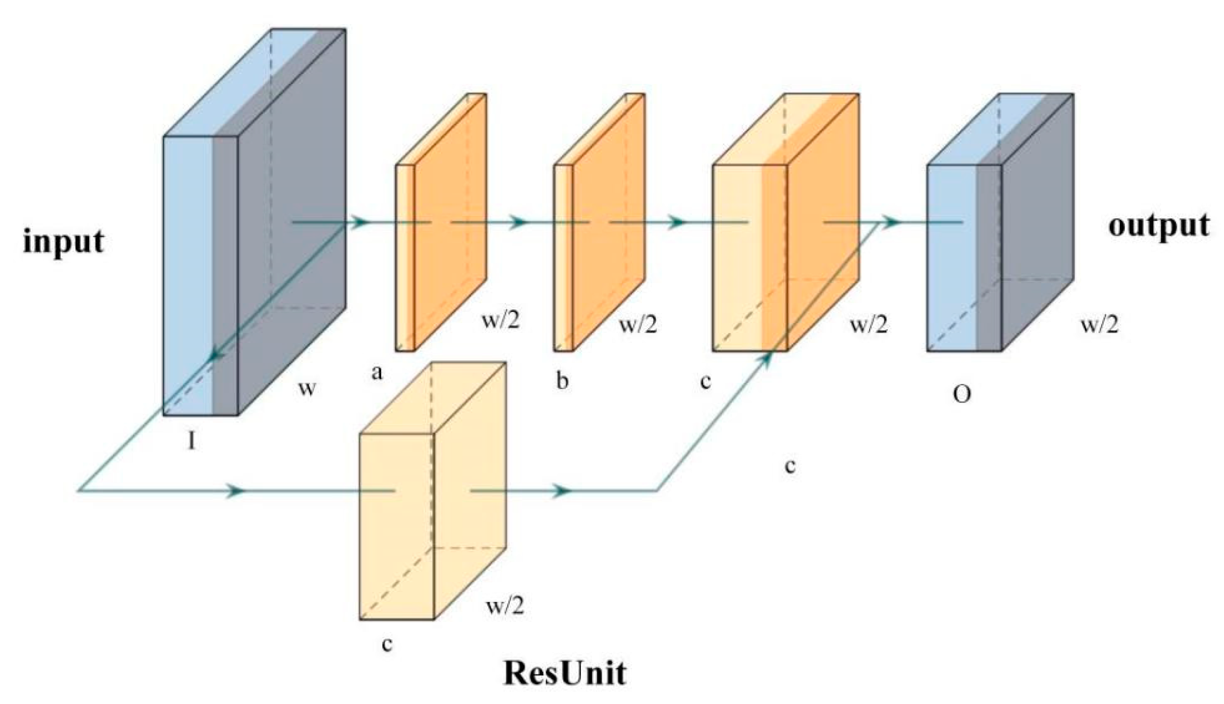
The residual component of the bottleneck layer design is shown in Figure 4. It consists of two convolution kernels, 1 × 1 and 3 × 3. The feature map input is first convolved to reduce the number of channels to 1/4 of the original, and then to be sent to the 3 × 3 convolutional layer. At the moment, the number of input channels is equal to the number of output channels, which is 1/4 of the original input channel number. Then through the 1 × 1 convolution kernel, it is finally increased by convolution to the original channel number, thereby reducing the computational complexity of the residual unit.
The network structure of ResNet50 is shown in Figure 5. The original input image size of ResNet50 is 224 × 224 × 3, and conv1 and max pooling are respectively down sampled, and the output feature size is 56 × 56 × 64. Then, after each residual group as described above, a down sampling is performed. The output of the last layer of the feature map is 7 × 7 × 2048, and then the 2048-dimensional feature vector is output through the global average pooling layer. Finally, the softMax layer is connected through the fully-connected layer for classification.
b.
Softmax classifier
The softmax classifier is an algorithm for classifying target variables. It takes the feature matrix of the fully connected layer as an input and outputs the probability value for each class. Suppose the input target variable is x i and the output target variable is marked as y i   ( i { 1 ,   2 ,   Λ ,   k } ) , k is the number of model output categories, and k ≥ 2. This paper classifies the frequently occurred failures, therefore, there are two operational states, i.e., normal and fault operating states, then here k = 2.
For input x i , using the hypothesis function to estimate the probability P ( y i = j | x i ) of the input corresponding to the two classifications as follows:
f θ ( x i ) = [ P ( y i = 1 | x i ; θ ) P ( y i = 2 | x i ; θ ) P ( y i = k | x i ; θ ) ] = 1 j = 1 k e θ j T x i [ e θ 1 T x i e θ 2 T x i e θ k T x i ]
Among them,   f θ ( x i ) is a hypothesis function, θ is the parameter of the softmax classifier. By normalizing 1 / ( j = 1 k e θ j T x i ) , the final probability sum is guaranteed to be 1.
c.
Cross entropy loss
The task is to determine a cross entropy as the loss function. The cross entropy characterizes the distance between the actual output (probability) and the expected output (probability), as shown in Equation (2):
H ( p , q ) = x ( p ( x ) log q ( x ) + ( 1 p ( x ) ) log ( 1 q ( x ) ) )
In the above formula, q is the desired output, p is the actual output, and H ( p ,   q ) is the cross entropy loss. When the actual output p is closer to the expected output q, the value of the loss function is smaller, and conversely, the value is larger.

3.1.3. The System Normal and Fault Image Feature Extraction

The convolutional layer extracts the features of the image by using convolution operation of the convolution kernel and the input image. The features extracted by different convolution kernels are different. The calculation formula of the convolution is:
Y p , q = i , j N k W i + k 1 2 , j + k 1 2 T X p + i , q + j
where, W R c × k × k denotes a k × k convolution kernel and X, Y R c × h × w denote the input and output variables, respectively; Y p , q R c denotes a point in output feature map; ( p , q ) denotes the location coordinate and N k = { ( i , j ) : i = { k 1 2 , , k 1 2 } , j = { k 1 2 , , k 1 2 } } defines a local neighborhood.
The pooling layer implements the down sampling operation on the input feature map. In this paper, the average pooling method averages the eigenvalues in the pooled kernel to play the role of feature aggregation, so that the model has translation invariance.
According to the radar image generated by SCADA data collected on site, the model is trained by ResNet50 network, and the model obtained by training is used to predict the operation of the future system state under fault operation.

3.2. SVM Detection Using Indicators Data Radar Chart

In this section, the SVM method is used to predict the above three types of system failures. The establishment of the data sets is the same as Section 2. SVM is a machine learning method which improves the generalization ability of machine learning through structural risk minimization [29].
For classification problems, assume the following training set: D = { ( x i ,   y i ) | i = 1 ,   2 ,   Λ ,   n } , among them, x i R n , y i { + 1 ,   1 } . It can be separated by hyperplane H: ω · x + b to maximize the hyperplane classification interval by solving the following quadratic optimization problems [30]:
min w , b 1 2 | | ω | | 2 = min w , b 1 2 ω T ω
s . t .   y i [ ω x i + b ] 1 0
Among them, i = 1, 2, ..., n; and ω and b are two parameters. For the even problem, it is a convex quadratic programming optimization problem, which can be obtained by solving the Lagrangian function, so the final decision function is:
f ( x )   =   sgn [ i = 1 n a i y i ( x i · x ) + b ] .
For the nonlinear case, the SVM first maps the input vector x to the high-dimensional feature space through the selected nonlinear mapping, and then constructs the hyperplane in this space for optimal linear classification.
The general process of using SVM to process image classification problem is as follows: (1) use appropriate algorithm to extract feature data from image data and establish data samples; (2) select training data set, test set and kernel function, and use the training data set to train classifier model; (3) use the test set to test the obtained model for fault detection; and (4) finally, the classification result and the classifier effect evaluation are obtained.
A flow diagram of the algorithm for processing image classification using SVM was given in [20], to which the readers are referred for a detailed discussion.

Construction of Confusion Matrix

A confusion matrix shows visualization effect of the performance of an algorithm through a specific matrix, which is a situation analysis table that summarizes the detection results of the classification model in machine learning. In the evaluation, the terms of TP, TN, FP, and FN are utilized. TP (True Positive) means that the true value is true and the predicted value is true; FN (False Negative) means that the true value is true and the predicted value is false; FP (False Positive) means that the true value is false and the predicted value is true; and TN (True Negative) means that the true value is false and the predicted value is false. The diagnosis performance of a SVM classifier is evaluated by the following five indices [20]:
a.
Accuracy
Accuracy = TP + TN TP + TN + FP + FN
b.
Diagnosed as true accuracy
Precision = TP TP + FP
c.
True to true accuracy
Recall = TP TP + FN
d.
True to false accuracy
Specificity = TN TN + FP
e.
Diagnosed as false accuracy
Negative   Detection =   TN TN + FN

3.3. Support Vector Regression (SVR) Detection Using the Indicator Data

In the previous study [20], the SVR method was applied to the fault detection of wind turbine pitch system. The same method is applied in this paper. The readers are referred to [20] for detailed discussions.

4. Detection Results and Analysis

The models developed using convolutional neural networks, SVM and SVR algorithms are applied to fault detection related to the three types of wind turbine failures. The ResNet50 structure is selected to develop the convolutional neural network model for fault detection. The input image size to the model is 224 × 224.

4.1. Convolutional Neural Network Detection Accuracy Analysis

Calculation of Detection Indices

The convolutional neural network method is used to detect faults in generator, converter and pitch system in operation. The results are shown below:
a.
Generator fault detection
The convolutional neural network ResNet50 is used to diagnose the operating states of the wind turbine generator. The values of the forecast indices, TP, FN, FP and TN are shown in Table 12 below.
Based on the data obtained above, the detection accuracy, the detection is true accuracy, the true is true accuracy, the true false accuracy, and the detection is false accuracy, are shown in Table 13.
b.
Converter fault detection
The convolutional neural network ResNet50 is used to identify the operating states of the wind turbine converter, and the indices, TP, FN, FP, and TN are given in Table 14 below.
The detection evaluation indices are shown in Table 15.
c.
Pitch system fault detection
Similar to the above, the detection indices and the detection performance indices are obtained as shown in Table 16 and Table 17, respectively.
By analyzing the data shown in Table 12, Table 13, Table 14, Table 15, Table 16 and Table 17, it is found that the method of using the convolutional neural network for model training can give a fault detection accuracy of over 94.8%.

4.2. SVM for Graphics Detection Accuracy Analysis

The SVM algorithm is used fault detection based on radar charts generated corresponding to different operating states of wind turbine generator, converter and pitch system by following the procedure described in Section 3.2.

4.2.1. Image Feature Extraction

a.
Image preprocessing
Before extracting the characteristics of the radar chart, the graphics of radar charts are first grayscaled and binarized, as shown in Figure 6. The grayscale values are set from 0 to 255. 0 means black while 255 means white. Then it is to classify the image pixels into black or white such that the pixels with grayscale values of less than 128 is classified as black and the others are deemed as white.
b.
Image feature extraction
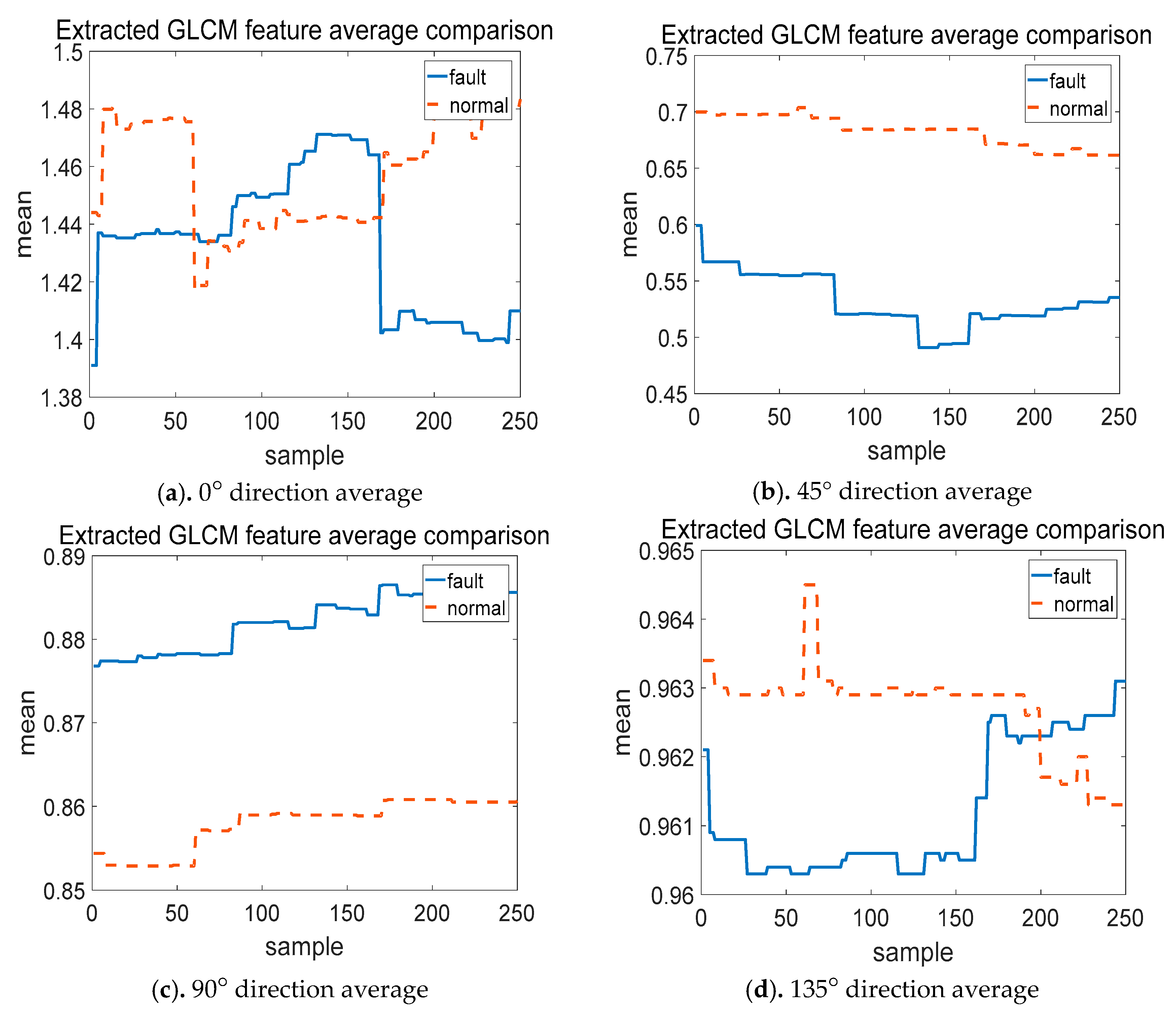
Here, the average value and the variance are used as the GLCM features of the extracted image. Due to too many image samples, it is difficult to observe the effect of GLCM mean and variance graphics. Therefore, 250 indicator data radar charts representing fault operation and 250 indicator data radar charts representing normal operation are taken as samples to compare the mean and variance of radar chart GLCM features. Figure 7 shows the GLCM feature average comparison. The feature extraction of the radar charts from four directions of θ = 0°, 45°, 90°, 135°; and the average value of each of the 250 samples of the indicator data radar charts under faulty and normal operation states, respectively, are calculated.
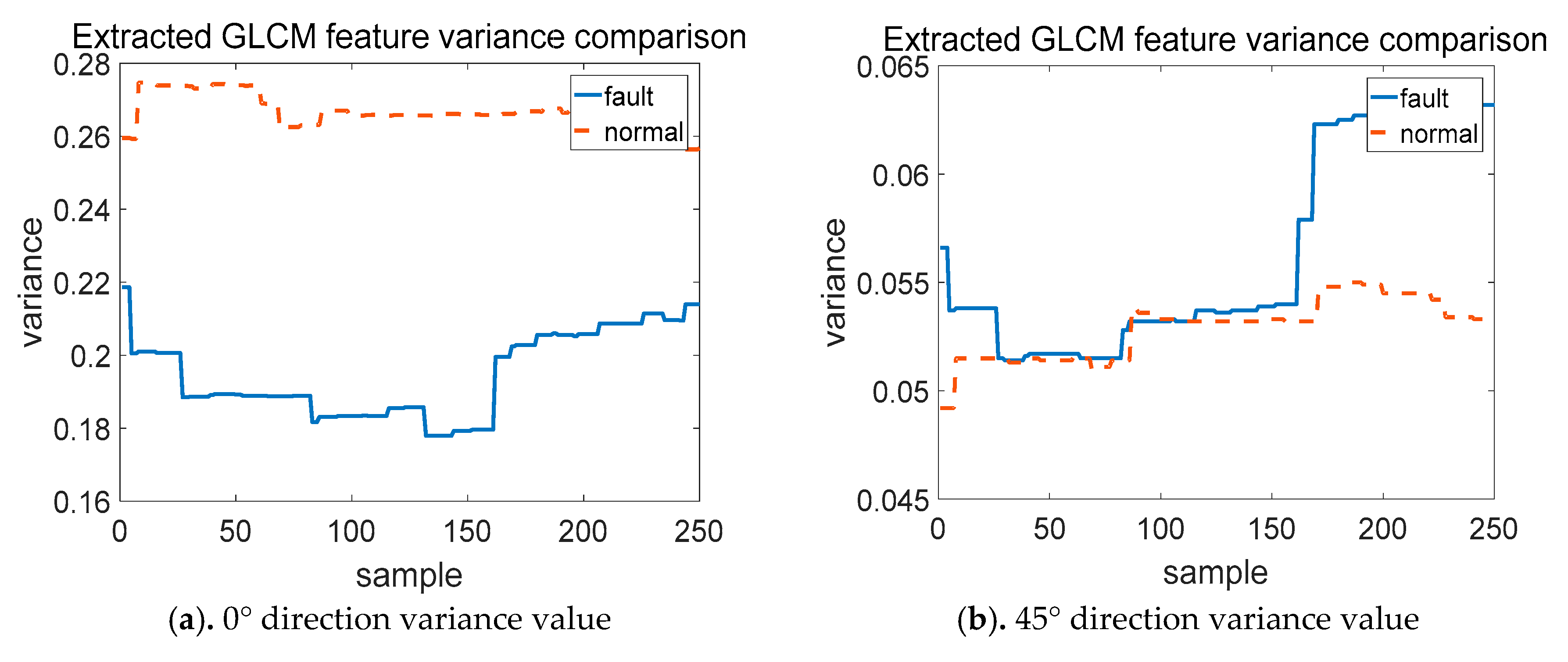
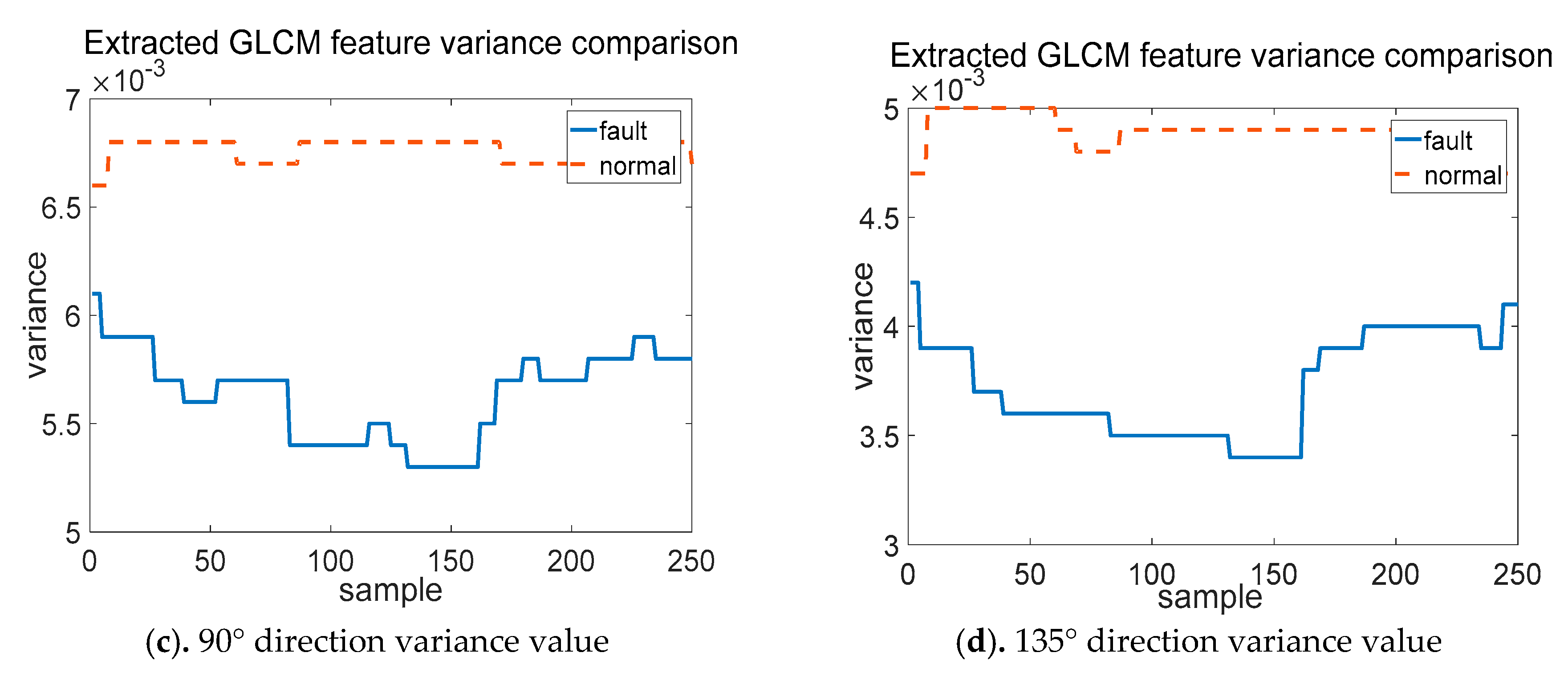
Figure 8 gives a comparison of GLCM feature variance values under two different wind turbine conditions. The feature extraction of the radar charts is from four directions of θ = 0°, 45°, 90°, 135°; and the variance values of 250 samples of the fault indicator data radar charts under fault and normal operation states, respectively, are calculated.
As shown in the Figure 7 and Figure 8 below, the mean and variance of the extracted features are significantly different under two different operation states of the system with and without faults. Since there is only some part of the overlap of the two curves shown in Figure 7a and Figure 8b, it proves that the SVM method is effective to detect the system operation status with and without faults.

4.2.2. Calculation of Detection Indices

The SVM method is used to detect the faults in generator, converter and pitch system. The results are shown in Table 18, Table 19, Table 20, Table 21, Table 22 and Table 23.
  • Generator fault detection
  • Converter fault detection
  • Pitch system fault detection
By analyzing the above indices, the detection accuracy of SVM method for fault detection is higher than 80%, which proves the feasibility of this method in application.

4.3. SVR Method for Fault Detection

When using the SVR method for fault detection based on the indicators data, the first step is to perform data preprocessing and remove the useless data. Then, use the preprocessed data to train the selected model.

4.3.1. Data Preprocessing

The indicators data is processed prior to model training. As described in Section 2, 200 sets of data are selected representing operation of generator, converter and pitch system with and without faults, respectively. The training data set includes 18,100 rows of the seven indicators data, and the test data set includes 9050 rows of the data.

4.3.2. Calculation of Detection Indices

The SVR method is used to detect faults in generator, converter and pitch system. The results are shown in Table 24, Table 25, Table 26, Table 27, Table 28 and Table 29.
a.
Generator fault detection
The forecast indices, TP, FN, FP, and TN for generator fault detection are shown in Table 24.
b.
Converter fault detection
c.
Pitch system fault detection
Using the SVR method, the fault detection accuracy for the generator and pitch system can reach more than 74% but the fault detection accuracy for the converter is only above 63%.

4.4. Comparison Analysis of the Three Fault Detection Methods

The detection evaluation index values by the convolutional neural network model, the SVM and the SVR method for detection of faults relating to the generator, converter and pitch system failure are summarized in Table 30, Table 31 and Table 32. In these tables, False alarm rate is given by (1 − Accuracy). It is a rate at which the wind turbine system health status is diagnosed wrongly.
a.
Comparison of detection evaluation indices for generator failure
The comparison of the detection evaluation indices for generator faults is given in Table 30 below.
It can be seen from the above table that the convolutional neural network and the SVM method are better than SVR model for detection of generator faults. The accuracy and the precision of the convolutional neural network are the highest among the three methods. The detection accuracy is 97.12 and the precision is 100. By comparing to the other two methods, the detection accuracy is obviously improved using the convolutional neural network method for detection of generator faults.
b.
Comparison of detection evaluation indices for converter failure
The detection evaluation index values for detection of the converter faults are shown in Table 31.
It can be seen from Table 31 that the detection accuracy (94.87%) and precision (100%) by the convolutional neural network are higher than the SVM method and the SVR model. The false alarm rate is also lower than the other methods. The Recall and Negative Detection values are also higher than the other two methods. Given the results shown in Table 31, it proves that the convolutional neural network is superior to the other two methods for detection of the converter system fault.
c.
Comparison of detection evaluation indices for pitch system faults
The detection evaluation index values for detection of the pitch system faults are shown in Table 32.
It can be seen from Table 32 that the detection accuracy for the pitch system faults by the convolutional neural network is higher than the SVM method and the SVR model. The false alarm rate is obviously reduced. Overall, it is better than the SVM method and the SVR model for detection of the pitch system faults.
It can be clearly seen from Table 30, Table 31 and Table 32 that the convolutional neural network can give the highest detection accuracy than the SVM method and the SVR model for detecting the generator, converter and pitch system faults. The convolutional neural network method is superior to the other two methods for detection of the faults related to the three subsystem failures.

5. Fault Detection Results and Analysis Using 10-min Data

Similar to Section 4, the developed three methods are applied to 10-min data. There are a total of 10 data sets corresponding to normal wind turbine operation and 10 data sets with faulty condition for each type of generator, pitch system and converter failure. Each data set is organized and presented in the same way as shown in Table 8, with 180 rows and seven columns and hence each data set sample size is 1260 (180 rows × 7 columns). The faulty data are the fault indicators data recorded 15 days ahead of a failure occurred. The fault detection results are shown in Table 33, Table 34 and Table 35 below.
Based on the results shown in Table 33, Table 34 and Table 35, we can verify that the convolutional neural network approach gives the highest accuracy than the SVM method and the SVR model for detecting the generator, converter and pitch system faults. The convolutional neural network method is superior to the other two methods in fault detection corresponding to the three subsystem failures.

6. Conclusions

This paper introduces the radar chart method into the wind turbine system fault detection methodology. The faults related to three frequently occurred system failures such as generator, converter and pitch system failures can be detected by the convolutional neural network, the SVM method and the SVR model developed in this paper. The convolutional neural network selects the ResNet50 structure as the backbone network. The procedure in detail for development of the convolutional neural network method is given. Through comparison of the detection evaluation indices for the fault detection by these three methods, it is clearly proved that the convolutional neural network method is superior to the SVM and the SVR method based on the preprocessing data.
For the faults related to the three types of wind turbine system failures, the detection accuracy by the convolutional neural network method is the highest, which is more than 94% using 10-s resolution data or 89% based on 10-min data; while it is close to 81% or 74% for the SVM method, and 63% or higher for the SVR model based on the preprocessing data. From the results obtained in this paper, it can be concluded that the fault detection method based on the convolutional neural network is more suitable for wind turbine system fault detection. In the future, the convolutional neural network and the SVM method will be applied to and tested for detection of other wind turbine faults based on the SCADA system data.
It is interesting to notice that the fault detection accuracy for pitch system is higher than generator and generator is better than converter by using each of the three methods. The pitch system faults are composed of both mechanical and electrical component faults while the generator failure is mainly caused by the electrical system faults and the converter system failure is mainly due to the failures of microelectronic components. A mechanical system fault typically presents a clearer degradation process (wear-out process).

Author Contributions

C.X. was responsible for theoretical development and developed algorithms; Z.L. contributed to the methodology and verified the modelling; X.Z. helped to collect data as required and develop algorithms together with C.X.; C.X. and T.Z. drafted the manuscript; T.Z. verified the algorithms and the results, finalized the paper and was responsible for paper revision and submission. Each author has contribution to the research approach development. All authors have read and agreed to the published version of the manuscript.

Funding

This work was partially supported by the National Natural Science Foundation of China (61703135; 61773151; 51577008); Hebei Natural Science Foundation (F2015202231); Youth Fund of Hebei Education Department (QN2019122); The Excellent Going Abroad Experts Training Program in Hebei Province.

Acknowledgments

The wind turbine operation data was collected from a wind farm in Hebei Province, China. The authors are grateful to the wind farm manager and engineers for kind support.

Conflicts of Interest

The authors declare no conflict of interest.

References

  1. Martin, B.A.; Bo, R.O.; Ole, W. Flexible non-linear predictive models for large-scale wind turbine diagnostics. Wind Energy 2017, 20, 753–764. [Google Scholar]
  2. Lu, B.; Li, Y.; Wu, X.; Yang, Z. A review of recent advances in wind turbine condition monitoring and fault diagnosis. In Proceedings of the 2009 IEEE Power Electronics and Machines in Wind Applications, Lincoln, NE, USA, 24–26 June 2009; pp. 1–7. [Google Scholar]
  3. Zhao, Y.Y.; Li, D.S.; Dong, A.; Kang, D.; Lv, Q.; Shang, L. Fault prediction and diagnosis of wind turbine generators using SCADA data. Energies 2017, 10, 1210. [Google Scholar] [CrossRef] [Green Version]
  4. Dao, P.B.; Staszewski, W.J.; Barszcz, T.; Uhl, T. Condition monitoring and fault detection in wind turbines based on cointegration analysis of SCADA data. Renew. Energy 2018, 116, 107–122. [Google Scholar] [CrossRef]
  5. Pérez, J.M.P.; Márquez, F.P.G.; Tobias, A.; Papaelias, M. Wind turbine reliability analysis. Renew. Sustain. Energy Rev. 2013, 23, 463–472. [Google Scholar] [CrossRef]
  6. Márquez, F.P.G.; Tobias, A.M.; Pérez, J.M.P.; Papaelias, M. Condition monitoring of wind turbines: Techniques and methods. Renew. Energy 2012, 46, 169–178. [Google Scholar] [CrossRef]
  7. Long, H.; Wang, L.; Zhang, Z.; Song, Z.; Xu, J. Data-driven wind turbine power generation performance monitoring. IEEE Trans. Ind. Electron. 2015, 62, 6627–6635. [Google Scholar] [CrossRef]
  8. Hwas, A.; Katebi, R. Model-based fault detection and isolation for wind turbine. In Proceedings of the 2012 UKACC International Conference on Control, Cardiff, UK, 3–5 September 2012; pp. 876–881. [Google Scholar]
  9. Ouyang, J.; Zhang, Z.; Tang, T.; Pang, M.; Li, M.; Zheng, D. Fault overload control method for high-proportion wind power transmission systems based on emergency acceleration of doubly-fed induction generator. IEEE Access 2019, 7, 32874–32883. [Google Scholar] [CrossRef]
  10. Li, J.; Li, M.; Zhang, J.; Jiang, G. Frequency-shift multiscale noise tuning stochastic resonance method for fault diagnosis of generator bearing in wind turbine. Measurement 2019, 133, 421–432. [Google Scholar] [CrossRef]
  11. Dong, H.; Yang, L.; Li, H. Small fault diagnosis of front-end speed controlled wind generator based on deep learning. WSEAS Trans. Circuits Syst. 2016, 15, 64–72. [Google Scholar]
  12. Hu, Y.; Shi, P.; Li, H.; Yang, C.; Liao, X. Health condition assessment of base-plate solder for multi-chip IGBT module in wind power converter. IEEE Access 2019, 7, 72134–72142. [Google Scholar] [CrossRef]
  13. Zhao, H.; Cheng, L. Open-circuit faults diagnosis in back-to-back converters of DF wind turbine. IET Renew. Power Gener. 2017, 11, 417–424. [Google Scholar] [CrossRef]
  14. Baygildina, E.; Smirnova, L.; Juntunen, R.; Murashko, K.; Mityakov, A.V.; Kuisma, M.; Pyrhönen, O.; Peltoniemi, P.; Hynynen, K.; Mityakov, V.Y.; et al. Condition monitoring of wind power converters using heat flux sensor. Int. Rev. Electr. Eng. 2016, 11, 239–246. [Google Scholar] [CrossRef]
  15. Wu, D.H.; Liu, W. A new fault diagnosis approach for the pitch system of wind turbines. Adv. Mech. Eng. 2017, 9, 1687814017703350. [Google Scholar] [CrossRef] [Green Version]
  16. Bi, R.; Zhou, C.K.; Hepburn, D.M. Detection and classification of faults in pitch-regulated wind turbine generators using normal behaviour models based on performance curves. Renew. Energy 2017, 105, 674–688. [Google Scholar] [CrossRef] [Green Version]
  17. Zhu, J.; Ma, K.; Hajizadeh, A.; Soltani, M.; Chen, Z. Fault detection and isolation for wind turbine electric pitch system. In Proceedings of the 2017 IEEE 12th International Conference on Power Electronics and Drive Systems (PEDS), Honolulu, HI, USA, 12–15 December 2017; pp. 618–623. [Google Scholar]
  18. Wu, D.; Liu, W.; Zhai, Y.; Shen, Y. Fault diagnosis for the pitch system of wind turbines using the observer-based multi-innovation stochastic gradient algorithm. In Theory, Methodology, Tools and Applications for Modeling and Simulation of Complex Systems; Springer: Singapore, 2016; pp. 526–538. [Google Scholar]
  19. Chen, B.; Matthews, P.C.; Tavner, P.J. Wind turbine pitch faults prognosis using a-priori knowledge-based ANFIS. Expert Syst. Appl. 2013, 40, 6863–6876. [Google Scholar] [CrossRef]
  20. Xiao, C.; Liu, Z.J.; Zhang, T.L.; Zhang, L. On fault prediction for wind turbine pitch system using radar chart and support vector machine approach. Energies 2019, 12, 2693. [Google Scholar] [CrossRef] [Green Version]
  21. Yang, Z. Research on Fault Early Warning Method Using Data Analysis for Wind Turbine Pitch System. Master’s Thesis, North China Electric Power University, Beijing, China, 2015. [Google Scholar]
  22. Simonyan, K.; Zisserman, A. Very deep convolutional networks for large-scale image recognition. arXiv 2014, arXiv:1409.1556. [Google Scholar]
  23. Ioffe, S.; Szegedy, C. Batch normalization: Accelerating deep network training by reducing internal covariate shift. In Proceedings of the 32nd International Conference on Machine Learning, Lille, France, 6–11 July 2015. [Google Scholar]
  24. He, K.; Zhang, X.; Ren, S.; Sun, J. Deep residual learning for image recognition. In Proceedings of the IEEE Conference on Computer Vision and Pattern Recognition, Las Vegas, NV, USA, 27–30 June 2016; pp. 770–778. [Google Scholar]
  25. Zagoruyko, S.; Komodakis, N. Wide residual networks. In Proceedings of the BMVC 2016, York, UK, 19–22 September 2016; pp. 87.1–87.12. [Google Scholar]
  26. He, K.; Zhang, X.; Ren, S.; Sun, J. Identity mappings in deep residual networks. In European Conference on Computer Vision; Springer: Cham, Switzerland, 2016; pp. 630–645. [Google Scholar]
  27. Guo, Y.; Su, P.F.; Wu, Y.F.; Guo, J. Object detection and location of robot based on Faster R-CNN. Huazhong Univ. Sci. Technol. 2018, 46, 55–59. [Google Scholar]
  28. Wang, H.; Li, X.; Liu, X.F.; Xu, W.L. Classification of breast cancer histopathological images based on ResNet50 Network. J. China Univ. Metrol. 2019, 30, 72–77. [Google Scholar]
  29. Liao, M.; Zhao, Y.Q.; Zeng, Y.Z.; Huang, Z.C.; Zhang, B.K.; Zou, B.J. Automatic segmentation for cell images bases on support vector machine and ellipse fitting. J. Zhejiang Univ. 2017, 51, 722–728. [Google Scholar]
  30. Shen, Y.X.; Zhou, W.J.; Ji, Z.C.; Wu, D.H. Fault diagnosis of converter used in wind power generation based on wavelet packet analysis and SVM. Acta Energ. Sol. Sin. 2015, 36, 785–791. [Google Scholar]
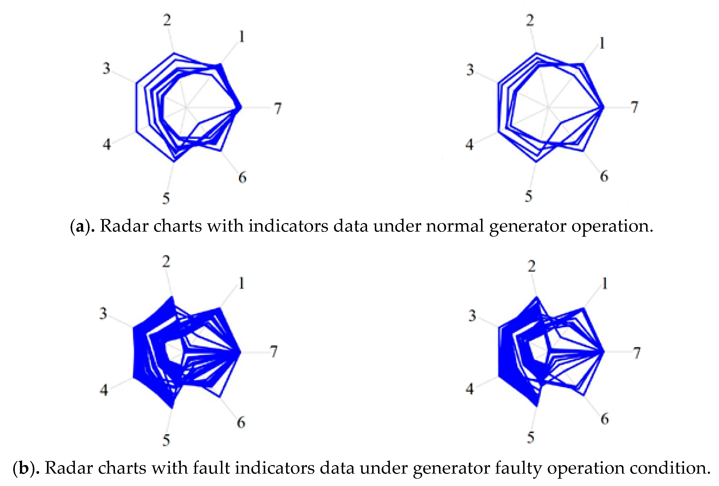
Figure 1. Indicators data radar chart.
Energies 13 00460 g001
Figure 2. Training flow diagram of the convolutional neural network model.
Energies 13 00460 g002
Figure 3. Residual unit structure diagram.
Energies 13 00460 g003
Figure 4. Bottleneck residual unit.
Energies 13 00460 g004
Figure 5. ResNet50 network structure.
Energies 13 00460 g005
Figure 6. Indicator data radar chart preprocessing.
Energies 13 00460 g006
Figure 7. GLCM feature average comparison chart.
Energies 13 00460 g007
Figure 8. GLCM feature variance value comparison chart.
Energies 13 00460 g008aEnergies 13 00460 g008b
Table 1. Percentage of downtime per wind turbine subsystem [3].
GeneratorConverterBlades/Pitch SystemScheduled StopYaw SystemGearboxOthers
37%19%12%10%4%3%15%
Table 2. Main faults of generator.
Serial No.Generator Fault Type
1Generator air cooling fan fails
2Generator bearing temperature is out of limits
3Generator encoder fault
4Generator encoder shielded line
5Generator winding temperature overrun
Table 3. Generator fault related parameter indicators.
Serial No.1234567
IndexWind speedRotor speedGenerator winding temperatureGenerator bearing temperatureGenerator cooling air temperatureGrid powerGrid reactive power
Table 4. Main faults of converter.
Serial No.Main Faults of Converter
1The grid side converter voltage is faulty, and the inverter module wiring is loose
2Rotor side converter fault
3Grid-side converter voltage failure, inverter Hall sensor damage
4The grid side converter is ready to be closed, and the CB504 wiring is loose
5The grid side converter is ready to be closed and the wiring is faulty
Table 5. Indicator parameters related to converter failure.
Serial No.1234567
IndexWind speedRotor speedGrid powerGenerator rotor speedConverter powerConverter Ctrl torque set pointGenerator torque
Table 6. Main faults of the pitch system.
Serial No.Pitch System Fault Type
1Pitch 90° position sensor fault
2Pitch safety chain fault
33° position sensor fault of pitch paddle 1
4Pitch emergency stop fault
5Pitch motor high temperature fault
Table 7. Indicator parameters related to pitch system failure.
Serial No.1234567
IndexWind speedWind directionRotor speedRotor positionOutput powerGrid frequencyPitch angle
Table 8. SCADA system indicator variable data when the system is in generator faulty operation.
Serial NumberWind Speed (m/s)Rotor Speed (rad/min)Generator Winding Temperature (°C)Generator Bearing Temperature (°C)Generator Cooling Air Temperature (°C)Grid Power (kW)Grid
Reactive Power
(kW)
15.0110.47150.937.131.1124.8184.7
25.5510.4450.837.131.1138184.1
34.8910.4550.837.131.1141.6188.8
45.8810.5150.837.131.1147179.5
54.9310.4250.837.131.1147182.7
65.6510.4750.73731.1149.4179.3
1781.660.014128.93600
1791.510.014128.93600
1802.030.0141293600
1811.9604128.93600
Table 9. SCADA system indicator variable data when the system is in converter faulty operation.
Serial NumberWind Speed (m/s)Rotor Speed (rad/min)Grid
Power
(kW)
Generator Rotor Speed
(rad/min)
Converter Input
Power
(kW)
Converter Ctrl Torque Set Point
(N·m)
Generator Torque
(N·m)
17.6114.33428.41440.5430.834.5533.81
25.6814.42441.61448.9450.234.9135.13
34.9114.184141420419.133.4233.41
45.0813.81387.61387.639432.0732.03
54.3112.983241304.3329.628.2828.55
64.8512.54292.21260.5297.326.3526.61
1783.2210.3897.81043.399.610.6710.6
1793.0810.4181.11045.985.38.998.97
1803.0610.47691051.871.47.727.78
1813.3810.47931052.394.310.5410.29
Table 10. SCADA system indicator variable data when the system is in pitch faulty operation.
Serial NumberWind Speed (m/s)Wind Direction (°)Rotor Speed (rad/min)Rotor Position (°)Output Power
(kW)
Grid Frequency
(Hz)
Pitch Angle
(°)
15.77196.110.4193.4168.6505.02
25.96177.110.574.9174.6505.02
35.96177.110.574.9174.6505.02
45.46173.310.4235.8152.4505.02
55.46173.310.4235.8152.4505.02
65.36162.410.479.5135.6505.02
1781.29188.10.1352.1049.988.9
1790.64152.10.1354.3050.188.9
1800.79126.70.1357.1050.188.9
1810.71137.80.1358.3050.188.9
Table 11. ResNet50 network structure.
Layer NameOutput Size50-Layer
conv1 112 × 112 7 × 7, 64, stride 2
3 × 3 max pool, stride 2
conv2x 56 × 56 [ 1 × 1 ,     64 3 × 3 ,     64     1 × 1 ,     256 ] × 3
conv3x 28 × 28 [ 1 × 1 ,     128 3 × 3 ,     128 1 × 1 ,     512 ] × 4
conv4x 14 × 14 [ 1 × 1 ,     256 3 × 3 ,     256     1 × 1 ,     1024 ] × 6
conv5x 7 × 7 [ 1 × 1 ,     512 3 × 3 ,     512     1 × 1 ,     2048 ] × 3
1 × 1 average pool, 1000-d fc, softmax
Floating points operations (FLOPs) 3.8 × 10 9
Table 12. Forecast indices value.
IndexTPFNFPTN
Numerical value480729405101
Table 13. Detection evaluation indices.
IndexAccuracyPrecisionRecallSpecificityNegative Detection
Value (%)97.1210094.2410094.55
Table 14. Forecast indices value.
IndexTPFNFPTN
Numerical value457852305101
Table 15. Detection evaluation indices.
IndexAccuracyPrecisionRecallSpecificityNegative Detection
Value (%)94.8710089.7510090.7
Table 16. Forecast indices value.
IndexTPFNFPTN
Numerical value51010905011
Table 17. Detection evaluation indices.
IndexAccuracyPrecisionRecallSpecificityNegative Detection
Value (%)99.1198.2710098.24100
Table 18. Forecast indices value.
IndexTPFNFPTN
Numerical value5057446584443
Table 19. Detection evaluation indices.
IndexAccuracyPrecisionRecallSpecificityNegative Detection
Value (%)93.1288.4999.1487.199.02
Table 20. Forecast indices value.
IndexTPFNFPTN
Numerical value337917222264875
Table 21. Detection evaluation indices.
IndexAccuracyPrecisionRecallSpecificityNegative Detection
Value (%)80.9193.7366.2495.5773.89
Table 22. Forecast indices value.
IndexTPFNFPTN
Numerical value48742541114990
Table 23. Detection evaluation indices.
IndexAccuracyPrecisionRecallSpecificityNegative Detection
Value (%)96.4297.7595.5597.8295.16
Table 24. Forecast indices value.
IndexTPFNFPTN
Numerical value82068449558095
Table 25. Detection evaluation indices.
IndexAccuracyPrecisionRecallSpecificityNegative Detection
Numerical value (%)89.9489.5890.6789.4590.56
Table 26. Forecast indices value.
IndexTPFNFPTN
Numerical value3610544012007850
Table 27. Detection evaluation indices.
IndexAccuracyPrecisionRecallSpecificityNegative Detection
Value (%)63.3175.0539.8986.7459.07
Table 28. Forecast indices value.
IndexTPFNFPTN
Numerical value5651339911967854
Table 29. Detection evaluation indices.
IndexAccuracyPrecisionRecallSpecificityNegative Detection
Value (%) 74.6182.5362.4486.7869.79
Table 30. Comparison of detection evaluation indices among the three methods for generator faults.
ApproachAccuracyPrecisionRecallSpecificityNegative
Detection
False Alarm
Rate
Convolutional neural network (%)97.1210094.2410094.552.88
SVM method (%)93.1288.4999.1487.199.026.88
SVR model (%)89.9489.5890.6789.4590.5610.06
Table 31. Comparison of detection evaluation indices among the three methods for converter faults.
ApproachAccuracyPrecisionRecallSpecificityNegative
Detection
False Alarm
Rate
Convolutional neural network (%)94.8710089.7510090.75.13
SVM method (%)80.9193.7366.2495.5773.8919.09
SVR model (%)63.3175.0539.8986.7459.0736.69
Table 32. Comparison of detection evaluation indices among the three methods for pitch system faults.
ApproachAccuracyPrecisionRecallSpecificityNegative
Detection
False Alarm
Rate
Convolutional neural network (%)99.1198.2710098.241000.89
SVM method (%) 96.4297.7595.5597.8295.163.58
SVR model (%)74.6182.5362.4486.7869.7925.39
Table 33. Comparison of detection evaluation indices among the three methods for generator faults.
ApproachAccuracyPrecisionRecallSpecificityNegative
Detection
False Alarm
Rate
Convolutional neural network (%) 97.8798.2297.5298.2397.542.13
SVM method (%)79.0385.9669.3888.6774.3320.97
SVR model (%)73.8978.1466.3381.4470.7526.11
Table 34. Comparison of detection evaluation indices among the three methods for converter faults.
ApproachAccuracyPrecisionRecallSpecificityNegative
Detection
False Alarm
Rate
Convolutional neural network (%)89.0399.178.7699.2982.3810.97
SVM method (%)74.0770.1883.7264.4279.8225.93
SVR model (%)64.7874.7244.6784.8960.5435.22
Table 35. Comparison of detection evaluation indices among the three methods for pitch system faults.
ApproachAccuracyPrecisionRecallSpecificityNegative
Detection
False alarm
rate
Convolutional neural network (%)98.41 96.9210096.821001.59
SVM method (%) 89.4982.6310078.9810010.51
SVR model (%)80.9478.390.2271.6787.9919.06