Homogeneous Flux Distribution in High-Flux Solar Furnaces


Abstract

1. Introduction
2. Experimental and Modelling Details
3. Solar Furnace Flux Distribution
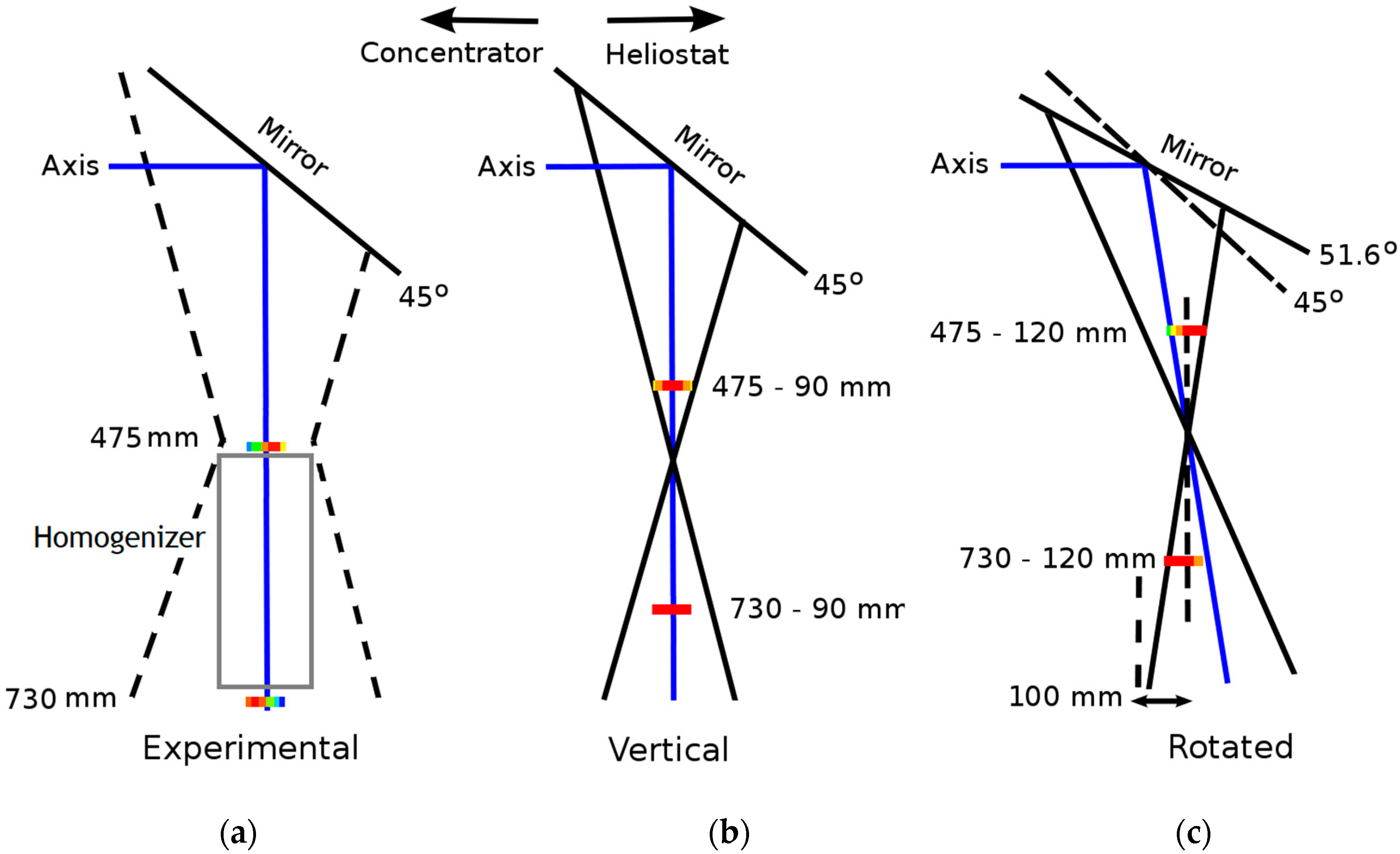
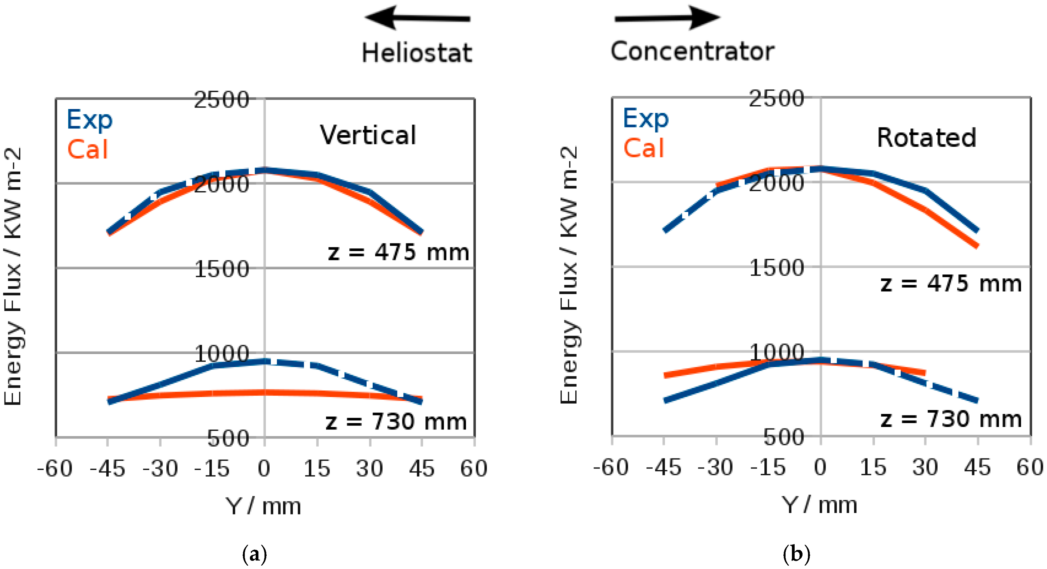
3.1. Vertical Beam Modelling
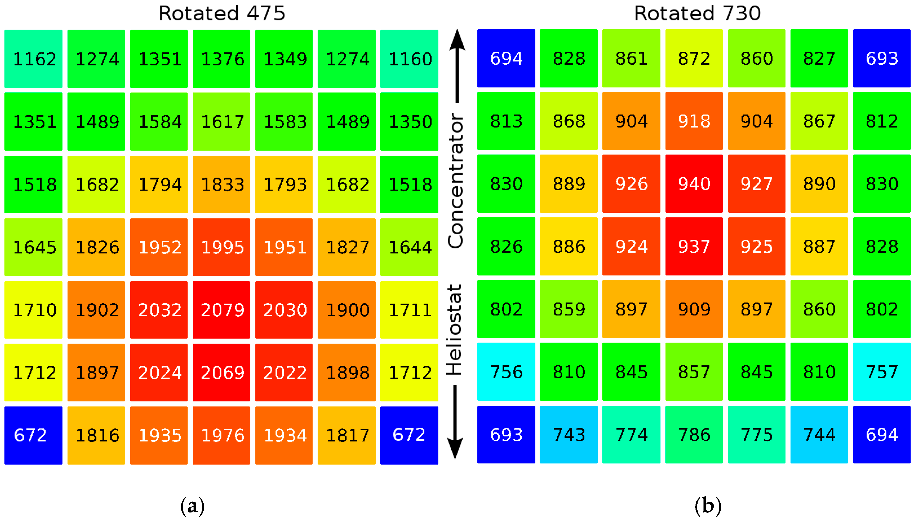
3.2. Rotated Beam Modelling
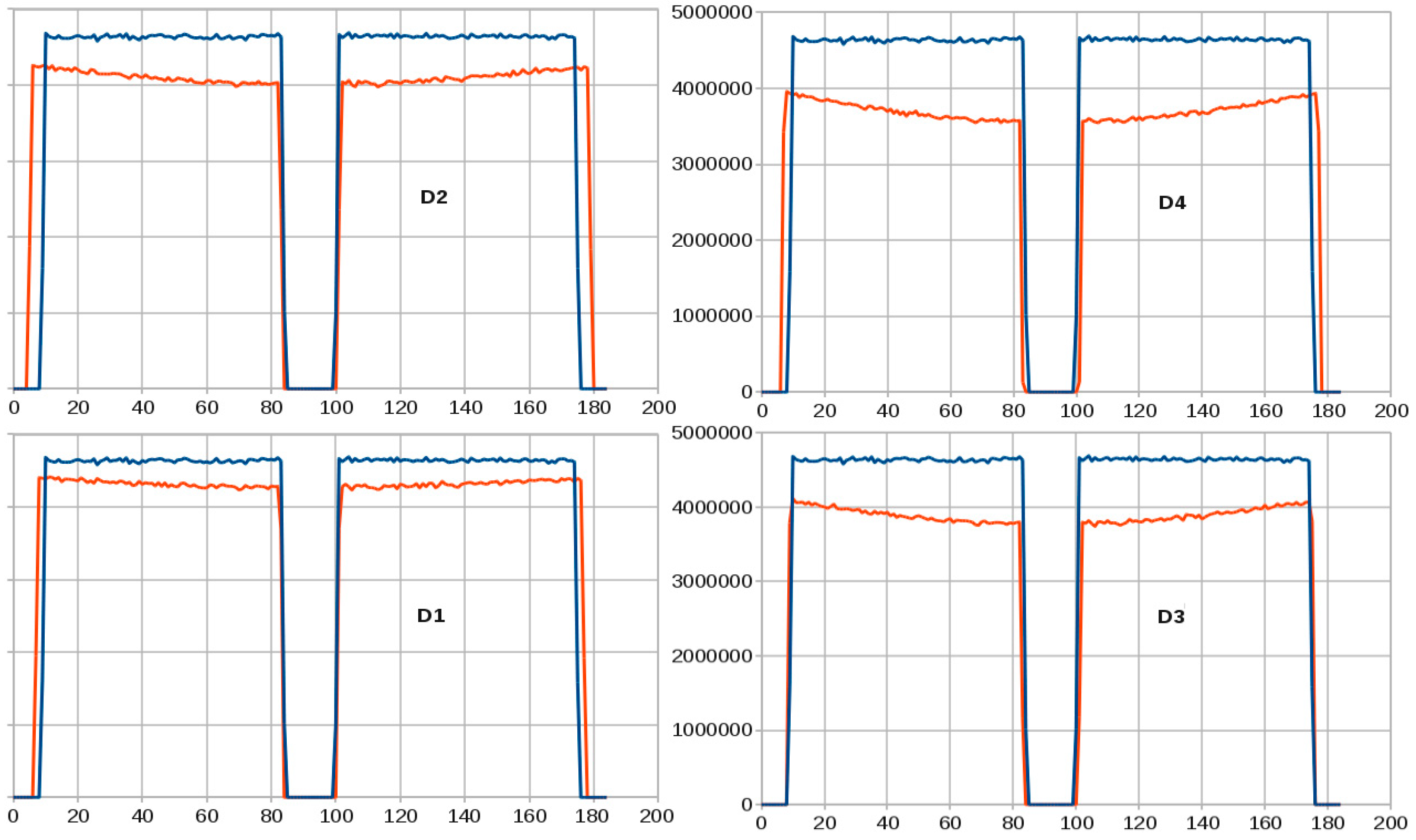
4. Homogeniser Flux Distribution
5. Double Paraboloid Flux Distribution
5.1. Parallel Rays
5.2. Non-Parallel Rays
5.3. Calibrated Rays
5.4. Final Remarks
6. Conclusions
Author Contributions
Funding
Conflicts of Interest
References
- Răboacă, M.S.; Badea, G.; Enache, A.; Filote, C.; Răsoi, G.; Rata, M.; Lavric, A.; Felseghi, R. Concentrating solar power technologies. Energies 2019, 12, 1048. [Google Scholar] [CrossRef]
- Abanades, S. Metal oxides applied to thermochemical water-splitting for hydrogen production using concentrated solar energy. ChemEngineering 2019, 3, 63. [Google Scholar] [CrossRef]
- Levêque, G.; Bader, R.; Lipinski, W.; Haussener, S. High-flux optical systems for solar thermochemistry. Sol. Energy 2017, 156, 133–148. [Google Scholar] [CrossRef]
- Yadav, D.; Banerjee, R. A review of solar thermochemical processes. Renew. Sustain. Energy Rev. 2016, 54, 497–532. [Google Scholar] [CrossRef]
- Rosa, L.G. Solar heat for materials processing: A review on recent achievements and a prospect on future trends. ChemEngineering 2019, 3, 83. [Google Scholar] [CrossRef]
- Fernández-González, D.; Ruiz-Bustinza, I.; González-Gasca, C.; Piñuela-Noval, J.; Mochón-Csataños, J.; Sancho-Gorostiaga, J.; Verdeja, L.F. Concentrated solar energy applications in materials science and metallurgy. Sol. Energy 2018, 170, 520–540. [Google Scholar] [CrossRef]
- Douale, P.; Serror, S.; Duval, R.M.P.; Serra, J.J.; Felder, E. Thermal shocks on an electrolytic chromium coating in a solar furnace. J. Phys. IV 1999, 9, 429–434. [Google Scholar] [CrossRef]
- Kováčik, J.; Emmer, S.; Rodriguez, J.; Cañadas, I. Solar furnace: Thermal shock behaviour of TiB2 coating on steel. In Proceedings of the METAL 2014, Brno, Czech Republic, 21–23 May 2014; pp. 863–868. Available online: https://www.academia.edu/24388464/Solar_Furnace_Thermal_Shock_Behaviour_of_TIB2_Coating_on_Steel (accessed on 12 December 2019).
- Sallaberry, F.; García de Jalón, A.; Zaversky, F.; Vázquez, A.J.; López-Delgado, A.; Tamayo, A.; Mazo, M.A. Towards standard testing materials for high temperature solar receivers. Energy Procedia 2015, 69, 532–542. [Google Scholar] [CrossRef][Green Version]
- Rosa, L.G.; Rodríguez, J.; Pereira, J.; Fernandes, J.C. Thermal cycling behaviour of dense monolithic alumina. In Proceedings of the Second International Conference on Materials Chemistry and Environmental Protection—MEEP 2018, Sanya, China, 23–25 November 2018; pp. 173–179, ISBN 978-989-758-360-5. [Google Scholar] [CrossRef]
- Oliveira, F.A.C.; Fernandes, J.C.; Galindo, J.; Rodríguez, J.; Canãdas, I.; Rosa, L.G. Thermal resistance of solar volumetric absorbers made of mullite, brown alumina and ceria foams under concentrated solar radiation. Sol. Energy Mater. Sol. Cells 2019, 194, 121–129. [Google Scholar] [CrossRef]
- Balat-Pichelin, M.; Eck, J.; Sans, J.L. Thermal radiative properties of carbon materials under high temperature and vacuum ultra-violet (VUV) radiation for the heat shield of the Solar Probe Plus mission. Appl. Surf. Sci. 2012, 258, 2829–2835. [Google Scholar] [CrossRef]
- Sani, E.; Mercatelli, L.; Jafrancesco, D.; Sans, J.L.; Sciti, D. Ultra-high temperature ceramics for solar receivers: Spectral and high-temperature emittance characterization. J. Eur. Opt. Soc. Rap. Publ. 2012, 7, 12052. [Google Scholar] [CrossRef]
- Pereira, J.C.G.; Fernandes, J.C.; Rosa, L.G. Mathematical Models for Simulation and Optimization of High-Flux Solar Furnaces. Math. Comput. Appl. 2019, 24, 65. [Google Scholar] [CrossRef]
- Monreal, A.; Riveros-Rosas, D.; Sanchez, M. Analysis of the influence of the site in the final energy cost of solar furnaces for its use in industrial applications. Sol. Energy 2015, 118, 286–294. [Google Scholar] [CrossRef]
- Bushra, N.; Hartmann, T. A review of state-of-the-art reflective two-stage solar concentrators: Technology categorization and research trends. Renew. Sustain. Energy Rev. 2019, 114, 109307. [Google Scholar] [CrossRef]
- Nakamura, T. Optical waveguide system for solar power applications in space. In Nonimaging Optics: Efficient Design for Illumination and Solar Concentration VI; International Society for Optics and Photonics: San Francisco, CA, USA, 2009; Volume 7423, p. 74230C. [Google Scholar] [CrossRef]
- Nakamura, T.; Smith, B.K. Solar thermal system for lunar ISRU applications: Development and field operation at Mauna Kea, HI. In Proceedings of the SPIE 8124, Nonimaging Optics: Efficient Design for Illumination and Solar Concentration VIII, San Diego, CA, USA, 21–25 August 2011; Volume 81240B. [Google Scholar] [CrossRef]
- Nakamura, T.; Smith, B.K.; Irvin, B.R. Optical waveguide solar power system for material processing in space. J. Aerosp. Eng. 2015, 28, 04014051. [Google Scholar] [CrossRef]
- Rodriguez, J.; Cañadas, I.; Monterreal, R.; Enrique, R.; Galindo, J. PSA SF60 solar furnace renewed. AIP Conf. Proc. 2019, 2126, 030046. [Google Scholar] [CrossRef]
- Ballestrín, J.; Ulmer, S.; Morales, A.; Barnes, A.; Langley, L.W.; Rodríguez, M. Systematic error in the measurement of very high solar irradiance. Sol. Energy Mater. Sol. Cells 2003, 80, 375–381. [Google Scholar] [CrossRef]
- Solar Limb Darkening. Available online: http://exoplanet-diagrams.blogspot.com/2015/07/solar-limb-darkening.html (accessed on 13 December 2019).
- Buie, D.; Monger, A.G.; Dey, C.J. Sunshape distributions for terrestrial solar simulations. Sol. Energy 2003, 74, 113–122. [Google Scholar] [CrossRef]
- Luque, S.; Santiago, S.; Gomez-Garcia, F.; Romero, M.; Gonzalez-Aguilar, J. A new calorimetric facility to investigate radiative-convective heat exchangers for concentrated solar power applications. Int. J. Energy Res. 2018, 42, 966–976. [Google Scholar] [CrossRef]
- Luque, S.; Bai, F.; González-Aguilar, J.; Wang, Z.; Romero, M. A parametric experimental study of aerothermal performance and efficiency in monolithic volumetric absorbers. AIP Conf. Proc. 2017, 1850, 030034. [Google Scholar] [CrossRef]
- Gomez-Garcia, F.; Santiago, S.; Luque, S.; Romero, M.; Gonzalez-Aguilar, J. A new laboratory-scale experimental facility for detailed aerothermal characterizations of volumetric absorbers. AIP Conf. Proc. 2016, 1734, 030018. [Google Scholar] [CrossRef]


| Measurement Conditions | Power (kW) | Flux Average (kW/m2) | Flux Standard Deviation (kW/m2) | Coefficient of Variation (CV) |
|---|---|---|---|---|
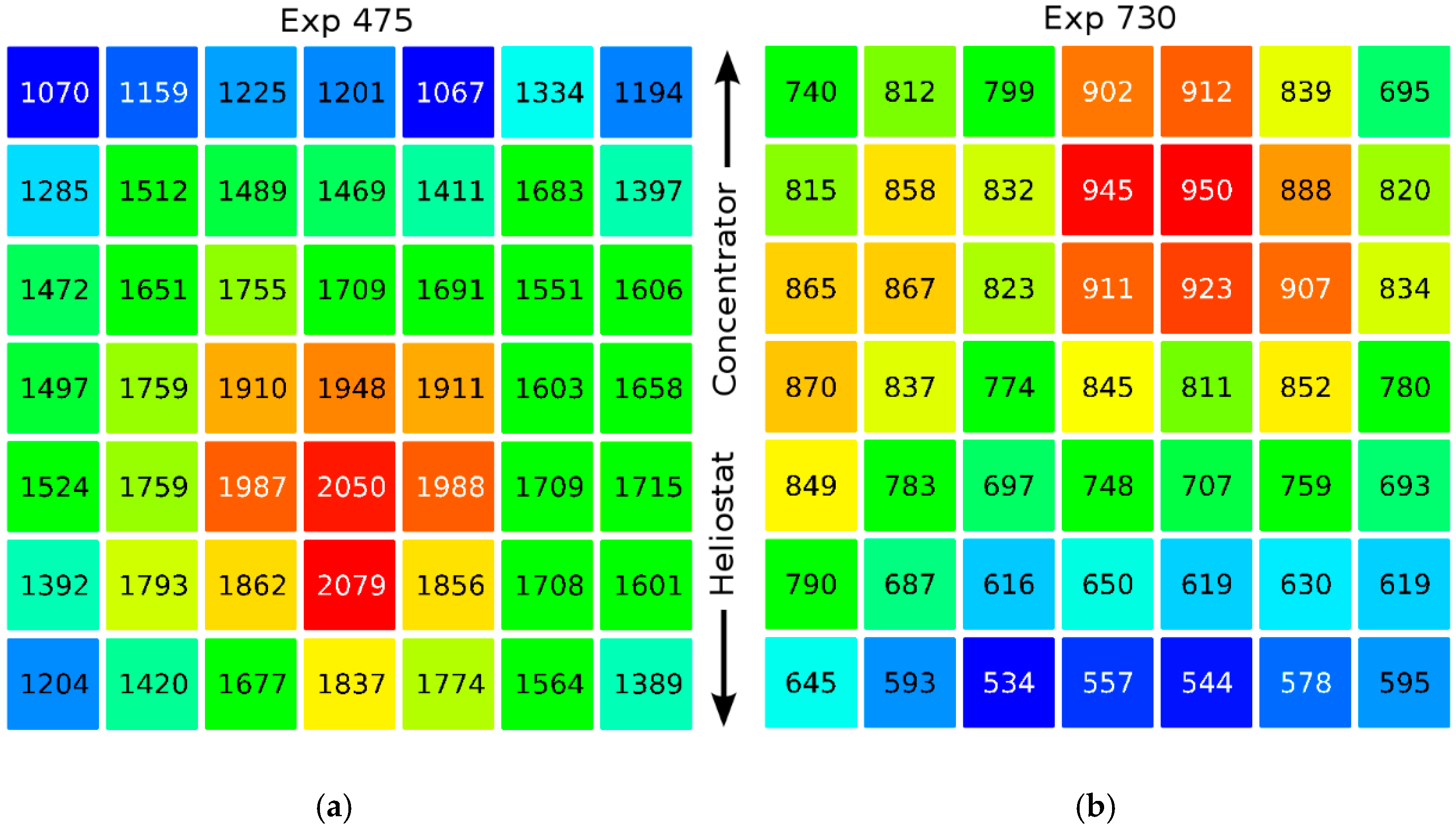
| z = 475 mm | 17.6 | 1594.0 | 261.2 | 0.16 |
| z = 730 mm | 8.5 | 767.3 | 117.2 | 0.15 |
| Homogeniser z = 730 | 24.7 | 2236.8 | 198.1 | 0.09 |
© 2020 by the authors. Licensee MDPI, Basel, Switzerland. This article is an open access article distributed under the terms and conditions of the Creative Commons Attribution (CC BY) license (http://creativecommons.org/licenses/by/4.0/).
Share and Cite
Pereira, J.C.G.; Rodríguez, J.; Fernandes, J.C.; Rosa, L.G. Homogeneous Flux Distribution in High-Flux Solar Furnaces. Energies 2020, 13, 433. https://doi.org/10.3390/en13020433
Pereira JCG, Rodríguez J, Fernandes JC, Rosa LG. Homogeneous Flux Distribution in High-Flux Solar Furnaces. Energies. 2020; 13(2):433. https://doi.org/10.3390/en13020433
Chicago/Turabian StylePereira, José Carlos Garcia, José Rodríguez, Jorge Cruz Fernandes, and Luís Guerra Rosa. 2020. "Homogeneous Flux Distribution in High-Flux Solar Furnaces" Energies 13, no. 2: 433. https://doi.org/10.3390/en13020433
APA StylePereira, J. C. G., Rodríguez, J., Fernandes, J. C., & Rosa, L. G. (2020). Homogeneous Flux Distribution in High-Flux Solar Furnaces. Energies, 13(2), 433. https://doi.org/10.3390/en13020433