Abstract
A tuned mass damper (TMD) was developed for mitigating the seismic responses of electrical equipment inside nuclear power plants (NPPs), in particular, the response of an electrical cabinet. A shaking table test was performed, and the frequency and damping ratio were extracted, to confirm the dynamics of the cabinet. Electrical cabinets with and without TMDs were modeled while using SAP2000 software (Version 20, Computers and Structures, NY, USA) that was based on the results. TMDs were designed while using an optimization method and the equations of Den Hartog, Warburton, and Sadek. The numerical models were verified while using the shaking table test results. A sinusoidal sweep wave was applied as input to identify the vibration characteristics of the electrical cabinet over a wide frequency range. Applying various seismic loads that were adjusted to meet the RG 1.60 design response spectrum of 0.3 g then validated the control performance of the TMD. The minimum and maximum response spectrum reduction rates of the designed TMDs were 44.7% and 62.9%, respectively. Further, the amplification factor of the electrical cabinet with the TMD was decreased by 53%, on average, with the proposed optimization method. In conclusion, TMDs can be considered to be an effective way of enhancing the seismic performance of the electrical equipment inside NPPs.
1. Introduction
Containment inside nuclear power plants (NPPs) is necessary for safety, because of the large ripple effects that can occur when NPPs are damaged by external forces, such as earthquakes. Such facilities also include large amounts of safety-related equipment that should maintain their unique functions in the event of a serious accident. The core is affected if an earthquake damages the electrical equipment inside an NPP, and the containment might incur fatal harm as a result. Many electrical control devices, such as cabinet-type equipment, are installed and operated in NPPs. Before installing an electrical cabinet, it should be seismically qualified at such a level that it can maintain its performance in terms of vibration at the designed earthquake level. Therefore, such facilities require careful attention in the design stage and their safety should be reviewed during operation.
The recent earthquakes of magnitudes that are greater than 5.0 in Korea in 2016 and 2017 emphasized the need for seismic performance improvement of the safety-related equipment in NPPs. Seismic reinforcement is required for devices that do not satisfy the seismic performance requirements in the existing NPPs. To this end, nonlinear seismic analyses have been actively performed, including probabilistic fragility analysis of NPP cabinets and the uncertain behavior of NPP cabinets in severe earthquakes [1,2].
NPP cabinets may be seismically reinforced in three ways: by using seismic restraints, a seismic isolation system, or a vibration control device. First, seismic restraints fix the bottom or top of the cabinet while using strut bolts or external angled brackets [3]. Second, a seismic isolation system prevents the seismic force from the floor from being transmitted to the superstructure while using a friction pendulum system (FPS). Kim et al. [4] attempted to introduce an FPS to improve the seismic performance of the main control room of an NPP and showed that the acceleration of the superstructure was reduced, by performing a shaking table test. Kim et al. [5] demonstrated the feasibility of applying a FPS to the main control room of an NPP while using a shaking table test and the numerical method. Jeon et al. [6] developed a cone-type friction pendulum bearing system (CFPBS) to prevent damage to communication equipment during an earthquake and validated the performance of the CFPBS through numerical analysis and a shaking table test. However, the FPS performance differs, depending on the frictional force and frictional force change. The friction coefficient should be determined based on the expected peak ground acceleration (PGA). Another study indicated that low friction forces might require additional dampers for displacement control [4]. Cho et al. [7] performed a shaking table test for a telecommunication facility while using a linear motion guide and spring isolation table and demonstrated the response acceleration reduction effect.
Third, special systems may be installed in a cabinet to improve its seismic performance. This type of system consists of an additional mass, damping, and stiffness. Subsequently, the vibration energy of the cabinet is absorbed through the vibration of the additional mass. One such system is a tuned mass damper (TMD), and many researchers have proposed optimization methods for designing TMDs. One optimization method for designing a TMD was proposed for a single degree of freedom subject to harmonic vibration by Den Hartog [8]. After that, Warburton [9] proposed an optimum frequency and optimal damping ratio of a TMD for random vibration. Since then, TMDs have been studied as a means of attenuating the vibrations of structures against wind or earthquakes [10,11,12,13,14,15,16,17,18,19,20,21,22,23,24,25,26,27,28,29,30]. Abdulsalam et al. [15] compared the seismic responses to 18 seismic loads when TMDs that were designed using the equations of Den Hartog, Warburton, and Sadek were applied to a single-degree-of-freedom structure. Domizio et al. [16] demonstrated the vibration reduction effect while using a TMD on a four-story steel frame against strong earthquakes. Rahman et al. [17] proposed a method of using building walls as the mass of a TMD to reduce the vibrations in building structures during earthquakes. Salvi et al. [18] studied the effects of the soil–structure interaction on the low and high frequencies of multi-story frame structures. In addition, Elias et al. [19] investigated the effectiveness of multi-mode control while using multiple tuned mass dampers (MTMD) [20,21,22,23,24]. Lu et al. [25] and Elias et al. [26] proposed optimal TMD design methods to reduce the dynamic displacement of a nonlinear building under unknown earthquake excitations. Nakai et al. [27] developed a large TMD for counteracting the effects of long-period earthquakes in an existing high-rise building. Chang et al. [28] proposed the stockbridge damper as a method of reducing the vibration of the pipe system inside an NPP and analytically showed the acceleration reduction effect on the pipe during earthquakes. Jiang et al. [29] proposed a pounding tuned mass damper and then showed the vibration suppression of a submerged cylindrical pipe in an experiment. Tan et al. [30] compared the vibration mitigation performance of TMD and PTMD against the suspended piping system through experiments. Jiang et al. [31] proposed a TMD while using friction between the ball bearing and the shaft and compared the simulation and experimental results. Kwag et al. [32] studied the effects of using multiple TMDs to improve the seismic performance of a nuclear piping system that was subjected to an earthquake load. Recently, Fabrizio et al. [33] analyzed the seismic response while using the spectrum of mean gain maps with respect to the FPS and TMD of the frame structure. No research has been conducted on installing a TMD in an electrical cabinet, which is an important piece of electronic equipment inside an NPP, although there have been many studies on the development and application of TMDs to reduce the seismic responses of structures.
In this study, a TMD is proposed as a means of mitigating the seismic response of an electrical cabinet inside an NPP. A shaking table test was performed, and the natural frequency and damping ratio of the cabinet were extracted, to confirm the dynamic characteristics of the electrical cabinet. Electrical cabinets with and without TMDs were modeled while using SAP2000 software based on the shaking table test results [34]. An optimization method and the equations that were proposed by Den Hartog, Warburton, and Sadek were used to design TMDs. The results of eigenvalue analysis of an objective cabinet were used for the TMD. A sinusoidal sweep wave was used as input motion at the base to identify the vibration characteristics of the electrical cabinet over a wide frequency range. Seismic loads corresponding to seven input floor accelerations adjusted to meet the design response spectrum (DRS) were used to confirm the control effects of the TMD during earthquakes [35]. The acceleration reduction performances of the TMDs designed while using the different optimization methods were compared in terms of the response spectrum and amplification factor (AF).
2. Numerical Modeling of Electrical Cabinet
2.1. Description of the Electrical Cabinet
An NPP contains numerous electrical cabinet facilities of various sizes and masses. It is necessary to conduct a shaking table test, in which the acceleration limit of the electrical cabinet facility is determined based on whether or not the internal electrical device retains its functionality, to confirm the dynamic characteristics and seismic performance of an electrical cabinet facility inside an NPP. The shaking table test is performed while using input motion for the floor response spectrum (FRS) of the NPP. The acceleration limit is then determined by comparing the capacity and demand of the device. However, it is practically impossible to perform a shaking table test of an electrical cabinet facility during NPP operation. Therefore, the seismic performances of NPP electrical cabinets are mainly evaluated while using numerical methods. If a seismic standard is upgraded due to a large earthquake, the seismic performance of the existing equipment might not satisfy the new standard for cabinets with the existing seismic design. Such equipment requires the seismic reinforcement. The objective of this study was to investigate whether a TMD that is optimally designed for seismic loads can reduce the vibration acceleration of an electrical cabinet.
Figure 1 shows the entire procedure of the proposed technique and application of the TMD in this study. A shaking table test was performed to confirm the dynamic characteristics of an actual cabinet. The natural frequency and damping ratio of the electrical cabinet that were derived from the shaking table test were utilized for input and verification of the numerical model. The numerical model of the electrical cabinet was designed using SAP2000 software. Eigenvalue analysis was performed to confirm the natural frequency and eigenvectors of the electrical cabinet for the design of the TMD. TMDs were designed for application to electrical cabinets while using the Den Hartog, Warburton, and Sadek equations and an optimization method. The TMDs that were designed through optimal design techniques were applied to the numerical model of an electrical cabinet while using SAP2000 software. Finally, the seismic performances of the TMDs were analyzed by applying a sinusoidal sweep wave and seven input floor accelerations adjusted by the DRS.
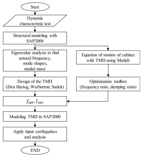
Figure 1.
Tuned mass damper (TMD) design and analysis process in this study.
Figure 2 shows the dimensions, external shape, and finite element model of the electrical cabinet that was used to confirm its acceleration response during an earthquake. The target cabinet in this study is the same as those used in NPPs. The dimensions of the electrical cabinet were 0.8 m × 0.8 m × 2.1 m and the total mass was 259 kg. The electrical cabinet was modeled while using beams and plates (see Figure 2c). The base of the electrical cabinet was restrained using eight connections. Table 1 lists the material properties of the electrical cabinet.
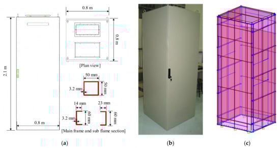
Figure 2.
Electrical cabinet model: (a) Dimensions of the electrical cabinet; (b) Prototype of the electrical cabinet; and, (c) Finite element model.

Table 1.
Material properties of the electrical cabinet.
2.2. Shaking Table Test of the Electrical Cabinet
In this study, a shaking table test was performed to identify the dynamic characteristics of the electrical cabinet. Figure 3a shows the test setup and sensor locations and Figure 3b shows the shaking table facility. The accelerometer was a 393B04 model [36] that could measure acceleration in the 5 g range in one direction. The dimensions of the shaking table were 1.0 m × 1.0 m in width and height, and it could be excited in the frequency range of 0.5–50 Hz, with an acceleration of 3 g for a 500 kg specimen (excitation force = 14.7 kN).
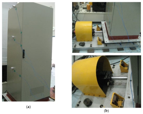
Figure 3.
Shaking table test of the electrical cabinet: (a) Cabinet and sensors; and, (b) Shaking table and servo motor.
Figure 4 shows the transfer function of the acceleration responses that were obtained from the shaking table test. Table 2 summarizes the dynamic test results. The damping ratio derived from the shaking table test was used to update the numerical model and for seismic analysis of the electrical cabinet in the SAP2000 software. In addition, the natural frequency derived from the shaking table test was used to verify the numerical model.
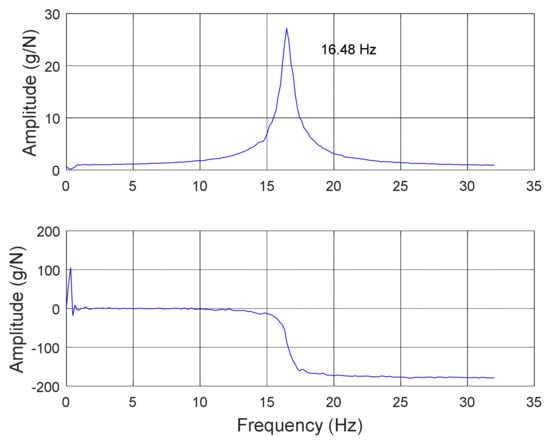
Figure 4.
Transfer function of the electrical cabinet obtained from shaking table test.
Table 2.
Results of shaking table test.
2.3. Eigenvalue Analysis
The dynamic properties of the electrical cabinet were derived from eigenvalue analysis while using SAP2000 software. One-hundred modes were calculated in the eigenvalue analysis. At this time, the modal participating mass ratios became about 95%. Figure 5 shows the first through third mode shapes of the electrical cabinet. In Figure 5a,b,d, the white dotted lines represent the vibrations of only the walls of the electrical cabinet. That is, only the third mode displays global behavior, while the remaining modes represent the local behavior. Therefore, the third mode was selected to be controlled by the TMD. The frequency for control mode in the numerical analysis was about 15.13 Hz and the modal mass was calculated while using the following equation:
where is the number of nodes, is the mass of the -th node, and is an eigenvector of the -th node of the -th mode. The maximum value of at the top of the electrical cabinet was normalized to 1. The calculated modal mass was 133 kg for the third mode. Reflecting on the results of the shaking table test, a structural damping of 2.16% was selected for the seismic analysis. Table 3 shows the dynamic properties of the electrical cabinet.
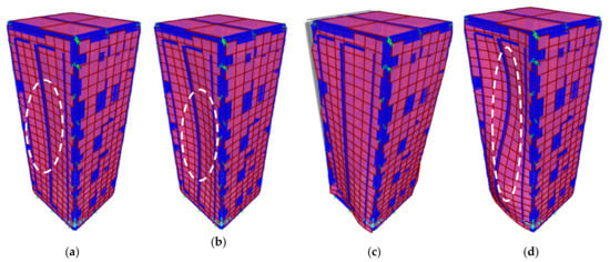
Figure 5.
Mode shapes of the electrical cabinet: (a) First mode (x-direction); (b) Second mode (x-direction); (c) Third mode (y-direction); and (d) Fourth mode (x-direction).
Table 3.
Dynamic properties of the electrical cabinet.
2.4. Optimum Design of TMD
The design variables of the TMD are functions of the mass ratio. Den Hartog [8], Warburton [9], and Sadek [37] proposed the optimum frequency ratios () and optimal damping ratios () of the TMD for random vibrations, which are expressed in Table 4.
Table 4.
Optimum parameters suggested for the TMD design.
Here, is the mass ratio of the TMD, is the optimal frequency ratio, and is the optimal damping ratio. in the Sadek equation is the damping ratio of the electrical cabinet.
In addition to the above three equations, the optimal TMD parameters were calculated while using an equation of motion with two degrees of freedom for an electrical cabinet with a TMD. Figure 6 shows a block diagram of the objective function of the optimization problem. “Plant” means the electrical cabinet with the TMD. “In” and “Out” refer to the seismic load and the response of the electrical cabinet, respectively. The optimization problem is defined as the problem of minimizing the frequency response function (FRF) by changing the input parameters and .
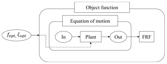
Figure 6.
Block diagram of the objective function.
The equation of motion of the electrical cabinet with the TMD subjected to an earthquake can be expressed as
where
where , , and are matrices of the mass, damping, and stiffness of the electrical cabinet system with the TMD, respectively; , , and are mass, damping, and stiffness of the electrical cabinet, respectively; , , and are the mass, damping, and stiffness of the TMD, respectively; is the ground acceleration; is the displacement of the electrical cabinet; and, is the displacement of the TMD. The stiffness of the electrical cabinet was calculated while using the third frequency and modal mass of the electrical cabinet in Table 3. The damping and stiffness of the electrical cabinet can be calculated using the following equations:
where , , and are the damping ratio (2.16%), natural frequency (15.13 Hz), and modal mass (133 kg) of the electrical cabinet, respectively. Therefore, the calculated stiffness and damping are 1.2 × 10⁶ N/m and 546 N∙s/m, respectively. Figure 7 shows the TMD that was installed above the electrical cabinet and the idealized two-degree-of-freedom model for the above equation of motion.
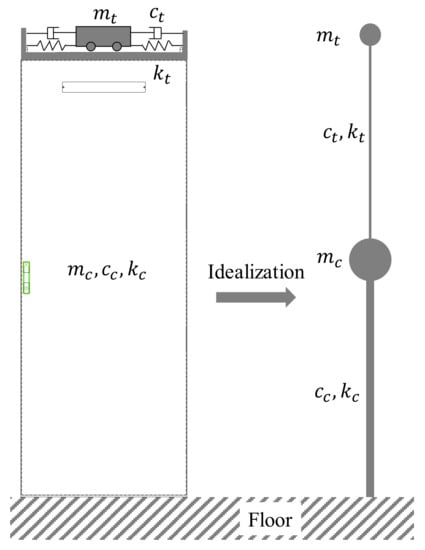
Figure 7.
TMD installation concept and idealization.
As shown in Table 4, the parameters of the TMD are the frequency and damping ratios, and these parameters were set as the boundary conditions for solving the optimization problem. The frequency ratio ranges from 0.6 to 1.3 and the damping ratio ranges from 1% to 30%.
A sinusoidal sweep wave was used as the ground acceleration in the equation of motion. The maximum acceleration magnitude of the sinusoidal sweep wave was 0.01 and the frequency range was 0.1–250 Hz. The objective function was defined as in Equation (7) to minimize the peak of the FRF for the input acceleration and the acceleration response of the electrical cabinet:
where is the FRF; and are the cross-spectra between the input and output and the auto spectra of the input and output, respectively; and, and are the input acceleration and acceleration response of the cabinet, respectively.
Figure 8 shows the FRFs before and after optimization obtained while using Equation (2) when the sinusoidal sweep wave was applied. Figure 9 presents the 3D plot of the FRF peaks, depending on the frequency and damping ratios. The red star in the figure represents the optimal point for minimizing the peak in the FRF. The optimum frequency and damping ratios are 0.874% and 18.9%, respectively. The numerical analysis of the equation of motion was simulated while using Matlab and Optimtool of MathWorks [38]. Table 5 shows the parameters of the TMD that were suggested by Den Hartog, Warburton, and Sadek and those of the proposed optimization method. Here, the damping ratio of the cabinet was identified by the experiment to 2.16% and the mass ratio of the TMD was set 7.5% to increase the cabinet’s target damping ratio to 12%.
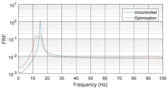
Figure 8.
Frequency response function (FRF) of electrical cabinet before and after optimization under sinusoidal sweep wave.
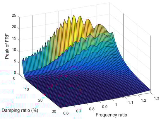
Figure 9.
FRF peak surface depending on TMD parameters.
Table 5.
Properties of TMDs designed while using optimum methods.
Multiple simulations are necessary through trial and error to obtain sufficient results, although the TMD is designed with the equations in Table 4. However, since the proposed optimization method already performs this execution error automatically in the optimization process, which reduces the time and effort of personnel.
2.5. Numerical Model of the Electrical Cabinet
Figure 10a,b show the numerical models of the electrical cabinet without and with the TMD. In Figure 10b, the green line in a dotted circle represents the TMD. The TMD and cabinet were modeled while using SAP2000 software. A two-point link was used to model the TMD. The initial point was attached to the top of the electrical cabinet. The mass of the TMD was added to the endpoint. The stiffness of the link, damping coefficient, and mass were applied while using the TMD design parameters in Table 5.
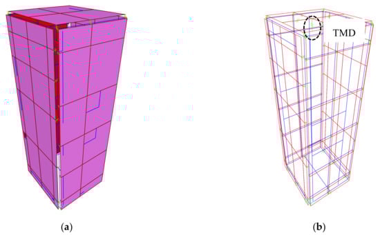
Figure 10.
Numerical models of electrical cabinet: (a) Without a TMD; and, (b) With a TMD.
3. Base Excitation
3.1. Sinusoidal Sweep Wave
The sinusoidal sweep wave was used to confirm the response properties of the electrical cabinet according to the frequency range and vibration control performance of the TMD. Figure 11 shows the time history of the sinusoidal sweep wave and its fast Fourier transform (FFT). The maximum acceleration magnitude of the sinusoidal sweep wave is 0.01 , and the frequency range is 0.1–250 Hz.
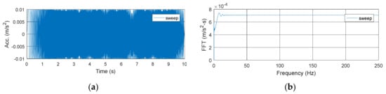
Figure 11.
Sinusoidal sweep wave and its fast Fourier transform (FFT): (a) Sweep wave; (b) FFT.
3.2. Floor Acceleration for Seismic Loads
Seven sets of floor accelerations were created that were compatible with the regulatory guide (RG) 1.60 design spectrum of 0.3 g PGA for seismic analysis of the electrical cabinet [39]. Figure 12 shows the seven generated response spectra and DRS.
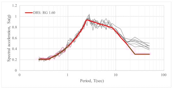
Figure 12.
Horizontal design response spectrum (DRS) of RG 1.60 spectrum (5% damping).
Seven sets of input floor accelerations were used to verify the vibration reduction performance and applicability of the TMD for the electrical cabinet. Figure 13, Figure 14, Figure 15, Figure 16, Figure 17, Figure 18 and Figure 19 show the time history and response spectrum of the floor acceleration for each of the seven seismic loads, and Table 6 summarizes the characteristics of each floor acceleration.
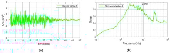
Figure 13.
Imperial Valley-2: (a) Time history; (b) Response spectrum.
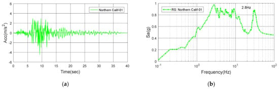
Figure 14.
Northern Calif-01: (a) Time history; (b) Response spectrum.
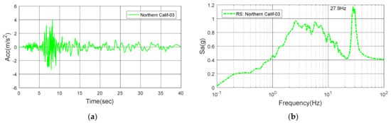
Figure 15.
Northern Calif-03: (a) Time history; (b) Response spectrum.
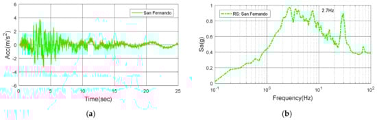
Figure 16.
San Fernando: (a) Time history; (b) Response spectrum.
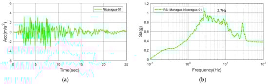
Figure 17.
Nicaragua-01: (a) Time history; (b) Response spectrum.

Figure 18.
Friuli: (a) Time history; (b) Response spectrum.
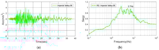
Figure 19.
Imperial Valley-06: (a) Time history; (b) Response spectrum.
Table 6.
Characteristics of seismic loads.
4. Results and Discussion
4.1. Acceleration Response of the Electrical Cabinet Under a Sinusoidal Sweep Wave
A sinusoidal sweep wave was used for the excitation of the electrical cabinet facility in this research for the following reasons:
- 1.
- to confirm the frequency characteristics of the electrical cabinet before and after the installation of the TMD, and
- 2.
- to investigate the reduction in the acceleration response.
Figure 20 shows the time history graph and response spectrum of the acceleration on the top of the electrical cabinet due to the sinusoidal sweep wave. The red dotted line represents the acceleration response of the electrical cabinet without the TMD. The cyan, blue, black, and magenta lines represent the acceleration responses of the electrical cabinet by the TMDs that are designed while using the Den Hartog, Warburton, and Sadek equations and proposed optimization, respectively. The maximum acceleration response of the electrical cabinet without the TMD is 0.92 m/s2, and those of the controlled acceleration peaks are 0.55–0.64 m/s2 (see Figure 20a). The rate of acceleration decrease due to TMD installation is 30–40%. The acceleration response of the electrical cabinet without the TMD shows a peak of 0.474 at about 15.0 Hz, but the peaks of the acceleration responses of the electrical cabinets with the TMDs show peaks of 0.272–0.299 (Figure 20b). The peak reduction rate of the response spectrum due to TMD installation is 37–43%, according to each design method. The vibration control effect of the electrical cabinet by the TMD was confirmed under the sinusoidal sweep load.
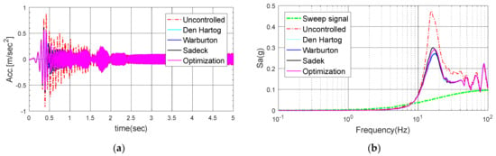
Figure 20.
Acceleration response at the top of the electrical cabinet when subjected to a sinusoidal sweep wave: (a) Time history; (b) Response spectrum.
4.2. Acceleration Responses of Electrical Cabinet Subjected to Earthquakes
Figure 21a, Figure 22a, Figure 23a, Figure 24a, Figure 25a, Figure 26a and Figure 27a show the envelopes of the acceleration at the top of the electrical cabinet, with and without a TMD. Here, the envelope plots were adopted to show several time histories. The red dotted line represents the acceleration response of the electrical cabinet without the TMD. The cyan, blue, black, and magenta lines represent the acceleration responses of the electrical cabinets with TMDs that are designed while using the Den Hartog, Warburton, and Sadek methods and the proposed optimization.
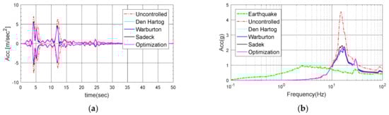
Figure 21.
Response of the electrical cabinet subjected to Imperial Valley-2: (a) Time history; (b) Response spectrum.
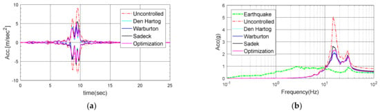
Figure 22.
Response of the electrical cabinet subjected to Northern Calif-01: (a) Time history; (b) Response spectrum.
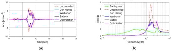
Figure 23.
Response of the electrical cabinet subjected to Northern Calif-03: (a) Time history; (b) Response spectrum.
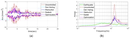
Figure 24.
Response of the electrical cabinet subjected to San Fernando: (a) Time history; (b) Response spectrum.
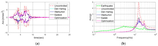
Figure 25.
Response of the electrical cabinet subjected to Nicaragua-01: (a) Time history; (b) Response spectrum.
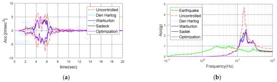
Figure 26.
Response of the electrical cabinet subjected to Friuli: (a) Time history; (b) Response spectrum.
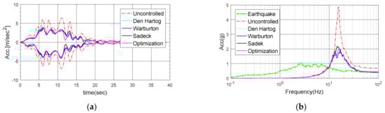
Figure 27.
Response of the electrical cabinet subjected to Imperial Valley-06: (a) Time history; (b) Response spectrum.
In Figure 21a, the maximum acceleration response of the electrical cabinet with the TMD (Warburton) in the Imperial Valley-2 earthquake case decreases from 7.64 to 5.17 m/s2 and the maximum rate of decrease is about 32%. Figure 22a shows the maximum acceleration response of the electrical cabinet due to the Northern Calif-01 earthquake. The maximum acceleration decreases from 7.82 to 5.19 m/s2 and the maximum rate of decrease is about 33%. In Figure 23a, the maximum acceleration response of the electrical cabinet with the TMD (optimization) in the Northern Calif-03 earthquake case decreases from 7.67 to 4.79 m/s2, and the maximum decrease rate is about 37%. In the case of the San Fernando earthquake, the maximum acceleration response decreases from 8.42 to 5.13 m/s2 and the rate of decrease is about 39% (see Figure 24a). Figure 25a shows the maximum acceleration response due to the Nicaragua-01 earthquake. Here, the maximum acceleration decreases from 6.75 to 3.79 m/s2 and the maximum rate of decrease is about 44%. Figure 26a shows the maximum acceleration response in the Friuli earthquake case. The maximum acceleration decreases from 7.29 to 4.67 m/s2 and the maximum rate of decrease is about 36%. In the last earthquake, the Imperial Valley-06 earthquake, the maximum acceleration without control is 6.55 m/s2, and the maximum acceleration with the TMD is 3.95 m/s2 (see Figure 27a). The rate of decrease is about 40%. In the acceleration time history results for the TMD, the average reduction rate is 35.5% and the standard deviation is 4.4%.
Figure 21b, Figure 22b, Figure 23b, Figure 24b, Figure 25b, Figure 26b and Figure 27b show the response spectrum of the acceleration at the top of the electrical cabinet, with and without TMD. The response spectrum of the floor acceleration (green line) is also presented for comparison with the acceleration response characteristics of the electrical cabinet. In each acceleration response spectrum, acceleration amplification is evident at the frequency that corresponds to the third mode of the electrical cabinet for each input floor acceleration. Figure 21b shows the response spectrum of the electrical cabinet in the Imperial Valley-2 earthquake case. It can be seen that the response spectrum is significantly reduced between 10 and 20 Hz by the TMD. The peak of the response spectrum is decreased from 4.54 to 2.08, and the rate of decrease is approximately 54%. Figure 22b shows the peak of the response spectrum that is caused by the Northern Calif-01 earthquake. Here, the peak of the response spectrum decreases from 5.06 to 2.09 , and the maximum rate of decrease is about 59%. In Figure 23b, the peak of the response spectrum with the TMD (optimization) in the Northern Calif-03 earthquake case decreases from 4.70 to 2.20 , and the maximum rate of decrease is approximately 53%. Figure 24b shows the peak of the response spectrum that is caused by the San Fernando earthquake, and the maximum rate of decrease is about 61%. In the case of the Nicaragua-01 earthquake, the response spectrum is reduced by about 63% (see Figure 25b). Figure 26b and Figure 27b show the response spectrum of the electrical cabinet that is caused by the Friuli and Imperial Valley-06 earthquakes, and the rates of decrease are approximately 50% and 63%, respectively. The average reduction rate is 54.1% and the standard deviation is 5.0%. It was confirmed that the TMD effectively reduced the response spectrum amplification.
Table 7 shows the maximum accelerations of the uncontrolled cabinet and the electrical cabinets controlled by the TMDs designed while using each equation. The rate of decrease of the maximum acceleration is also presented. The equation of Den Hartog produced the greatest control effect in the Imperial Valley-06 earthquake case, and the equation of Sadek showed the greatest reduction effect in the Friuli earthquake case. A good control effect was observed with the TMD designed while using the equation of Warburton, which showed the maximum rate of decrease in the Imperial Valley-2, Northern Calif-01, San Fernando, and Nicaragua-01 earthquake cases. The proposed optimization method provided the best vibration reduction effect in the Northern Calif-03 earthquake case.
Table 7.
Maximum acceleration in each earthquake case.
Table 8 shows the peak spectral accelerations of the uncontrolled and controlled electrical cabinets. In the peak spectral acceleration, the vibration reduction effect was the greatest for almost all of the earthquakes in the Warburton equation case. The equation of Den Hartog produced the greatest control effect (62.9%) in the Imperial Valley-06 earthquake case, while the proposed optimization method yielded the best vibration reduction effect (53.1%) in the Northern Calif-03 earthquake case.
Table 8.
Peak spectral acceleration for each earthquake.
4.3. Comparison of Control Results
Figure 28 shows a bar graph of the amplification factor (AF) for each base excitation in the electrical cabinet that was obtained using Equation (8):
where and are the peaks of the response spectrum of the electrical cabinet and the base excitation, respectively. In the bar graph, each earthquake corresponds to the earthquake sequence in Table 8. The blue bar represents the AF of the uncontrolled cabinet. The red bar represents the AF of the electrical cabinet that is controlled by the TMD. The TMD used here was designed with the proposed optimization method. The maximum AF was 6.5 in the San Fernando earthquake case (EQ4) and decreased to 3.1 when controlled by the TMD.
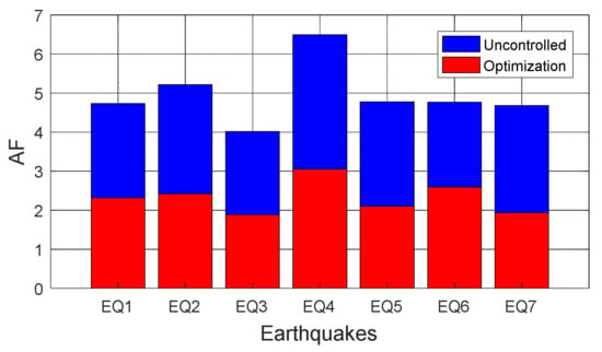
Figure 28.
Amplification factor (AF) due to seismic loads of the electrical cabinet with and without a TMD.
Table 9 shows the AF and rate of decrease. The TMD reduced the AF for all seven earthquake loads from 1.9 to 3.1 when designed using the proposed optimization method. The average reduction rate is 53% and the standard deviation is 3.8%. Time–frequency analysis of the San Fernando and Imperial Valley-06 earthquakes was performed, and Figure 29 and Figure 30, respectively, show the results. Figure 29a and Figure 30a depict the uncontrolled and controlled accelerations at the top of the electrical cabinet. The controlled response here is the acceleration of the electrical cabinet with the TMD designed by optimization. Figure 29b,c show the results of time–frequency analysis before and after control in the San Fernando earthquake case.
Table 9.
AF and rate of decrease due to seismic loading of the electrical cabinet with and without a TMD.
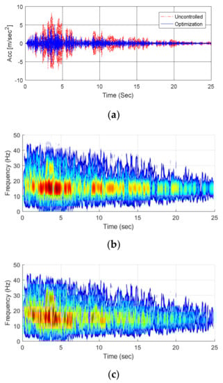
Figure 29.
Results of time–frequency analysis of the electrical cabinet subjected to San Fernando: (a) Time history; (b) Uncontrolled response; and, (c) Controlled response.
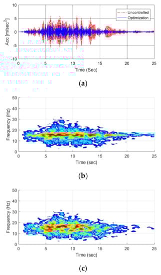
Figure 30.
Results of time–frequency analysis of the electrical cabinet subjected to Imperial Valley-06: (a) Time history; (b) Uncontrolled response; and, (c) Controlled response.
Figure 30b,c presents the results of the time–frequency analysis before and after control in the Imperial Valley-06 earthquake case. Finally, the time–frequency analysis results for the TMD that was designed as an optimization method were compared with the uncontrolled results. It can be seen that the dark red at 15 Hz turns pale during the TMD operation. The numerical results show that the TMD can sufficiently reduce the vibration acceleration of the electrical cabinet.
5. Conclusions
In this study, TMDs were applied to reduce the vibration acceleration of the electrical equipment inside an NPP subjected to earthquakes. A shaking table test was performed, and the natural frequency and damping ratio of the cabinet were extracted, to confirm the dynamic characteristics of the electrical cabinet. TMDs were designed while using an optimization method and the equations that were proposed by Den Hartog, Warburton, and Sadek, together with the results of eigenvalue analysis of the target cabinet. Electrical cabinets with and without TMDs were modeled while using SAP2000 software. A sinusoidal sweep wave was used as an input motion at the base to identify the vibration characteristics of the electrical cabinet over a wide frequency range. The seismic loads of seven input floor accelerations adjusted to meet the DRS were used in this study to confirm the control effects of the TMDs in earthquakes. The acceleration responses before and after the control of the electrical cabinet while using the TMDs were compared using the time and frequency domains. The acceleration reduction performances of the TMDs designed using each optimization method were compared based on the response spectrum and AF. The key observations and findings of this research are as follows:
- (1)
- The electrical cabinets with TMDs confirmed that the vibration acceleration due to seismic loading was reduced significantly more, and the vibration control effects resulting from using the TMD optimization design method differed slightly, but not significantly.
- (2)
- The seismic response of the uncontrolled electrical cabinet was reduced by more than 30% by the TMD that was designed through the optimization technique.
- (3)
- The AFs of the electrical cabinets subjected to seismic loads were calculated. The average AF reduction rate was 53% and the standard deviation was 3.8%.
- (4)
- Finally, the numerical analysis verified that TMDs could be effectively applied to the electrical cabinets inside NPPs under earthquakes. This study numerically demonstrates that TMDs can be considered to be useful for improving the seismic performance of the electrical equipment inside NPPs.
TMD can be considered as an effective way to improve the seismic performance of the cabinet if the electrical cabinet of the existing NPP fails to meet the required seismic demand. Further experimental verification of electrical cabinets with TMDs and evaluation of seismic performance are also considered to be necessary.
Author Contributions
Conceptualization, S.G.C., D.S. and S.C.; methodology, S.C. and D.S.; software, S.C.; validation, S.G.C.; writing—original draft preparation, S.C.; writing—review and editing, S.G.C. and D.S. All the authors approved the final manuscript. All authors have read and agreed to the published version of the manuscript.
Funding
This research was funded by the Ministry of Trade, Industry & Energy (MOTIE) of the Republic of Korea grant number no 20161520101270.
Acknowledgments
This work was supported by the Energy Technology Development Program of the Korea Institute of Energy Technology Evaluation and Planning (KETEP) grant financial resource from the Ministry of Trade, Industry & Energy, Republic of Korea (No. 20161520101270).
Conflicts of Interest
The authors declare no conflict of interest.
References
- Tran, T.T.; Cao, A.T.; Nguyen, T.H.X.; Kim, D. Fragility assessment for electric cabinet in nuclear power plant using response surface methodology. Nucl. Eng. Technol. 2019, 51, 894–903. [Google Scholar] [CrossRef]
- Tran, T.T.; Kim, D. Uncertainty quantification for nonlinear seismic analysis of cabinet facility in nuclear power plants. Nucl. Eng. Des. 2019, 355, 110309. [Google Scholar] [CrossRef]
- McFarlane, J.P. The Seismic Assessment of British Energy’s Nuclear Power Stations and Some Pragmatic Solutions to Seismic Modifications. In Proceedings of the Workshop on the Seismic Re-Evaluation of All Nuclear Facilities, Ispra, Italy, 26–27 March 2001. [Google Scholar]
- Kim, D.K.; Kim, W.B.; Suh, Y.P.; Moon, D.S.; Kim, J.Y. Seismic Performance Evaluation for MCR of Nuclear Power Plant Isolated by FPS. J. Proc. Earthq. Eng. Soc. Korea Conf. 2003, 453–460. [Google Scholar]
- Kim, W.B.; Lee, K.; Kim, G.H. Application of friction pendulum system to the main control room of a nuclear power plant. Can. J. Civ. Eng. 2009, 36, 63–72. [Google Scholar] [CrossRef]
- Jeon, B.G.; Chang, S.J.; Kim, S.W.; Kim, N.S. Base isolation performance of a cone-type friction pendulum bearing system. Struct. Eng. Mech. 2015, 53, 227–248. [Google Scholar] [CrossRef]
- Cho, S.G.; Hwang, K.T.; Park, W.K.; So, G.H. Vibration Response Reduction Effects of Isolation Table System with LM Guide. J. Proc. Earthq. Eng. Soc. Korea Conf. 2013, 131–134. [Google Scholar]
- Den Hartog, J.P. Mechanical Vibrations, 4th ed.; McGraw-Hill: New York, NY, USA, 1956. [Google Scholar]
- Warburton, G.B. Optimum Absorber Parameters for Various Combinations of Response and Excitation Parameters. Earthq. Eng. Struct. Dyn. 1982, 10, 381–401. [Google Scholar] [CrossRef]
- Kwok, K.C.S.; Samali, B. Performance of tuned mass dampers under wind loads. Eng. Struct. 1995, 17, 655–667. [Google Scholar] [CrossRef]
- Elias, S.; Matsagar, V. Distributed multiple tuned mass dampers for wind vibration response control of high-rise building. J. Eng. 2014, 2014, 1–11. [Google Scholar] [CrossRef]
- Elias, S.; Matsagar, V. Research developments in vibration control of structures using passive tuned mass dampers. Annu. Rev. Control 2017, 44, 129–156. [Google Scholar] [CrossRef]
- Giaralis, A.; Petrini, F. Optimum design of the tuned mass-damper-inerter for serviceability limit state performance in wind-excited tall buildings. Procedia Eng. 2017, 199, 1773–1778. [Google Scholar] [CrossRef]
- Elias, S.; Matsagar, V. Wind response control of tall buildings with a tuned mass damper. J. Build. Eng. 2018, 15, 51–60. [Google Scholar] [CrossRef]
- Abdulsalam, I.; Al-Janani, M.; Al-Taweel, M.G. Optimum design of tuned mass damper systems for seismic structures. In Proceedings of the 7th International Conference on Earthquake Resistant Engineering Structures, WIT Press, Limassol, Cyprus, 11–13 May 2009; Volume 104, pp. 175–184. [Google Scholar] [CrossRef]
- Domizio, M.; Ambrosini, D.; Oscar, C. Performance of tuned mass damper against structural collapse due to near fault earthquakes. J. Sound Vib. 2015, 336, 32–45. [Google Scholar] [CrossRef]
- Rahman, M.S.; Chang, S.; Kim, D. Multiple wall dampers for multi-mode vibration control of building structures under earthquake excitation. Struct. Eng. Mech. 2017, 63, 537–549. [Google Scholar]
- Salvi, J.; Pioldi, F.; Rizzi, E. Optimum Tuned Mass Dampers under seismic Soil-Structure Interaction. Soil Dyn. Earthq. Eng. 2018, 114, 576–597. [Google Scholar] [CrossRef]
- Elias, S.; Matsagar, V.; Datta, T.K. Distributed tuned mass dampers for multi-mode control of benchmark building under seismic excitations. J. Earthq. Eng. 2019, 23, 1137–1172. [Google Scholar] [CrossRef]
- Elias, S.; Matsagar, V.; Datta, T.K. Dynamic response control of a wind-excited tall building with distributed multiple tuned mass dampers. Int. J. Struct. Stab. Dyn. 2019, 19, 1950059. [Google Scholar] [CrossRef]
- Li, B.; Dai, K.; Li, H.; Li, B.; Tesfamariam, S. Optimum design of a non-conventional multiple tuned mass damper for a complex power plant structure. Struct. Infrastruct. Eng. 2019, 15, 954–964. [Google Scholar] [CrossRef]
- Zhou, S.; Jean-Mistral, C.; Chesne, S. Influence of inerters on the vibration control effect of series double tuned mass dampers: Two layouts and analytical study. Struct. Control Health Monit. 2019, 26, e2414. [Google Scholar] [CrossRef]
- Rahmani, H.R.; Konke, C. Seismic control of tall buildings using distributed multiple tuned mass dampers. Adv. Civ. Eng. 2019, 2019, 6480384. [Google Scholar] [CrossRef]
- Vellar, L.S.; Ontiveros-Perez, S.P.; Fadel Miguel, L.F.; Fadel Miguel, L.F. Robust Optimum Design of Multiple Tuned Mass Dampers for Vibration Control in Buildings Subjected to Seismic Excitation. Shock Vib. 2019, 2019, 9273714. [Google Scholar] [CrossRef]
- Lu, Z.; Li, K.; Ouyang, Y.; Shan, J. Performance-based optimal design of tuned impact damper for seismically excited nonlinear building. Eng. Struct. 2018, 160, 314–327. [Google Scholar] [CrossRef]
- Elias, S.; Matsagar, V. Seismic vulnerability of non-linear building with distributed multiple tuned vibration absorbers. Struct. Infrastruct. Eng. 2019, 15, 1103–1118. [Google Scholar] [CrossRef]
- Nakai, T.; Kurino, H.; Yaguchi, T.; Kano, N. Control effect of large tuned mass damper used for seismic retrofitting of existing high-rise building. Jpn. Archit. Rev. 2019, 2, 269–286. [Google Scholar] [CrossRef]
- Chang, S.; Sun, W.; Cho, S.G.; Kim, D. Vibration Control of Nuclear Power Plant Piping System Using Stockbridge Damper under Earthquakes. Sci. Technol. Nucl. Install. 2016, 2016, 5014093. [Google Scholar] [CrossRef]
- Jiang, J.; Zhang, P.; Patil, D.; Li, H.N.; Song, G. Experimental studies on the effectiveness and robustness of a pounding tuned mass damper for vibration suppression of a submerged cylindrical pipe. Struct. Control Health Monit. 2017, 24, e2027. [Google Scholar] [CrossRef]
- Tan, J.; Ho, M.; Chun, S.; Zhang, P.; Jiang, J. Experimental Study on Vibration Control of Suspended Piping System by Single-Sided Pounding Tuned Mass Damper. Appl. Sci. 2019, 9, 285. [Google Scholar] [CrossRef]
- Jiang, J.; Ho, S.C.M.; Markle, N.J.; Wang, N.; Song, G. Design and control performance of a frictional tuned mass damper with bearing-shaft assemblies. J. Vib. Control 2019, 25, 1812–1822. [Google Scholar] [CrossRef]
- Kwag, S.; Kwak, J.; Lee, H.; Oh, J.; Koo, G.H. Enhancement in the Seismic Performance of a Nuclear Piping System using Multiple Tuned Mass Dampers. Energies 2019, 12, 2077. [Google Scholar] [CrossRef]
- Fabrizio, C.; de Leo, A.M.; Di Egidio, A. Tuned mass damper and base isolation: A unitary approach for the seismic protection of conventional frame structures. J. Eng. Mech. 2019, 145, 04019011. [Google Scholar] [CrossRef]
- Computers and Structures Inc. CSI Analysis Reference Manual for SAP2000; Computer and Structures Inc.: Berkley, CA, USA, 2010. [Google Scholar]
- Pacific Earthquake Engineering Research Center. Available online: https://ngawest2.berkeley.edu/site (accessed on 11 October 2019).
- SEISMIC ICP® ACCELEROMETER. Available online: https://www.pcb.com/contentstore/docs/PCB_Corporate/Vibration/Products/Specsheets/393B04_G.pdf (accessed on 11 December 2019).
- Sadek, F.; Mohraz, B.; Taylor, A.W.; Chung, R.M. A method of estimating the parameters of tuned mass dampers for seismic applications. Earthq. Eng. Sturct. Dyn. 1997, 26, 617–635. [Google Scholar] [CrossRef]
- The Math Works Inc. Matlab 2016; The Math Works Inc.: Natick, MA, USA, 2016. [Google Scholar]
- United States Nuclear Regulatory Commission (USNRC). Design Response Spectra for Seismic Design of Nuclear Power Plants, Regulatory Guide; United States Nuclear Regulatory Commission: Rockville, MD, USA, 2014. [Google Scholar]


© 2020 by the authors. Licensee MDPI, Basel, Switzerland. This article is an open access article distributed under the terms and conditions of the Creative Commons Attribution (CC BY) license (http://creativecommons.org/licenses/by/4.0/).