Assessment of Simulated Solar Irradiance on Days of High Intermittency Using WRF-Solar


Abstract
1. Introduction
2. Materials and Methods
2.1. Surface Observations
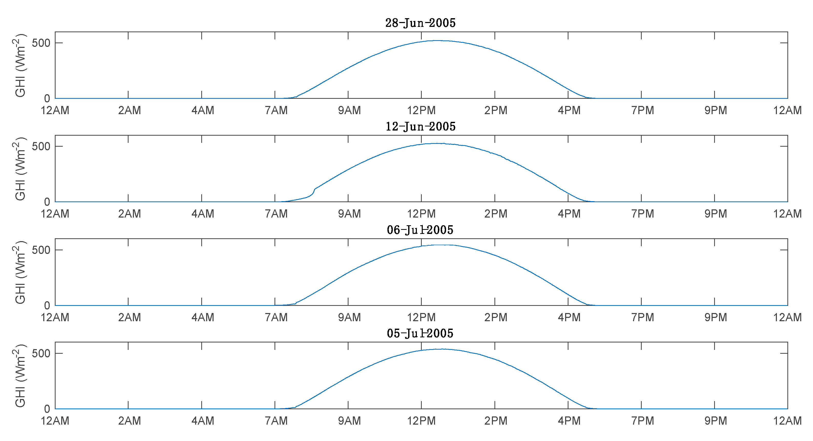
2.2. Observed Cases
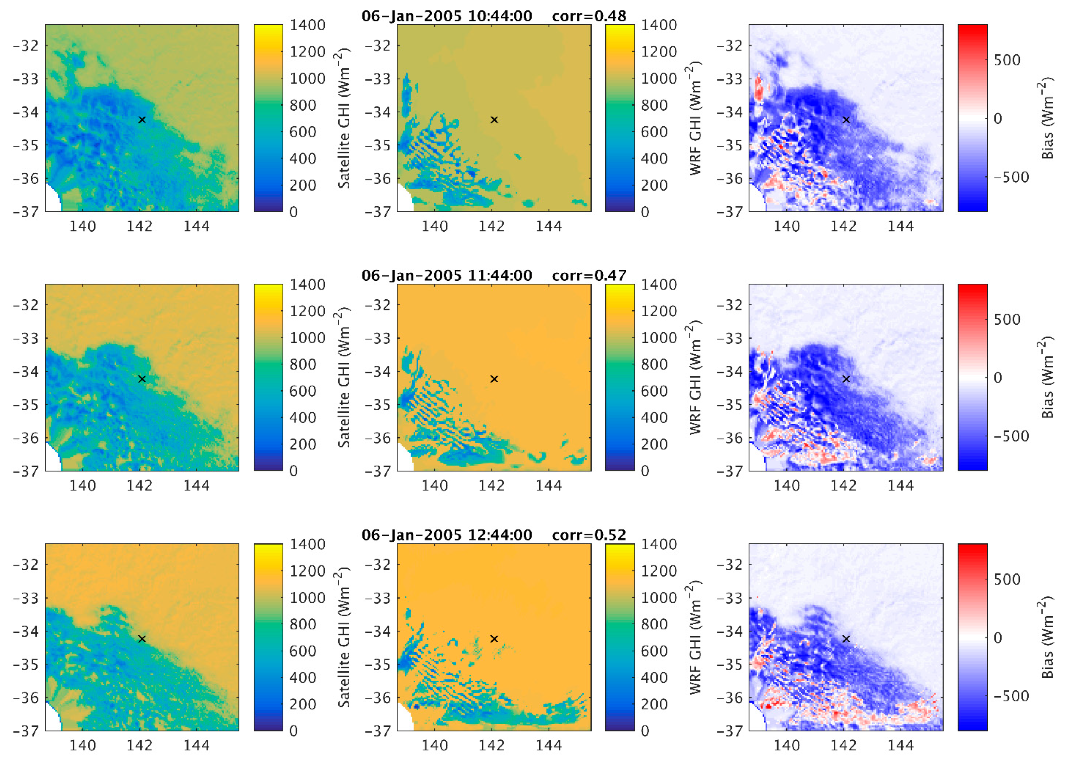
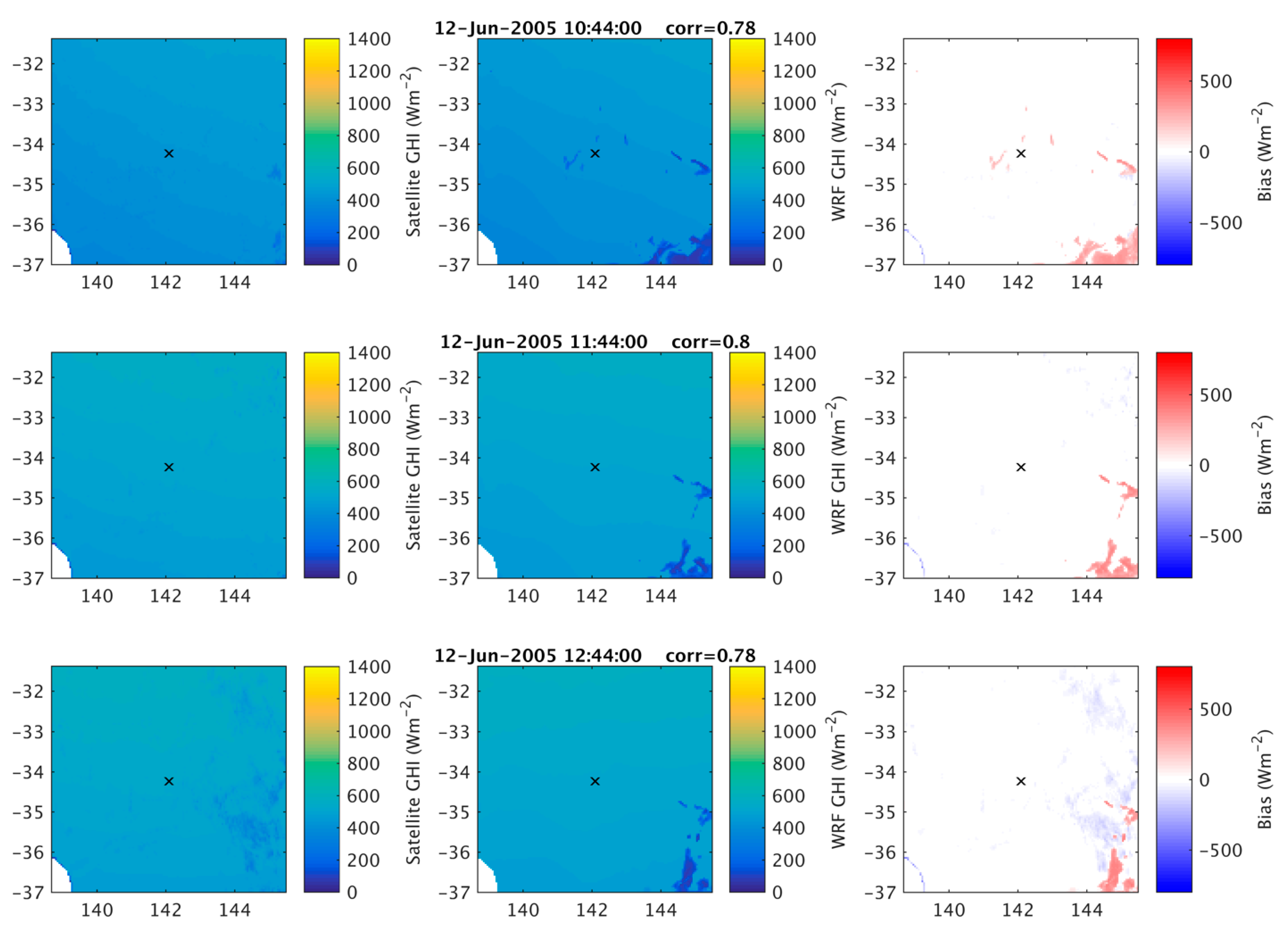
2.3. Satellite Data
2.4. Reanalysis Forcing Data
2.5. Model Setup
2.6. Evaluation Procedure
3. Results
3.1. Evaluating Solar Irradiance Variables
3.2. Evaluating Surface Variables
3.3. Bias Exploration
3.4. Evaluation of Long-Term Simulations
4. Discussion
5. Conclusions
Author Contributions
Funding
Acknowledgments
Conflicts of Interest
References
- Hayat, M.B.; Ali, D.; Monyake, K.C.; Alagha, L.; Ahmed, N. Solar energy—A look into power generation, challenges, and a solar-powered future. Int. J. Energy Res. 2019, 43, 1049–1067. [Google Scholar] [CrossRef]
- Kannan, N.; Vakeesan, D. Solar energy for future world:—A review. Renew. Sust. Energy Rev. 2016, 62, 1092–1105. [Google Scholar] [CrossRef]
- Kabir, E.; Kumar, P.; Kumar, S.; Adelodun, A.A.; Kim, K.H. Solar energy: Potential and future prospects. Renew. Sust. Energy Rev. 2018, 82, 894–900. [Google Scholar] [CrossRef]
- Stefferud, K.; Kleissl, J.; Schoene, J. Solar forecasting and variability analyses using sky camera cloud detection & motion vectors. In Proceedings of the IEEE Power and Energy Society General Meeting, San Diego, CA, USA, 22–26 July 2012; pp. 1–6. [Google Scholar]
- Prasad, A.A.; Taylor, R.A.; Kay, M. Assessment of solar and wind resource synergy in Australia. Appl. Energy 2017, 190, 354–367. [Google Scholar] [CrossRef]
- Garcia, S.G.; Trautmann, T.; Venema, V. Reduction of radiation biases by incorporating the missing cloud variability by means of downscaling techniques: A study using the 3-D MoCaRT model. Atmos. Meas. Tech. 2012, 5, 2261–2276. [Google Scholar] [CrossRef]
- Nunez, M.; Fienberg, K.; Kuchinke, C. Temporal structure of the solar radiation field in cloudy conditions: Are retrievals of hourly averages from space possible? J. Appl. Meteorol. 2005, 44, 167–178. [Google Scholar] [CrossRef]
- Madhavan, B.L.; Deneke, H.; Witthuhn, J.; Macke, A. Multiresolution analysis of the spatiotemporal variability in global radiation observed by a dense network of 99 pyranometers. Atmos. Chem. Phys. 2017, 17, 3317–3338. [Google Scholar] [CrossRef]
- Law, E.W.; Prasad, A.A.; Kay, M.; Taylor, R.A. Direct normal irradiance forecasting and its application to concentrated solar thermal output forecasting—A review. Sol. Energy 2014, 108, 287–307. [Google Scholar] [CrossRef]
- Law, E.W.; Kay, M.; Taylor, R.A. Evaluating the benefits of using short-term direct normal irradiance forecasts to operate a concentrated solar thermal plant. Sol. Energy 2016, 140, 93–108. [Google Scholar] [CrossRef]
- Elliston, B.; MacGill, I. The potential role of forecasting for integrating solar generation into the Australian national electricity market. In Proceedings of the Solar 2010, the 48th AuSES Annual Conference, Canberra, Australia, 1–3 December 2010; p. 11. [Google Scholar]
- Bony, S.; Stevens, B.; Frierson, D.M.W.; Jakob, C.; Kageyama, M.; Pincus, R.; Shepherd, T.G.; Sherwood, S.C.; Siebesma, A.P.; Sobel, A.H.; et al. Clouds, circulation and climate sensitivity. Nat. Geosci. 2015, 8, 261–268. [Google Scholar] [CrossRef]
- Stevens, B.; Bony, S. What are climate models missing? Science 2013, 340, 1053–1054. [Google Scholar] [CrossRef] [PubMed]
- Sherwood, S.C.; Alexander, M.J.; Brown, A.R.; McFarlane, N.A.; Gerber, E.P.; Feingold, G.; Scaife, A.A.; Grabowski, W.W. Climate processes: Clouds, aerosols and dynamics. In Climate Science for Serving Society; Springer: Berlin, Germany, 2013. [Google Scholar]
- Birch, C.E.; Marsham, J.H.; Parker, D.J.; Taylor, C.M. The scale dependence and structure of convergence fields preceding the initiation of deep convection. Geophys. Res. Lett. 2014. [Google Scholar] [CrossRef]
- Yin, J.; Porporato, A. Diurnal cloud cycle biases in climate models. Nat. Commun. 2017, 8. [Google Scholar] [CrossRef] [PubMed]
- Bae, S.Y.; Hong, S.-Y.; Lim, K.-S.S. Coupling WRF double-moment 6-class microphysics schemes to RRTMG radiation scheme in weather research forecasting model. Adv. Meteorol. 2016, 2016, 11. [Google Scholar] [CrossRef]
- Thompson, G.; Tewari, M.; Ikeda, K.; Tessendorf, S.; Weeks, C.; Otkin, J.; Kong, F.Y. Explicitly-coupled cloud physics and radiation parameterizations and subsequent evaluation in WRF high-resolution convective forecasts. Atmos. Res. 2016, 168, 92–104. [Google Scholar] [CrossRef]
- Stensrud, D.J. Parameterization Schemes: Keys to Understanding Numerical Weather Prediction Models; Cambridge University Press: Cambridge, UK, 2009; p. 449. [Google Scholar]
- Haupt, S.E.; Jiménez, P.A.; Lee, J.A.; Kosović, B. Renewable Energy Forecasting; Woodhead Publishing: Sawston, UK; Cambridge, UK, 2017; pp. 3–28. [Google Scholar]
- Song, S.W.; Mapes, B. Interpretations of systematic errors in the NCEP Climate Forecast System at lead times of 2, 4, 8,..., 256 days. J. Adv. Model. Earth Sy. 2012, 4. [Google Scholar] [CrossRef]
- Holtslag, A.A.M.; Svensson, G.; Baas, P.; Basu, S.; Beare, B.; Beljaars, A.C.M.; Bosveld, F.C.; Cuxart, J.; Lindvall, J.; Steeneveld, G.J.; et al. Stable atmospheric boundary layers and diurnal cycles challenges for weather and climate models. Bull. Am. Meteorol. Soc. 2013, 94, 1691–1706. [Google Scholar] [CrossRef]
- Dehghan, A.; Prasad, A.A.; Sherwood, S.C.; Kay, M. Evaluation and improvement of TAPM in estimating solar irradiance in Eastern Australia. Sol. Energy 2014, 107, 668–680. [Google Scholar] [CrossRef]
- Gregory, P.A.; Rikus, L.J. Validation of the bureau of meteorology’s global, diffuse, and direct solar exposure forecasts using the ACCESS numerical weather prediction systems. J. Appl. Meteorol. Clim. 2016, 55, 595–619. [Google Scholar] [CrossRef]
- Gregory, P.A.; Rikus, L.J.; Kepert, J.D. Testing and diagnosing the ability of the bureau of meteorology’s numerical weather prediction systems to support prediction of solar energy production. J. Appl. Meteorol. Clim. 2012, 51, 1577–1601. [Google Scholar] [CrossRef]
- Huang, J.; Thatcher, M. Assessing the value of simulated regional weather variability in solar forecasting using numerical weather prediction. Sol. Energy 2017, 144, 529–539. [Google Scholar] [CrossRef]
- Troccoli, A.; Morcrette, J.J. Skill of direct solar radiation predicted by the ECMWF global atmospheric model over Australia. J. Appl. Meteorol. Clim. 2014, 53, 2571–2588. [Google Scholar] [CrossRef]
- Lorenz, E.; Kuhnert, J.; Heinemann, D.; Nielsen, K.P.; Remund, J.; Muller, S.C. Comparison of global horizontal irradiance forecasts based on numerical weather prediction models with different spatio-temporal resolutions. Prog. Photovolt. 2016, 24, 1626–1640. [Google Scholar] [CrossRef]
- Perez, R.; Lorenz, E.; Pelland, S.; Beauharnois, M.; Van Knowe, G.; Hemker, K.; Heinemann, D.; Remund, J.; Muller, S.C.; Traunmuller, W.; et al. Comparison of numerical weather prediction solar irradiance forecasts in the US, Canada and Europe. Sol. Energy 2013, 94, 305–326. [Google Scholar] [CrossRef]
- Ruiz-Arias, J.A.; Dudhia, J.; Santos-Alamillos, F.J.; Pozo-Vazquez, D. Surface clear-sky shortwave radiative closure intercomparisons in the weather research and forecasting model. J. Geophys. Res.Atmos. 2013, 118, 9901–9913. [Google Scholar] [CrossRef]
- Xie, Y.; Sengupta, M.; Dudhia, J. A fast all-sky radiation model for solar applications (FARMS): Algorithm and performance evaluation. Sol. Energy 2016, 135, 435–445. [Google Scholar] [CrossRef]
- Ruiz-Arias, J.A.; Dudhia, J.; Gueymard, C.A. A simple parameterization of the short-wave aerosol optical properties for surface direct and diffuse irradiances assessment in a numerical weather model. Geosci. Model. Dev. 2014, 7, 1159–1174. [Google Scholar] [CrossRef]
- Thompson, G.; Eidhammer, T. A study of aerosol impacts on clouds and precipitation development in a large winter cyclone. J. Atmos. Sci. 2014, 71, 3636–3658. [Google Scholar] [CrossRef]
- Deng, A.; Gaudet, B.; Dudhia, J.; Alapaty, K. Implementation and evaluation of a new shallow convection scheme in WRF. In Proceedings of the 26th Conference on Weather Analysis and Forecasting/22nd Conference on Numerical Weather Prediction, Atlanta, GA, USA, 2–6 February 2014. [Google Scholar]
- Skamarock, W.C.; Klemp, J.B.; Dudhia, J.; Gill, D.O.; Barker, D.M.; Duda, M.G.; Huang, X.Y.; Wang, W.; Powers, J.G. A description of the advanced research WRF Version 3. Citeseer 2008. [Google Scholar]
- Jimenez, P.A.; Hacker, J.P.; Dudhia, J.; Haupt, S.E.; Ruiz-Arias, J.A.; Gueymard, C.A.; Thompson, G.; Eidhammer, T.; Deng, A.J. WRF-solar description and clear-sky assessment of an augmented NWP model for solar power prediction. Bull. Am. Meteorol. Soc. 2016, 97, 1249–1264. [Google Scholar] [CrossRef]
- Jiménez, P.A.; Alessandrini, S.; Haupt, S.E.; Deng, A.; Kosovic, B.; Lee, J.A.; Delle Monache, L. The role of unresolved clouds on short-range global horizontal irradiance predictability. Res. Appl. Lab. Natl. Cent. Atmos. Res. Boulder Colo. 2016, 144, 3099–3107. [Google Scholar] [CrossRef]
- Lee, J.A.; Haupt, S.E.; Jimenez, P.A.; Rogers, M.A.; Miller, S.D.; McCandless, T.C. Solar irradiance nowcasting case studies near sacramento. J. Appl. Meteorol. Clim. 2017, 56, 85–108. [Google Scholar] [CrossRef]
- Reikard, G.; Haupt, S.E.; Jensen, T. Forecasting ground-level irradiance over short horizons: Time series, meteorological, and time-varying parameter models. Renew. Energy 2017, 112, 474–485. [Google Scholar] [CrossRef]
- Haupt, S.E.; Kosovic, B.; Jensen, T.; Lazo, J.K.; Lee, J.A.; Jimenez, P.A.; Cowie, J.; Wiener, G.; McCandless, T.C.; Rogers, M.; et al. Building the Sun4cast system improvements in solar power forecasting. Bull. Am. Meteorol. Soc. 2018, 99, 121–136. [Google Scholar] [CrossRef]
- Gamarro, H.; Gonzalez, J.E.; Ortiz, L.E. On the assessment of a numerical weather prediction model for solar photovoltaic power forecasts in cities. J. Energy Resour. Asme 2019, 141. [Google Scholar] [CrossRef]
- Arbizu-Barrena, C.; Ruiz-Arias, J.A.; Rodriguez-Benitez, F.J.; Pozo-Vazquez, D.; Tovar-Pescador, J. Short-term solar radiation forecasting by advecting and diffusing MSG cloud index. Sol. Energy 2017, 155, 1092–1103. [Google Scholar] [CrossRef]
- Verbois, H.; Huva, R.; Rusydi, A.; Walsh, W. Solar irradiance forecasting in the tropics using numerical weather prediction and statistical learning. Sol. Energy 2018, 162, 265–277. [Google Scholar] [CrossRef]
- Gueymard, C.A.; Jimenez, P.A. Validation of real-time solar irradiance simulations over kuwait using WRF-solar. Int. Sol. Energy 2018, 1540–1550. [Google Scholar] [CrossRef]
- Dasari, H.P.; Desamsetti, S.; Langodan, S.; Attada, R.; Kunchala, R.K.; Viswanadhapalli, Y.; Knio, O.; Hoteit, I. High-resolution assessment of solar energy resources over the Arabian Peninsula. Appl. Energy 2019, 248, 354–371. [Google Scholar] [CrossRef]
- BoM. Available online: http://www.bom.gov.au/climate/data/oneminsolar/about-IDCJAC0022.shtml (accessed on 10 March 2012).
- Huang, J.; Troccoli, A.; Coppin, P. An analytical comparison of four approaches to modelling the daily variability of solar irradiance using meteorological records. Renew. Energy 2014, 72, 195–202. [Google Scholar] [CrossRef]
- Ineichen, P.; Perez, R. A new airmass independent formulation for the Linke turbidity coefficient. Sol. Energy 2002, 73, 151–157. [Google Scholar] [CrossRef]
- Weymouth, G.T.; Le Marshall, J.F. Estimation of daily surface solar exposure using GMS-5 stretched-VISSR observations: The system and basic results. Aust. Meteorol. Mag. 2001, 50, 263–278. [Google Scholar]
- Ridley, B.; Boland, J.; Lauret, P. Modelling of diffuse solar fraction with multiple predictors. Renew. Energy 2010, 35, 478–483. [Google Scholar] [CrossRef]
- Blanksby, C.; Bennett, D.; Langford, S. Improvement to an existing satellite data set in support of an Australia solar atlas. Sol. Energy 2013, 98, 111–124. [Google Scholar] [CrossRef]
- Prasad, A.A.; Taylor, R.A.; Kay, M. Assessment of direct normal irradiance and cloud connections using satellite data over Australia. Appl. Energy 2015, 143, 301–311. [Google Scholar] [CrossRef]
- Skamarock, W.C.; Klemp, J.B.; Dudhia, J.; Gill, D.O.; Barker, D.M.; Duda, M.G.; Huang, X.Y.; Wang, W.; Powers, J.G. A description of the advanced research WRF Version 3, NCAR tech note NCAR/TN 475 STR. Available UCAR Commun. PO Box 2008, 3000. [Google Scholar]
- Skamarock, W.C.; Klemp, J.B.; Dudhia, J.; Gill, D.O.; Barker, D.M.; Wang, W.; Powers, J.G. A Description of the Advanced Research WRF Version 2; DTIC Document: Fort Belvoir, VA, USA, 2005. [Google Scholar]
- Rincón, A.; Jorba, O.; Baldasano, J.; Monache, D. Assessment of short-term irradiance forecasting based on post-processing tools applied on WRF meteorological simulations. In Proceedings of the “State-of-the-Art” Workshop. COST ES 1002: WIRE: Weather Intelligence for Renewable Energies, Paris, France, 22–23 March 2011. [Google Scholar]
- Lara-Fanego, V.; Ruiz-Arias, J.A.; Pozo-Vázquez, D.; Santos-Alamillos, F.J.; Tovar-Pescador, J. Evaluation of the WRF model solar irradiance forecasts in Andalusia (southern Spain). Sol. Energy 2012, 86, 2200–2217. [Google Scholar] [CrossRef]
- Otkin, J.A.; Greenwald, T.J. Comparison of WRF model-simulated and MODIS-derived cloud data. Mon. Weather Rev. 2008, 136, 1957–1970. [Google Scholar] [CrossRef]
- Mathiesen, P.; Collier, C.; Kleissl, J. A high-resolution, cloud-assimilating numerical weather prediction model for solar irradiance forecasting. Sol. Energy 2013, 92, 47–61. [Google Scholar] [CrossRef]
- Lopez-Coto, I.; Bosch, J.L.; Mathiensen, P.; Kleissl, J. Comparison between several parameterization schemes in WRF for solar forecasting in coastal zones. UCAR Tech. Notes 2012. [Google Scholar]
- Isvoranu, D.; Badescu, V. Preliminary WRF-Arw model analysis of global solar irradiation forecasting. Math. Model. Civ. Eng. 2014, 10, 1. [Google Scholar] [CrossRef]
- Evans, J.P.; Ekstrom, M.; Ji, F. Evaluating the performance of a WRF physics ensemble over South-East Australia. Clim. Dyn. 2012, 39, 1241–1258. [Google Scholar] [CrossRef]
- Lim, K.S.S.; Hong, S.Y. Development of an effective double-moment cloud microphysics scheme with prognostic cloud condensation nuclei (CCN) for weather and climate models. Mon. Weather Rev. 2010, 138, 1587–1612. [Google Scholar] [CrossRef]
- Kain, J.S. The Kain-fritsch convective parameterization: An update. J. Appl. Meteorol. 2004, 43, 170–181. [Google Scholar] [CrossRef]
- Janjic, Z.I. The step-mountain eta coordinate model—Further developments of the convection, viscous sublayer, and turbulence closure schemes. Mon. Weather Rev. 1994, 122, 927–945. [Google Scholar] [CrossRef]
- Dudhia, J. Numerical study of convection observed during the winter monsoon experiment using a mesoscale two-dimensional model. J. Atmos. Sci. 1989, 46, 3077–3107. [Google Scholar] [CrossRef]
- Mlawer, E.J.; Taubman, S.J.; Brown, P.D.; Iacono, M.J.; Clough, S.A. Radiative transfer for inhomogeneous atmospheres: RRTM, a validated correlated-k model for the longwave. J. Geophys. Res. Atmos. 1997, 102, 16663–16682. [Google Scholar] [CrossRef]
- Chen, F.; Dudhia, J. Coupling an advanced land surface-hydrology model with the Penn State-NCAR MM5 modeling system. Part I: Model implementation and sensitivity. Mon. Weather Rev. 2001, 129, 569–585. [Google Scholar] [CrossRef]
- Verbois, H.; Blanc, P.; Huva, R.; Saint-Drenan, Y.-M.; Rusydi, A.; Thiery, A. Beyond quadratic error: Case-study of a multiple criteria approach to the performance assessment of numerical forecasts of solar irradiance in the tropics. Renew. Sustain. Energy Rev. 2020, 117, 109471. [Google Scholar] [CrossRef]
- Gemmill, W. Daily real-time global sea surface temperature: High resolution analysis at NOAA/NCEP. NOAA/NWS/NCEP/MMAB Off. Note 2007, 260, 1–39. [Google Scholar]
- Vincent, C.L.; Lane, T.P. Evolution of the diurnal precipitation cycle with the passage of a Madden-Julian oscillation event through the maritime continent. Mon. Weather Rev. 2016, 144, 1983–2005. [Google Scholar] [CrossRef]
- Jiménez, P.A.; Dudhia, J. On the ability of the WRF model to reproduce the surface wind direction over complex terrain. J. Appl. Meteorol. Clim. 2013, 52, 1610–1617. [Google Scholar] [CrossRef]
- Xi, Y.; Pan, C.; Hu, Y. Wind direction division of wind farm based on spontaneous aggregation characteristics of wind-direction data. In Proceedings of the 2019 Chinese Control Conference (CCC), Guangzhou, China, 27–30 July 2019; pp. 3715–3720. [Google Scholar]
- Zhang, H.L.; Pu, Z.X.; Zhang, X.B. Examination of errors in near-surface temperature and wind from wrf numerical simulations in regions of complex terrain. Weather Forecast 2013, 28, 893–914. [Google Scholar] [CrossRef]
- Mukkavilli, S.K.; Prasad, A.A.; Taylor, R.A.; Troccoli, A.; Kay, M.J. Mesoscale simulations of Australian direct normal irradiance, featuring an extreme dust event. J. Appl. Meteorol. Clim. 2018, 57, 493–515. [Google Scholar] [CrossRef]
- Chiacchio, M.; Vitolo, R. Effect of cloud cover and atmospheric circulation patterns on the observed surface solar radiation in Europe. J. Geophys. Res. Atmos. 2012, 117. [Google Scholar] [CrossRef]
- Gray, W.M.; Jacobson, R.W. Diurnal-variation of deep cumulus convection. Mon. Weather Rev. 1977, 105, 1171–1188. [Google Scholar] [CrossRef]
- Chepfer, H.; Brogniez, H.; Noel, V. Diurnal variations of cloud and relative humidity profiles across the tropics. Sci. Rep. UK 2019, 9. [Google Scholar] [CrossRef]
- Wallace, J.M. Diurnal variations in precipitation and thunderstorm frequency over the conterminous United States. Mon. Weather Rev. 1975, 103, 406–419. [Google Scholar] [CrossRef]
- Kirshbaum, D.J.; Adler, B.; Kalthoff, N.; Barthlott, C.; Serafin, S. Moist orographic convection: Physical mechanisms and links to surface-exchange processes. Atmosphere 2018, 9, 80. [Google Scholar] [CrossRef]
- Smith, R.B.; Minder, J.R.; Nugent, A.D.; Storelvmo, T.; Kirshbaum, D.J.; Warren, R.; Lareau, N.; Palany, P.; James, A.; French, J. Orographic precipitation in the tropics the dominica experiment. Bull. Am. Meteorol. Soc. 2012, 93. [Google Scholar] [CrossRef]
- Wang, S.G.; Sobel, A.H. Factors controlling rain on small tropical islands: Diurnal cycle, large-scale wind speed, and topography. J. Atmos. Sci. 2017, 74, 3515–3532. [Google Scholar] [CrossRef]
- Houze, R.A. Orographic effects on precipitating clouds. Rev. Geophys. 2012, 50. [Google Scholar] [CrossRef]
- Suhas, E.; Zhang, G.J. Evaluation of trigger functions for convective parameterization schemes using observations. J. Clim. 2014, 27, 7647–7666. [Google Scholar] [CrossRef]
- Pieri, A.B.; von Hardenberg, J.; Parodi, A.; Provenzale, A. Sensitivity of precipitation statistics to resolution, microphysics, and convective parameterization: A case study with the high-resolution WRF climate model over Europe. J. Hydrometeorol. 2015, 16, 1857–1872. [Google Scholar] [CrossRef]
- Prasad, A.A.; Sherwood, S.C.; Reeder, M.J. Simulating roll clouds associated with low-level convergence. In Proceedings of the AGU Fall Meeting, San Francisco, CA, USA, 9–13 December 2019. [Google Scholar]
- Zhong, X.H.; Sahu, D.K.; Kleissl, J. WRF inversion base height ensembles for simulating marine boundary layer stratocumulus. Sol. Energy 2017, 146, 50–64. [Google Scholar] [CrossRef]
- Kim, C.K.; Leuthold, M.; Holmgren, W.F.; Cronin, A.D.; Betterton, E.A. Toward improved solar irradiance forecasts: A simulation of deep planetary boundary layer with scattered clouds using the weather research and forecasting model. Pure Appl. Geophys. 2016, 173, 637–655. [Google Scholar] [CrossRef]


| Case Number | Case Day | DVI | DCI | Type |
|---|---|---|---|---|
| 1 | 08-Nov | 43.03 | 0.83 | Intermittent |
| 2 | 02-Dec | 40.27 | 0.70 | Intermittent |
| 3 | 06-Jan | 39.36 | 0.91 | Intermittent |
| 4 | 22-Oct | 33.97 | 0.84 | Intermittent |
| 5 | 28-Jun | 1.07 | 1.04 | Clear |
| 6 | 12-Jun | 1.10 | 1.04 | Clear |
| 7 | 06-Jul | 1.07 | 1.04 | Clear |
| 8 | 05-Jul | 1.06 | 1.03 | Clear |
| Domain | Grid Size | Grid Spacing (km) | Convection |
|---|---|---|---|
| d01 | 133 × 133 | 45 | Parameterized |
| d02 | 133 × 133 | 15 | Parameterized |
| d03 | 133 × 133 | 5 | Resolved |
| d04 | 133 × 133 | 1.67 | Resolved |
| Case Number | Case Day | Clouds Represented | Circulation Represented |
|---|---|---|---|
| 2 | 02-Dec | Yes | Yes |
| 3 | 06-Jan | Yes | No |
| 6 | 12-Jun | No (clear day) | Yes |
| Metrics | RH (%) | SLP (hPa) | T (K) | WS (ms−1) | WD (Degrees) | GHI (Wm−2) | DNI (Wm−2) | DHI (Wm−2) |
|---|---|---|---|---|---|---|---|---|
| MBE | 5.50 | −1.11 | −0.78 | 0.67 | −15.58 | 6.72 | 23.65 | −15.59 |
| MBE1 | 5.25 | −0.93 | −0.67 | 0.55 | −15.34 | 11.55 | 35.92 | −17.10 |
| RMSE | 18.92 | 4.78 | 4.13 | 2.46 | 77.81 | 134.24 | 248.32 | 67.18 |
| RMSE | 18.97 | 4.77 | 4.17 | 3.49 | 78.26 | 135.57 | 251.81 | 68.53 |
| r | 0.72 | 0.81 | 0.86 | 0.39 | 0.23 | 0.91 | 0.78 | 0.75 |
| r | 0.71 | 0.80 | 0.86 | 0.38 | 0.21 | 0.91 | 0.78 | 0.74 |
© 2020 by the authors. Licensee MDPI, Basel, Switzerland. This article is an open access article distributed under the terms and conditions of the Creative Commons Attribution (CC BY) license (http://creativecommons.org/licenses/by/4.0/).
Share and Cite
Prasad, A.A.; Kay, M. Assessment of Simulated Solar Irradiance on Days of High Intermittency Using WRF-Solar. Energies 2020, 13, 385. https://doi.org/10.3390/en13020385
Prasad AA, Kay M. Assessment of Simulated Solar Irradiance on Days of High Intermittency Using WRF-Solar. Energies. 2020; 13(2):385. https://doi.org/10.3390/en13020385
Chicago/Turabian StylePrasad, Abhnil Amtesh, and Merlinde Kay. 2020. "Assessment of Simulated Solar Irradiance on Days of High Intermittency Using WRF-Solar" Energies 13, no. 2: 385. https://doi.org/10.3390/en13020385
APA StylePrasad, A. A., & Kay, M. (2020). Assessment of Simulated Solar Irradiance on Days of High Intermittency Using WRF-Solar. Energies, 13(2), 385. https://doi.org/10.3390/en13020385