Seismic Data Denoising Based on Sparse and Low-Rank Regularization

Abstract

Seismic denoising is a core task of seismic data processing. The quality of a denoising result directly affects data analysis, inversion, imaging and other applications. For the past ten years, there have mainly been two classes of methods for seismic denoising. One is based on the sparsity of seismic data. This kind of method can make use of the sparsity of seismic data in local area. The other is based on nonlocal self-similarity, and it can utilize the spatial information of seismic data. Sparsity and nonlocal self-similarity are important prior information. However, there is no seismic denoising method using both of them. To jointly use the sparsity and nonlocal self-similarity of seismic data, we propose a seismic denoising method using sparsity and low-rank regularization (called SD-SpaLR). Experimental results showed that the SD-SpaLR method has better performance than the conventional wavelet denoising and total variation denoising. This is because both the sparsity and the nonlocal self-similarity of seismic data are utilized in seismic denoising. This study is of significance for designing new seismic data analysis, processing and inversion methods.

1. Introduction

Seismic data is acquired in the field, and the acquisition environment is complex and changeable, which has a direct impact on acquisition instruments and acquisition processes. This effect is reflected in seismic data in the form of noise. Therefore, in field seismic data, noise is unavoidable. In order to reduce the impact of noise on seismic data, scholars have proposed many methods. Multiple coverage [1], F–X filtering [2], inverse Q filtering [3], wavelet transformation [4] and so on, are traditional denoising methods. In recent years, scholars have proposed some sparse domain denoising methods, such as fractional Fourier transform [5], curvelet transform [6], and shearlet transform [7]. Denoising methods based on the gradient sparsity of a signal, such as total variation (TV) [8] and total generalized variation [9], have also been hot topics in recent years. In addition, nonlocal means [10], dictionary learning methods [11] and antileakage least-squares spectral analysis [12,13] have also attracted wide attention.

Sparse domain denoising methods utilize the sparsity of seismic data in the transform domain. The principle is that characteristics of signals and noise are different in the sparse domain. Then, signals and noise are separated by a thresholding operation. The denoising methods based on gradient sparsity (such as TV denoising) make use of the prior information that the gradient of a signal is sparse. In a 2-D image, only edge areas have large gradient. The noise can be suppressed and the edge of the image can be protected very well by using a TV denoising method. The nonlocal mean method is different from the above methods. Its premise is that there are some redundant structural features in the data. In other words, there is a certain degree of similarity in the data. This assumption is valid in seismic data [10]. The basic step of the dictionary learning method is to construct a sparse representation dictionary by using a learning method. Based on the dictionary, data can be represented sparsely, and the signal and noise can be separated.

The sparse domain denoising methods, TV denoising methods and dictionary learning methods only take advantage of the sparsity of signals. The nonlocal mean method only utilizes the nonlocal self-similarity of signals. Sparsity and nonlocal self-similarity describe signals from two different perspectives and can be regarded as different prior information. If the sparsity and nonlocal self-similarity of signals can be utilized jointly, the essential characteristics of signals can be delineated more accurately, and the separation of signals and noise can be realized more effectively, thereby obtaining a better denoising result. Based on this understanding, Wen et al. proposed an image restoration method that utilizes both sparsity and nonlocal self-similarity of images [14]. A number of image restoration experiments show that this method has the same as or better performance than the most advanced methods, such as BM3D [15].

Similar to natural images, seismic data is sparse and has nonlocal self-similarity. For example, many studies have shown that seismic data is sparse in transform domains, such as the discrete cosine transform domain [16], the curvelet domain [6] and the seislet domain [17]. In addition, because underground strata are generated by certain geological activities, their shape is regular, and even irregular structures such as faults have spatial continuity. These structural characteristics of underground strata correspond to the nonlocal self-similarity of seismic data. The nonlocal self-similarity of seismic data can be described by low-rank. Therefore, the method proposed by Wen et al. can also be applied to seismic denoising. In this paper, we propose a seismic denoising (referred to as SD-SpaLR) method that combines sparsity and low-rank of seismic data.

2. Method

Some sparse transformations can be used to transform seismic data into a sparse domain for sparse representation. Early sparse transform matrices, such as the discrete cosine transform (DCT) [18] and the wavelet transform [19], are fixed and have limited sparsity representation ability. In recent years, some scholars’ research shows that the sparse representation of seismic signals based on data-driven sparse transformation learning method can obtain better results than those of a fixed sparse transformation [20]. Research on image restoration also shows the advantages of the data-driven sparse transformation learning method over the fixed sparse transformation [21,22]. In this paper, we use sparse transform learning to do sparse representation for seismic data.

Signal $\mathbf{b}\in {\mathbb{R}}^n$ can be sparsely coded by sparse transform $\mathbf{D}\in {\mathbb{C}}^{m\times n}$:

$$\mathbf{Db}=\mathit{\epsilon }+\mathbf{e},$$

(1)

where $\mathit{\epsilon }\in {\mathbb{R}}^m$ is sparse; $\mathbf{e}$ is the modeling error in the transform domain, and its value is very small.

One way to construct sparsifiable signals from a 2-D seismic data section is to divide it into several sub-blocks, and then vectorize the sub-blocks [14]. This process can be expressed as:

$${\mathbf{b}}_i={\mathbf{X}}_i\mathbf{s},$$

(2)

where ${\mathbf{b}}_i\in {\mathbb{R}}^n$ is a reference sub-block, which is determined by the original data $\mathbf{s}\in {\mathbb{R}}^p$. $\mathbf{s}$ is a column vector which is rearranged by column from a 2-D seismic data section. ${\mathbf{X}}_i\in {\mathbb{R}}^{n\times p}$ is used to extract sub-blocks of length n from data $\mathbf{s}$. Sub-blocks overlap with each other.

Assume that a 2-D seismic section can be divided into N overlapping sub-blocks. If we use the sparse transformation $\mathbf{D}$, then the sparse regularization of a seismic data can be expressed as:

$${\Re }_S(\mathbf{s},\mathbf{D})=\underset{\left\{{\mathit{\epsilon }}_i\right\}}{min}\sum _{i=1}^N\left\{{∥{\mathbf{DX}}_i\mathbf{s}-{\mathit{\epsilon }}_i∥}_2^2+{\alpha }^2{∥{\mathit{\epsilon }}_i∥}_0\right\},$$

(3)

where the sparse representation of sub-block ${\mathbf{b}}_i$ under sparse transformation $\mathbf{D}$ can be obtained by applying L0 norm sparse constraint on ${\mathit{\epsilon }}_i$ and solving the optimization problem of Equation (3). ${∥∥}_0$ stands for L0 norm. The L0 norm of a vector is defined as the number of non-zero elements in the vector. The optimal ${\widehat{\mathit{\epsilon }}}_i$ is usually called the sparse code of ${\mathit{\epsilon }}_i$. It can be obtained by solving a hard thresholding problem:

$${\widehat{\mathit{\epsilon }}}_i=h_{\alpha }\left(\mathbf{D}{\mathbf{b}}_i\right),$$

(4)

where $h_{\alpha }\left(\Lambda \right)$ is a hard thresholding shrink function defined as:

$$h_{\alpha }\left(\Lambda \right)=\left\{\begin{array}{cc}0,\hfill & \left|\Lambda \right|<\alpha \hfill \\ \Lambda ,\hfill & \left|\Lambda \right|\ge \alpha \hfill \end{array}\right.,$$

(5)

where $\alpha$ is a threshold in the hard thresholding shrinkage operation.

Note that the sparse transformation $\mathbf{D}$ is obtained by transformation learning. In this paper, for the sake of simplicity and improving the learning efficiency of sparse transformation, $\mathbf{D}$ is set as a unitary matrix. The sparse regularization problem now can be written as:

$${\Re }_S\left(\mathbf{s}\right)=\underset{\mathbf{D}\in {\mathbb{C}}^{n\times n}}{min}{\Re }_S(\mathbf{s},\mathbf{D})s.t.{\mathbf{D}}^H\mathbf{D}={\mathbf{I}}_n,$$

(6)

where H is a conjugate-transpose operator. If $\mathbf{s}$ and $\left\{{\mathit{\epsilon }}_i\right\}$ are fixed, a data-driven sparse transformation learning formula can be obtained:

$$\widehat{\mathbf{D}}=\underset{\mathbf{D}}{argmin}\sum _{i=1}^N{∥\mathbf{D}{\mathbf{X}}_i\mathbf{s}-{\mathit{\epsilon }}_i∥}_2^{2}s.t.{\mathbf{D}}^H\mathbf{D}={\mathbf{I}}_n.$$

(7)

This kind of optimization problem has a closed-form solution and only needs a computation of singular value decomposition (SVD). Let the singular value decomposition of $\mathbf{Q}=\sum _{i=1}^N\left({\mathbf{X}}_i\mathbf{s}\right){\mathit{\epsilon }}_i^H$ be $\mathbf{K}\Sigma {\mathbf{G}}^H$; then [22]:

$$\widehat{\mathbf{D}}=\mathbf{G}{\mathbf{K}}^H.$$

(8)

It can be seen that this problem has high computational efficiency and is suitable for large-scale data processing fields such as seismic signal denoising.

We can use the block matching (BM) method to construct a low-rank matrix. Low-rank regularization utilizes the similarity between different sub-blocks of data. This similarity is reflected in the fact that when several sub-blocks with high similarity are arranged into column vectors and rearranged into a matrix, then the resulting matrix is a low-rank matrix. A regularization term can be obtained by using the low-rank property as a priori information:

$${\Re }_{LR}\left(\mathbf{s}\right)=\underset{\left\{{\mathbf{O}}_i\right\}}{min}\sum _{i=1}^N\left\{{∥{\mathsf{\Omega }}_i\mathbf{s}-{\mathbf{O}}_i∥}_F^2+{\beta }^{2}rank\left({\mathbf{O}}_i\right)\right\},$$

(9)

where ${\mathsf{\Omega }}_i:\mathbf{s}\mapsto {\mathsf{\Omega }}_i\mathbf{s}\in {\mathbb{R}}^{n\times M}$ is a block matching operator. It takes the sub-block ${\mathbf{X}}_i\mathbf{s}$ as a reference block, and extracts the M sub-blocks ${\left\{{\mathbf{b}}_j\right\}}^i$ with the smallest Euclidean distance between these sub-blocks and the reference block ${\mathbf{X}}_i\mathbf{s}$, and then arranges these sub-blocks into a matrix ${\mathsf{\Omega }}_i\mathbf{s}$ in ascending order according to the Euclidean distance. ${\mathbf{O}}_i$ represents the low-rank approximation of matrix ${\mathsf{\Omega }}_i\mathbf{s}$ formed by block matching. ${∥∥}_F$ denotes the Frobenius norm of a matrix. $rank\left(\right)$ denotes the operation of finding the rank of a matrix. $\beta$ is the regularization parameter of the low-rank constraint term.

For each low-rank approximation ${\mathbf{O}}_i$ in the low-rank constraint optimization problem shown in Equation (9), when $\mathbf{s}$ is fixed, the optimal expression for ${\widehat{\mathbf{O}}}_i$ can be written as   

$${\widehat{\mathbf{O}}}_i=\underset{{\mathbf{O}}_i}{argmin}{∥{\mathsf{\Omega }}_i\mathbf{s}-{\mathbf{O}}_i∥}_F^2+{\beta }^{2}rank\left({\mathbf{O}}_i\right).$$

(10)

This problem can be solved by SVD and a hard thresholding shrinkage operation. Let

$${\mathsf{\Omega }}_i\mathbf{s}=\mathsf{\Psi }diag\left(\mathit{\theta }\right){\mathsf{\Phi }}^H$$

(11)

be the SVD of ${\mathsf{\Omega }}_i\mathbf{s}$, where $diag\left(\mathit{\theta }\right)$ denotes a diagonal matrix formed by the singular value vector $\mathit{\theta }$. $\mathsf{\Psi }$ and $\mathsf{\Phi }$ are two unitary matrices generated by SVD. Now, the solution of the low-rank approximation ${\widehat{\mathbf{O}}}_i$ can be written as [14]:

$${\widehat{\mathbf{O}}}_i=\mathsf{\Psi }diag\left(h_{\beta }\left(\mathit{\theta }\right)\right){\mathsf{\Phi }}^H,$$

(12)

where the definition formula of the hard thresholding shrinkage function $h_{\beta }\left(\right)$ is (5).

Considering both sparsity constraint of local data and low-rank constraint of nonlocal data in Equations (6) and (9), the seismic denoising problem can be obtained:

$$\begin{array}{cc}\hfill \underset{\mathbf{s},\mathbf{D},\left\{{\mathit{\epsilon }}_i\right\},\left\{{\mathbf{O}}_i\right\}}{min}& {∥\mathbf{s}-\mathbf{y}∥}_2^2+\eta \sum _{i=1}^N\left\{{∥{\mathsf{\Omega }}_i\mathbf{s}-{\mathbf{O}}_i∥}_F^2+{\beta }^{2}rank\left({\mathbf{O}}_i\right)\right\}\hfill \\ \hfill & +\mu \sum _{i=1}^N\left\{{∥\mathbf{D}{\mathbf{X}}_i\mathbf{s}-{\mathit{\epsilon }}_i∥}_2^2+{\alpha }^2{∥{\mathit{\epsilon }}_i∥}_0\right\}s.t.{\mathbf{D}}^H\mathbf{D}={\mathbf{I}}_n,\hfill \end{array}$$

(13)

where $\mathbf{y}$ is the observed seismic data, which is a column vector with length of p. $\eta$ and $\mu$ are regularization parameters of low-rank constraint term and sparse constraint term respectively.

If $\left\{{\mathit{\epsilon }}_i\right\}$, $\mathbf{D}$ and $\left\{{\mathbf{O}}_i\right\}$ are updated according to Equations (4), (8) and (12) respectively, the denoised seismic data $\mathbf{s}$ can be obtained by solving Equation (13). For Equation (13), if $\left\{{\mathit{\epsilon }}_i\right\}$, $\mathbf{D}$ and $\left\{{\mathbf{O}}_i\right\}$ are fixed, the updated equation for $\mathbf{s}$ can be expressed as

$$\widehat{\mathbf{s}}=\underset{\mathbf{s}}{argmin}{∥\mathbf{s}-\mathbf{y}∥}_2^2+\eta \sum _{i=1}^N\left\{{∥{\mathsf{\Omega }}_i\mathbf{s}-{\widehat{\mathbf{O}}}_i∥}_F^2\right\}+\mu \sum _{i=1}^N\left\{{∥{\mathbf{X}}_i\mathbf{s}-{\widehat{\mathbf{b}}}_i∥}_2^2\right\},$$

(14)

where $\widehat{{\mathbf{b}}_i}={\mathbf{D}}^H\widehat{{\mathit{\epsilon }}_i}$ denotes the sub-block reconstructed by using the new sparse transformation matrix that is obtained by sparse transformation learning. The third term on the right side of Equation (14) is obtained by the property of unitary matrix $\mathbf{D}$.

Equation (14) is a least squares problem, which can be written as an equation about $\mathbf{s}$:

$$\mathbf{A}\widehat{\mathbf{s}}=\mathsf{\gamma },$$

(15)

where $\mathbf{A}$ and $\mathsf{\gamma }$ are in the following forms, respectively.

$$\mathbf{A}=\mathbf{I}+\mu \sum _{i=1}^N{\mathbf{X}}_i^{*}{\mathbf{X}}_i+\eta \sum _{i=1}^N{\mathsf{\Omega }}_i^{*}{\mathsf{\Omega }}_i,$$

(16)

$$\mathsf{\gamma }=\mathbf{y}+\mu \sum _{i=1}^N{\mathbf{X}}_i^{*}{\widehat{\mathbf{b}}}_i+\eta \sum _{i=1}^N{\mathsf{\Omega }}_i^{*}{\widehat{\mathbf{O}}}_i,$$

(17)

where ${\mathbf{X}}_i^{*}$ and ${\mathsf{\Omega }}_i^{*}$ are the adjoint operators of ${\mathbf{X}}_i$ and ${\mathsf{\Omega }}_i$ respectively. It should be noted that the second and third terms on the right side of Equation (16) are diagonal matrices [23]; therefore, $\mathbf{A}$ is a diagonal matrix. Equation (17) shows that $\mathsf{\gamma }$ is the superposition of the original observed seismic data and the components reconstructed by sparse constraint and low-rank approximation. Because $\mathbf{A}$ is a diagonal matrix, the denoised seismic data can be easily obtained by dividing $\mathsf{\gamma }$ by the elements on the leading diagonal of $\mathbf{A}$:

$$\widehat{\mathbf{s}}={\mathbf{A}}^{-1}\mathsf{\gamma }.$$

(18)

Algorithm 1 illustrates the technical details of the SD-SpaLR proposed in this paper.

In Algorithm 1, $nIter$ denotes the number of iteration times, and the initial sparse transform matrix can be a DCT dictionary.

Algorithm 1 Seismic denoising based on sparsity and low-rank regularization

1: Input: the observed seismic data $\mathbf{y}$;  2: Initialize: ${\widehat{\mathbf{D}}}_0={\mathbf{D}}_0,{\widehat{\mathbf{s}}}_0=\mathbf{y}$;  3: while$k\le nIter$do  4:  (1) Low-rank approximation:    a) Use BM to generate sub-block matrices $\left\{{\mathsf{\Omega }}_i{\widehat{\mathbf{s}}}_{k-1}\right\}$ for a low-rank approximation;    b) Compute SVD: ${\mathsf{\Omega }}_i{\widehat{\mathbf{s}}}_{k-1}=\mathsf{\Psi }diag\left(\mathit{\theta }\right){\mathsf{\Phi }}^H$;    c) Update the low-rank approximation:${\widehat{\mathbf{O}}}_i=\mathsf{\Psi }diag\left(h_{\beta }\left(\mathit{\theta }\right)\right){\mathsf{\Phi }}^H$;  5:  (2) Sparse code: ${\widehat{\mathit{\epsilon }}}_i=h_{\alpha }({\widehat{\mathbf{D}}}_{k-1}{\mathbf{X}}_i;{\widehat{\mathbf{s}}}_{k-1})$  6:  (3) Updatesparse transformation:    a) Compute SVD:${\sum }_{i=1}^N\left({\mathbf{X}}_i{\widehat{\mathbf{s}}}_{k-1}\right){\mathit{\epsilon }}_i^H=\mathbf{K}\Sigma {\mathbf{G}}^H$;    b) ${\widehat{\mathbf{D}}}_k=\mathbf{G}{\mathbf{K}}^H$;  7:  (4) Denoising: solve (14) and then obtain ${\widehat{\mathbf{s}}}_k$;  8:  $k=k+1$;  9: end while 10: Output the denoised seismic data ${\widehat{\mathbf{s}}}_{nIter}$;

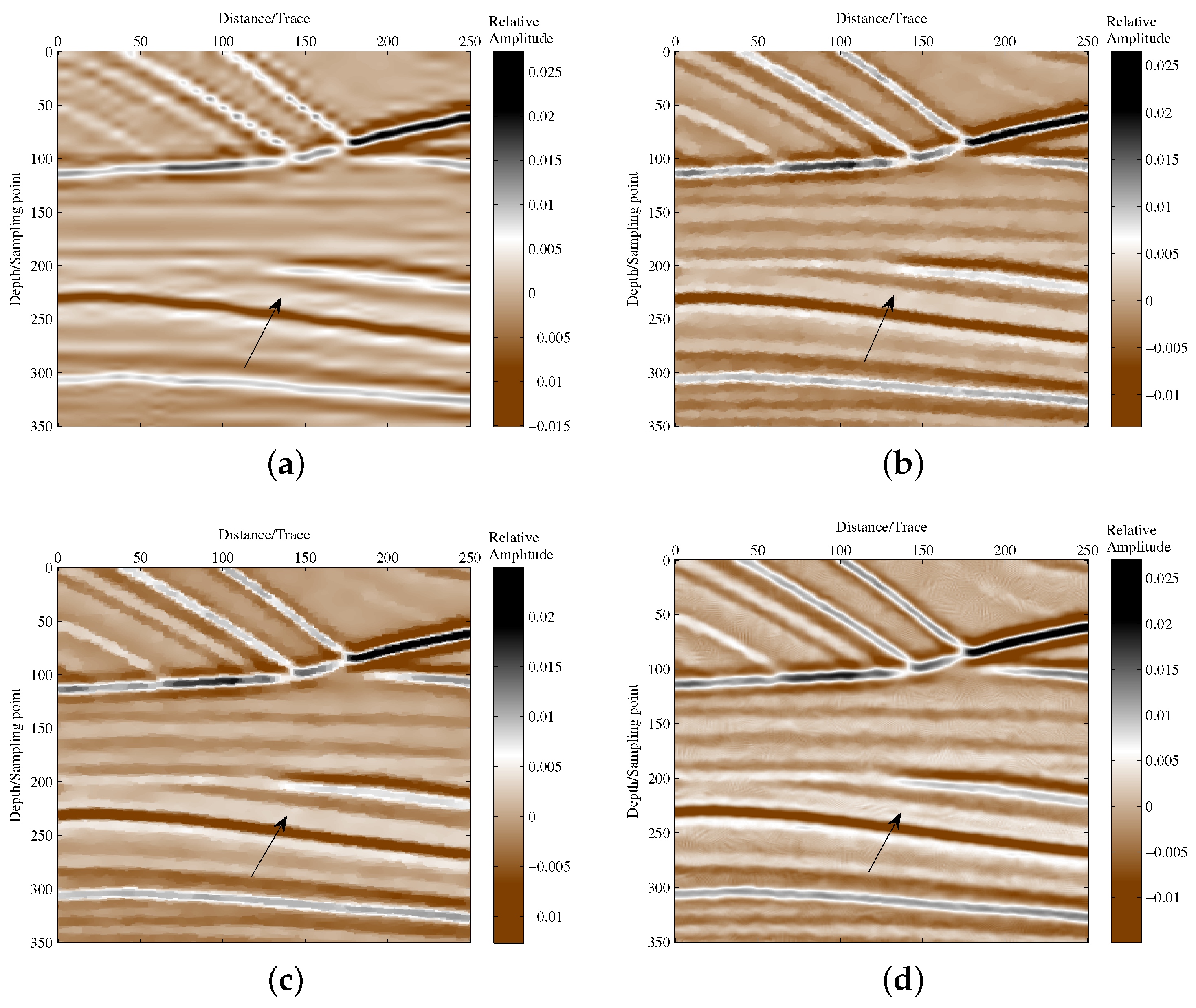
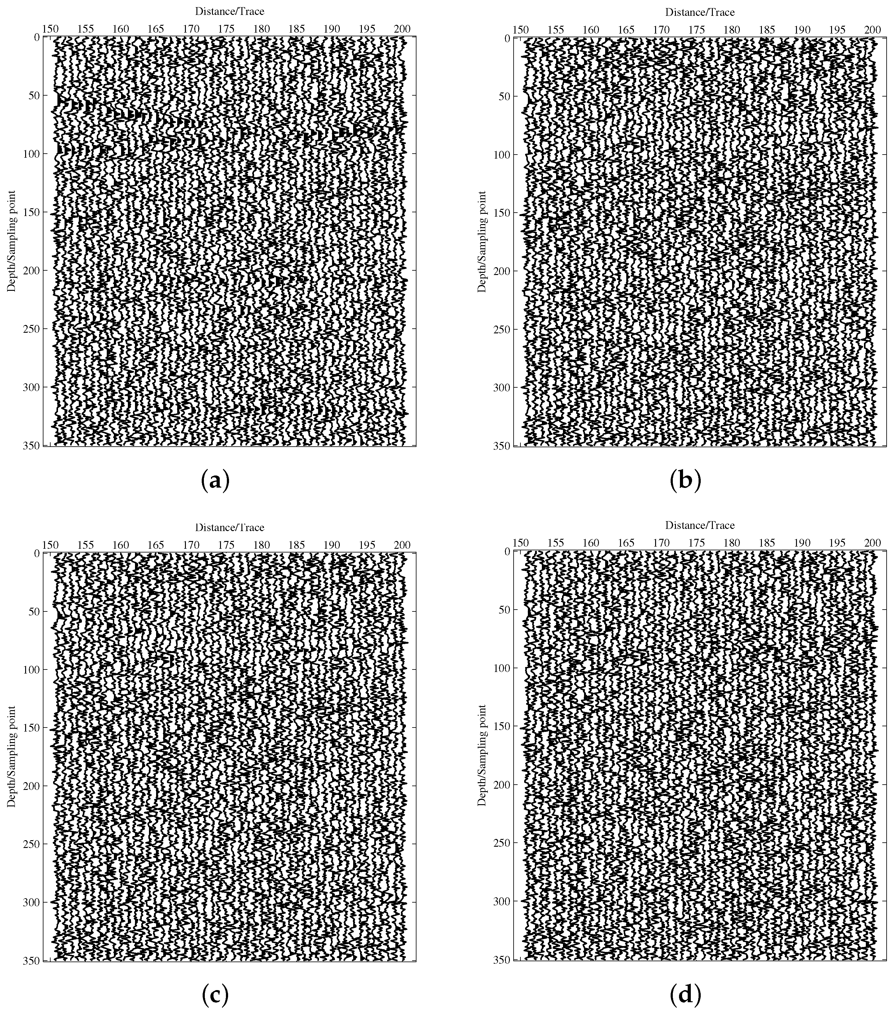
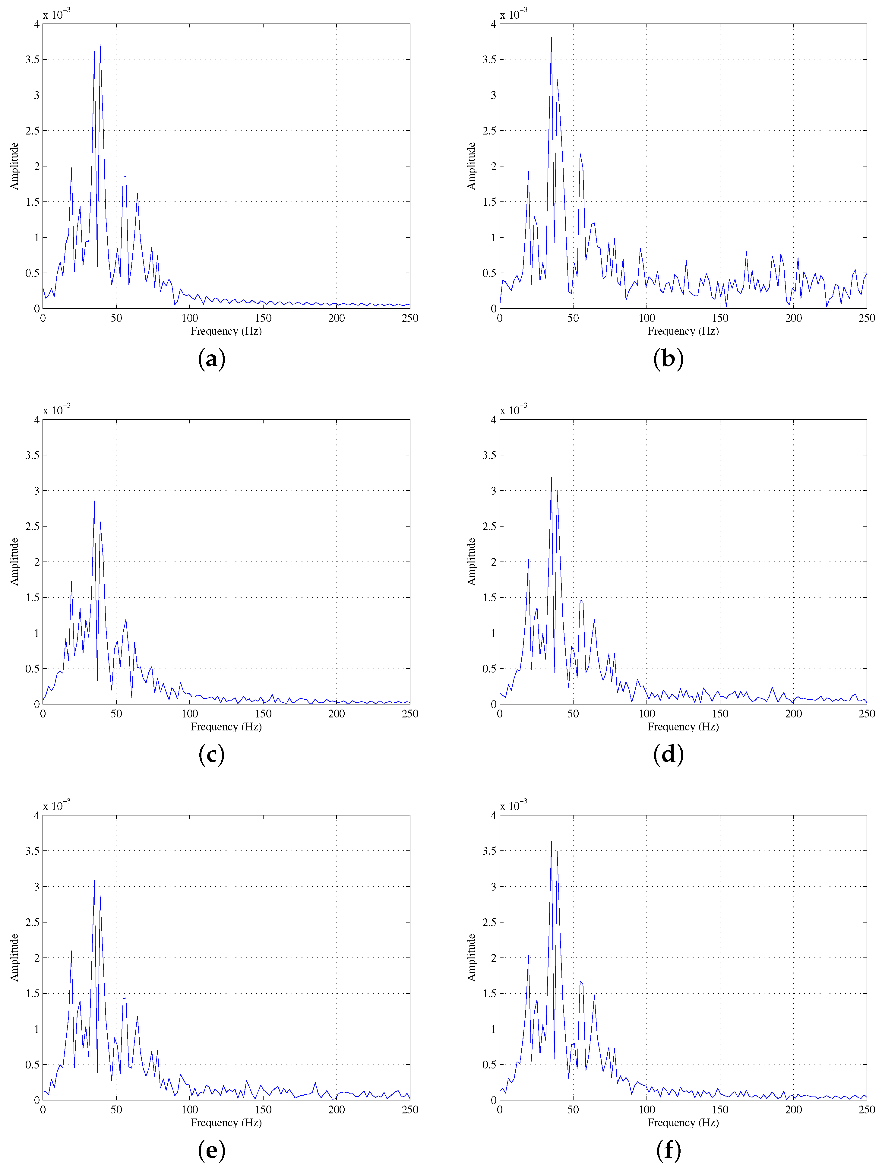
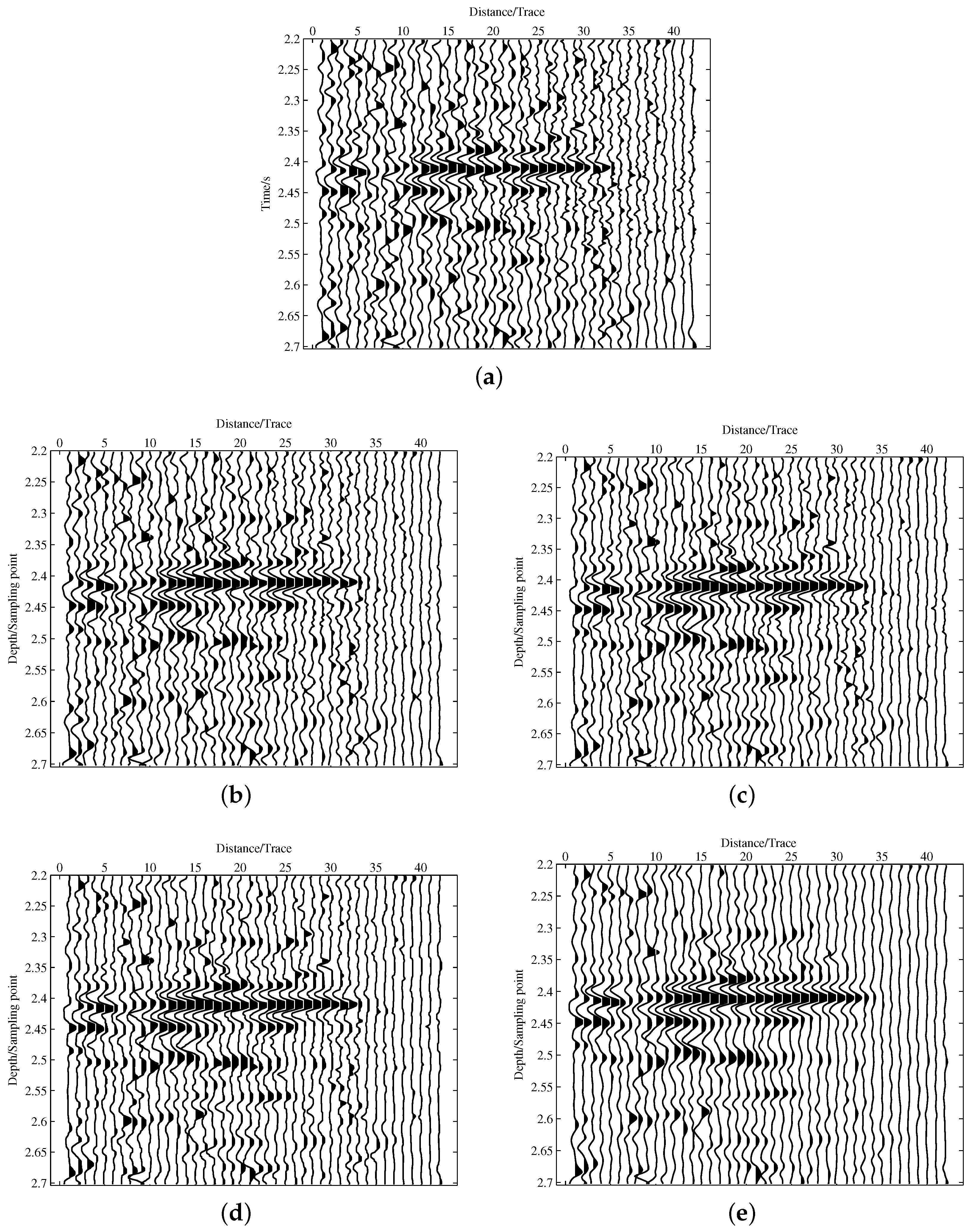
3. Numerical Experiments

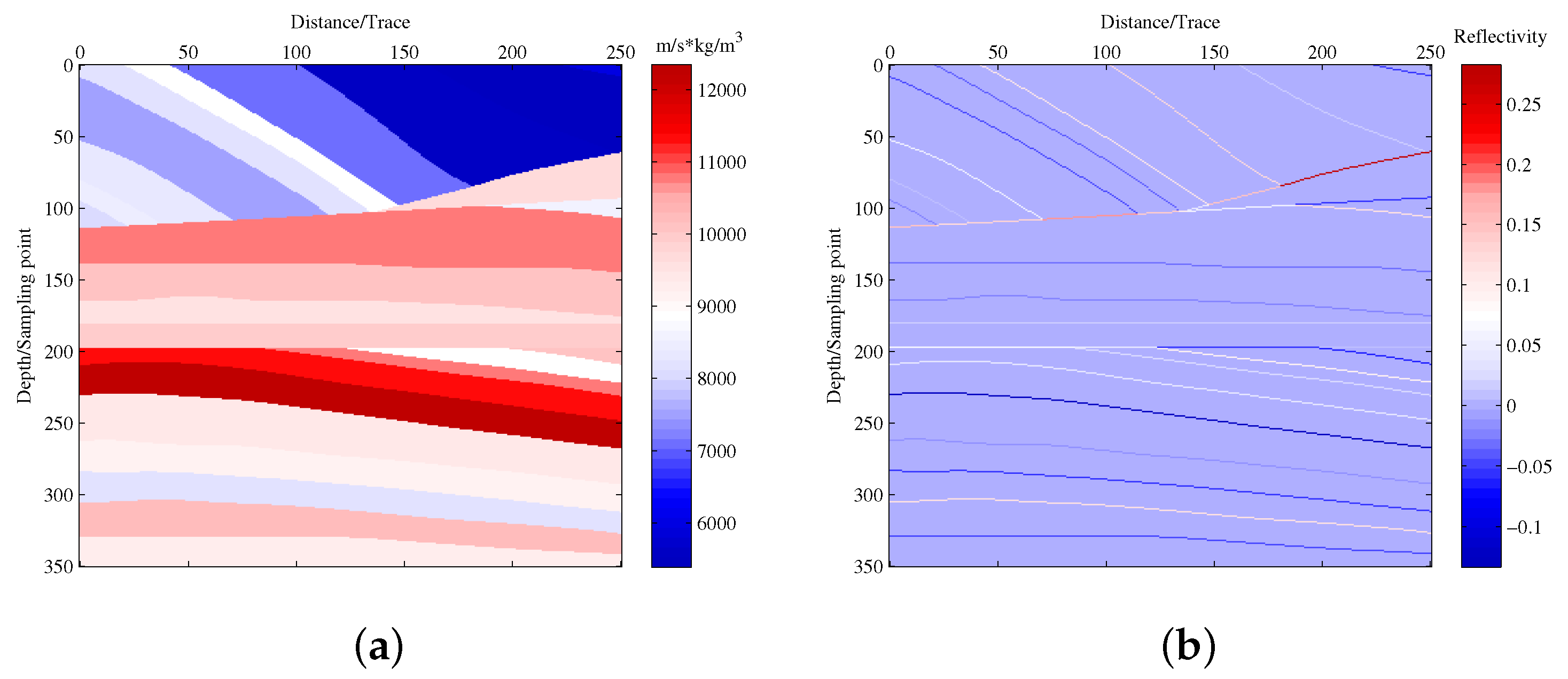
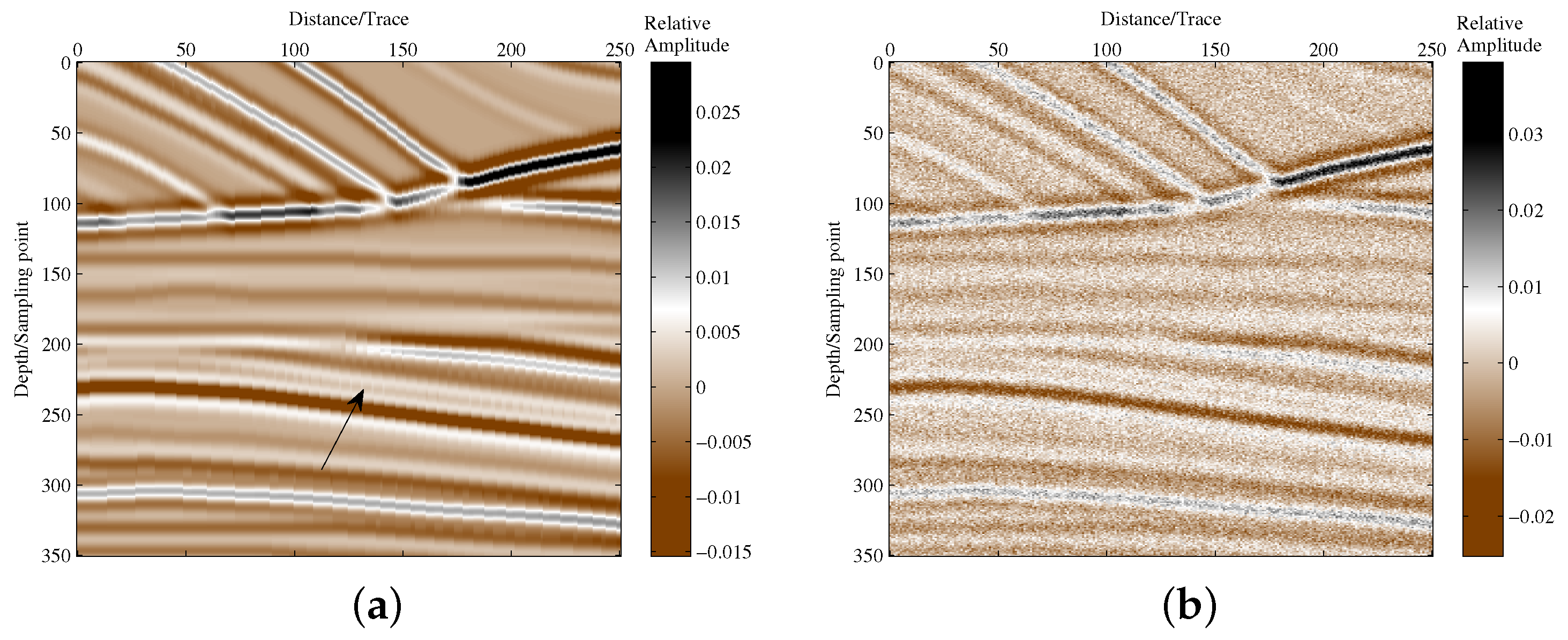
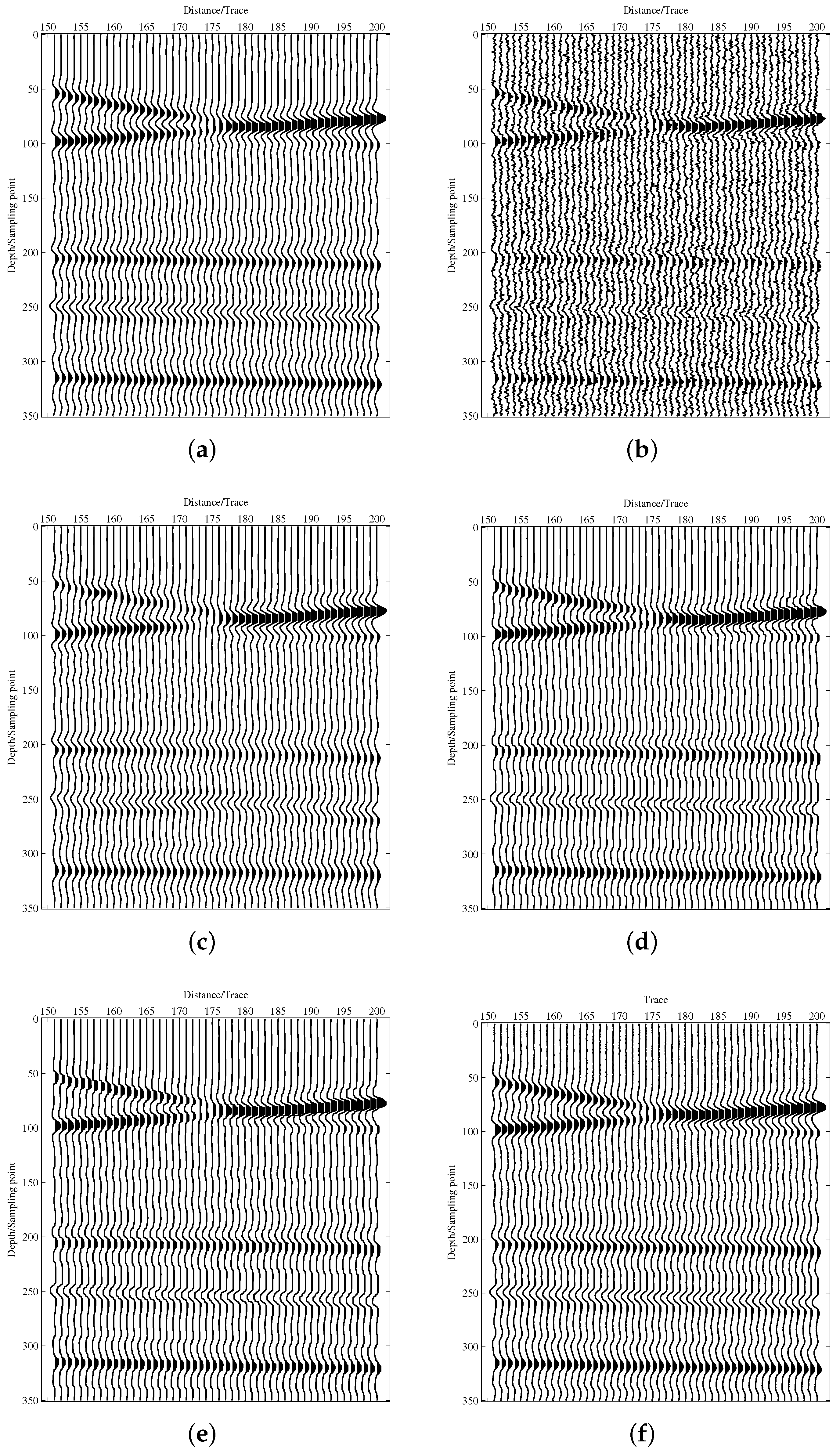
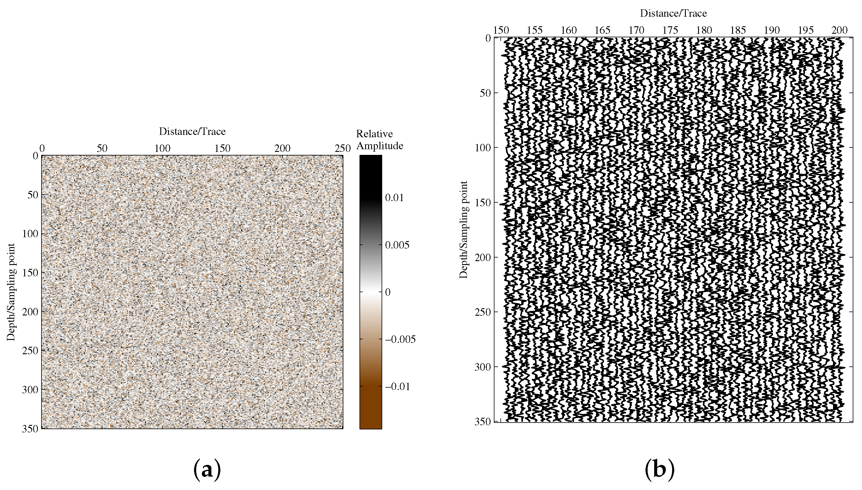
3.1. Synthetic Seismic Data Test

In this section, a synthetic seismic data test on the performance of the SD-SpaLR method is described. The data were obtained from the marmousi2 acoustic impedance (AI) model [24] by using the convolution operation. The AI model used is shown in Figure 1a, which consists of 251 seismic channels, each of which has 351 sampling points. The corresponding reflection coefficient section is shown in Figure 1b. It can be seen that the model is complex. Many strata with large dip angles and thin layers can be observed.

The synthetic seismic section without noise can be obtained by convoluting the reflection coefficient section shown in Figure 1b with a ricker wavelet whose dominant frequency is 40 Hz, as shown in Figure 2a. By adding Gaussian random noise to the noise-free seismic section, we can derive a noisy seismic section with signal-to-noise ratio (SNR) of 3 dB, which shown in Figure 2b. We can see that the noise in the noisy seismic section is very strong, and some weak reflection horizons have become blurred.

In order to compare the noise-free seismic section with the noisy section more clearly, waveforms of traces 151–200 in Figure 2a,b were extracted and displayed in Figure 3a,b respectively. Through careful observation and comparison of these two subgraphs, we can see that some of weak reflection waveforms in Figure 3a have been unrecognized in Figure 3b. For example, there is a weak flat layer above the 150th sampling point (see Figure 1b), which can be seen in Figure 3a but is submerged by noise in Figure 3b. Figure 4a,b shows the noise section added to the synthetic seismic data and the waveforms of the noise added to traces 151–200 respectively.

In this experiment, in addition to testing the performance of the SD-SpaLR method, three other methods are also compared. They are wavelet denoising, isotropic total variation denoising (ITVD) and anisotropic total variation denoising (ATVD). In the experiment of wavelet denoising, the wavelet decomposition function and denoising function were wavedec2 and wdencmp, respectively. They are built-in functions of MATLAB. The wavelet used was sym6 and the decomposition level was 5. ITVD and ATVD are based on the split Bregman iteration algorithm.

When the SNRs of input seismic data are 3 dB, 6 dB, 9 dB, 12 dB and 15 dB respectively, the regularization parameter of TV regularization terms in ITVD and ATVD are $4\times {10}^{-3}$, $2\times {10}^{-3}$, $1.5\times {10}^{-3}$, $1\times {10}^{-3}$ and $0.5\times {10}^{-3}$, respectively. The parameters of the SD-SpaLR method were set as: $\eta =\mu =1\times {10}^3$, $\alpha =2.5$ and $\beta =1.5$.

Figure 5 shows the denoising results of these four denoising methods for the synthetic seismic data with the SNR of 3 dB shown in Figure 2b. It can be seen that due to the strong noise, the wavelet denoising result deviates obviously from the true value, and many weak reflection layers can not be recovered. Both of the denoising results of ITVD method and ATVD method are better than that of the wavelet denoising method, but they cannot effectively protect the weak reflection signal. For instance, there is a weak reflection layer at the position indicated by the arrow (closely adjacent to the strong reflection layer below the arrow, which can be seen more clearly from Figure 2a), which cannot be observed from the denoising results of these two methods. Moreover, because these two methods are based on total variation, an obvious staircase effect can be observed in denoising results, which will damage the weak signal [25]. There is still a little noise in the denoising result of the SD-SpaLR method, but we can see that the SD-SpaLR method can effectively protect the weak signal, which is the only one of these four methods that can outline the weak reflection layer indicated by the arrow.

Figure 3c–f shows the waveforms of denoising results of traces 151–200 when the SNR of the seismic data is 3 dB. It can be seen that the waveforms of the denoising results are similar to the noise-free waveforms shown in Figure 3a. However, careful observation shows that useful signals in Figure 3c are weakened. The noise in Figure 3d,e is removed effectively, but many peaks and troughs are cut into trapezoids. This phenomenon is mainly due to the staircase effect caused by total variation. In Figure 3f, there are still some weak noise that has not been eliminated, but the denoising result is very close to the noise-free signal.

Figure 6 shows the waveforms of the filtered noise in traces 151 to 200 when the SNR of the input seismic data was 3 dB. It was obtained by subtracting the denoising results in Figure 3c–f from the noisy seismic data shown in Figure 3b. A comparison of Figure 6a with the noise-free signal shown in Figure 3a shows that the noise filtered by the wavelet denoising method contains obvious useful signals. If we observe carefully, it is not difficult to find that the noise filtered by ITVD and ATVD, which is shown in Figure 6b,c also contains weak useful signals. The damage to useful signals is more obvious in the position of two intersecting events between the 50th and 100th sampling points. Figure 6d shows that the SD-SpaLR method does not remove useful signals obviously.

In order to quantitatively compare the denoising performances of these four methods, we calculated the SNRs of the denoising results when the SNR of the input noisy seismic data was 3 dB, 6 dB, 9 dB, 12 dB and 15 dB respectively, and we have shown them in

Table 1. Variation of the SNR of denoising results with the SNR of the input seismic data.

SNR of the input seismic data (dB)	3	6	9	12	15
SNR of wavelet denoising (dB)	8.39	10.92	12.97	14.95	16.89
SNR of ITVD (dB)	12.64	14.91	16.77	18.76	20.61
SNR of ATVD (dB)	11.90	14.74	15.51	18.59	20.97
SNR of SD-SpaLR (dB)	16.34	18.18	19.52	20.40	21.03

. It can be seen that the SNR of wavelet denoising is the lowest, and the SD-SpaLR method has the highest SNR. The denoising performances of ITVD and ATVD were close. It can also be found that the lower the SNR of the input seismic data is, the higher the SNR of the SD-SpaLR method is compared to those SNRs of three other methods. In this experiment, the formula for calculating the SNR was:

$$SNR=10lg\frac{{∥\mathbf{S}∥}_F^2}{{∥\mathbf{S}-{\mathbf{S}}_d∥}_F^2},$$

(19)

where $\mathbf{S}$ and ${\mathbf{S}}_d$ denote noise-free seismic data and denoised seismic data respectively.

In denoising applications there is an index called structural similarity (SSIM) [26], which can be used to evaluate the structural similarity between the denoised result and the noise-free data. The maximum value of SSIM is 1. The larger the SSIM value is, the more similar the structure between the denoising result and the noise-free data is. The SSIM between two images $\mathbf{X}$ and $\mathbf{Y}$ is calculated by [26]

$$SSIM(\mathbf{X},\mathbf{Y})=\frac{\left(2{\mu }_X{\mu }_Y+C_1\right)\left(2{\sigma }_{XY}+C_2\right)}{\left({\mu }_X^2+{\mu }_Y^2+C_1\right)\left({\sigma }_X^2+{\sigma }_Y^2+C_2\right)},$$

(20)

where ${\mu }_X$ and ${\mu }_Y$ are the mean of $\mathbf{X}$ and $\mathbf{Y}$ respectively. ${\sigma }_X^2$ and ${\sigma }_Y^2$ denote the variance of $\mathbf{X}$ and $\mathbf{Y}$ respectively. The values of $C_1={\left(Z{K}_1\right)}^2$ and $C_2={\left(Z{K}_2\right)}^2$ are usually very small and are mainly used to prevent the denominator from approaching 0. Here, $Z=200$, and $K_1=K_2=5\times {10}^{-6}$. The formula for calculating ${\sigma }_{XY}$ is given by

$${\sigma }_{XY}=\frac{1}{N-1}\sum _{i=1}^N\left(X_i-{\mu }_X\right)\left(Y_i-{\mu }_Y\right),$$

(21)

where N stands for the number of elements in $\mathbf{X}$ or $\mathbf{Y}$.

Table 2. Variation of structural similarity (SSIM) with the SNR of the input seismic data.

SNR of the input data (dB)	3	6	9	12	15
SSIM of wavelet denoising	0.68	0.77	0.84	0.9	0.93
SSIM of ITVD	0.83	0.89	0.93	0.95	0.97
SSIM of ATVD	0.81	0.89	0.93	0.95	0.97
SSIM of SD-SpaLR	0.90	0.94	0.96	0.98	0.98

shows the SSIM values between the denoising results and the noise-free seismic data when the SNRs of the input noisy data were 3 dB, 6 dB, 9 dB, 12 dB and 15 dB respectively. It is not difficult to find that the SSIM value increases with the increase of the SNR of the input noisy data. The SSIM value of wavelet denoising was the lowest. The SSIM values of ITVD and ATVD were very close. The SD-SpaLR method had the largest SSIM value. This shows that the denoising result of the SD-SpaLR method is most similar to the original noise-free seismic data.

In order to observe and compare denoising results in the frequency domain, Figure 7 shows the amplitude spectrum of trace 100 of noise-free data, that of the noisy data when the SNR is 3 dB and that of the denoising results by four methods mentioned above. For ease of observation, only frequency components no higher than 250 Hz are plotted. We can see that wavelet denoising has the best effect on the suppression of noise of frequency higher than 100 Hz. However, its damage to useful signals whose frequency lower than 100 Hz is also the most serious. In the denoising results of ITVD and ATVD we can observe apparent noise when the frequency is higher than 100 Hz, and whose noise amplitudes are higher than those of wavelet denoising and the SD-SpaLR methods in this frequency band. The amplitude spectrum of the denoising result of the SD-SpaLR method is consistent with that of the noise-free data, and the noise of frequency higher than 100 Hz is also very weak.

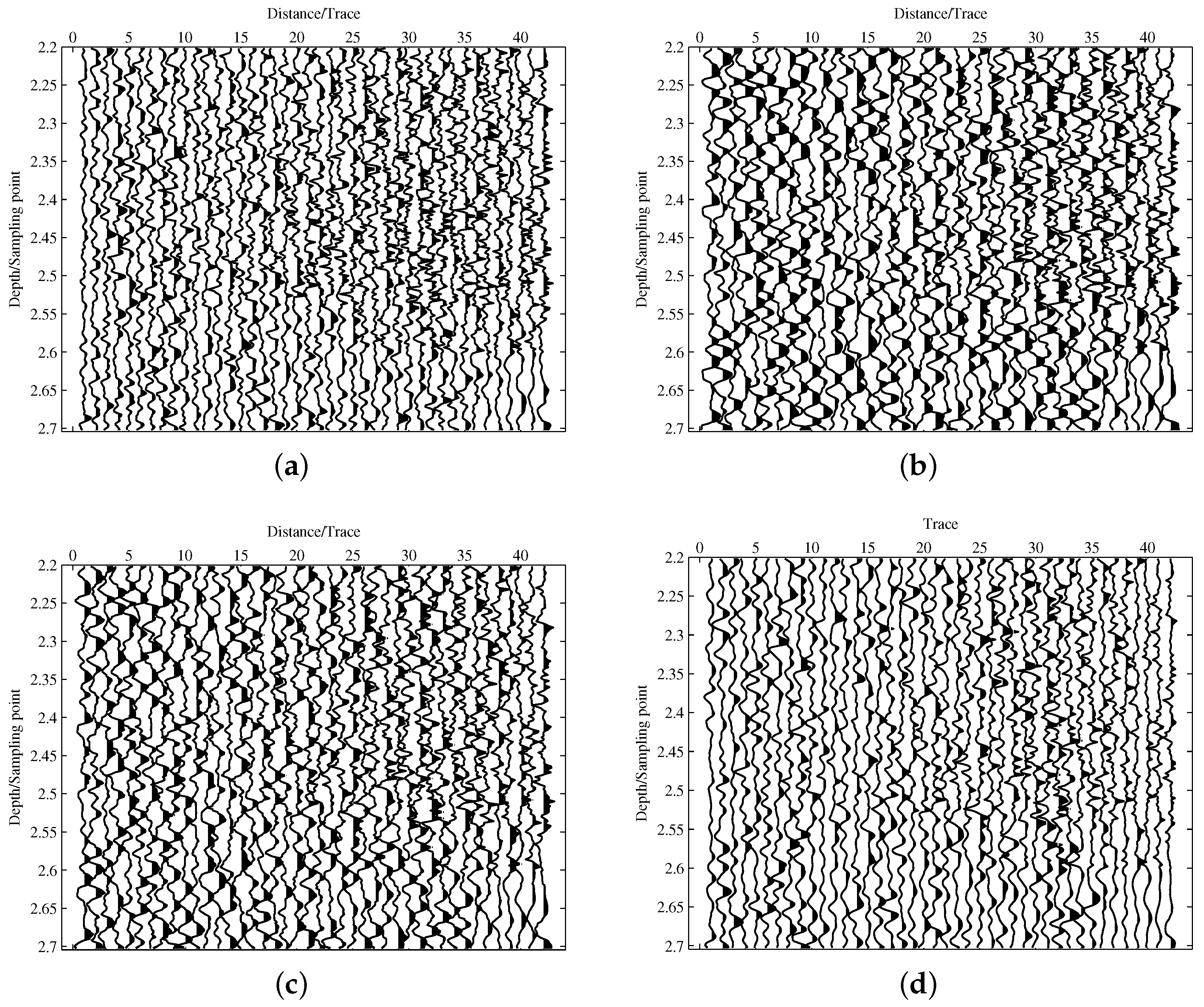
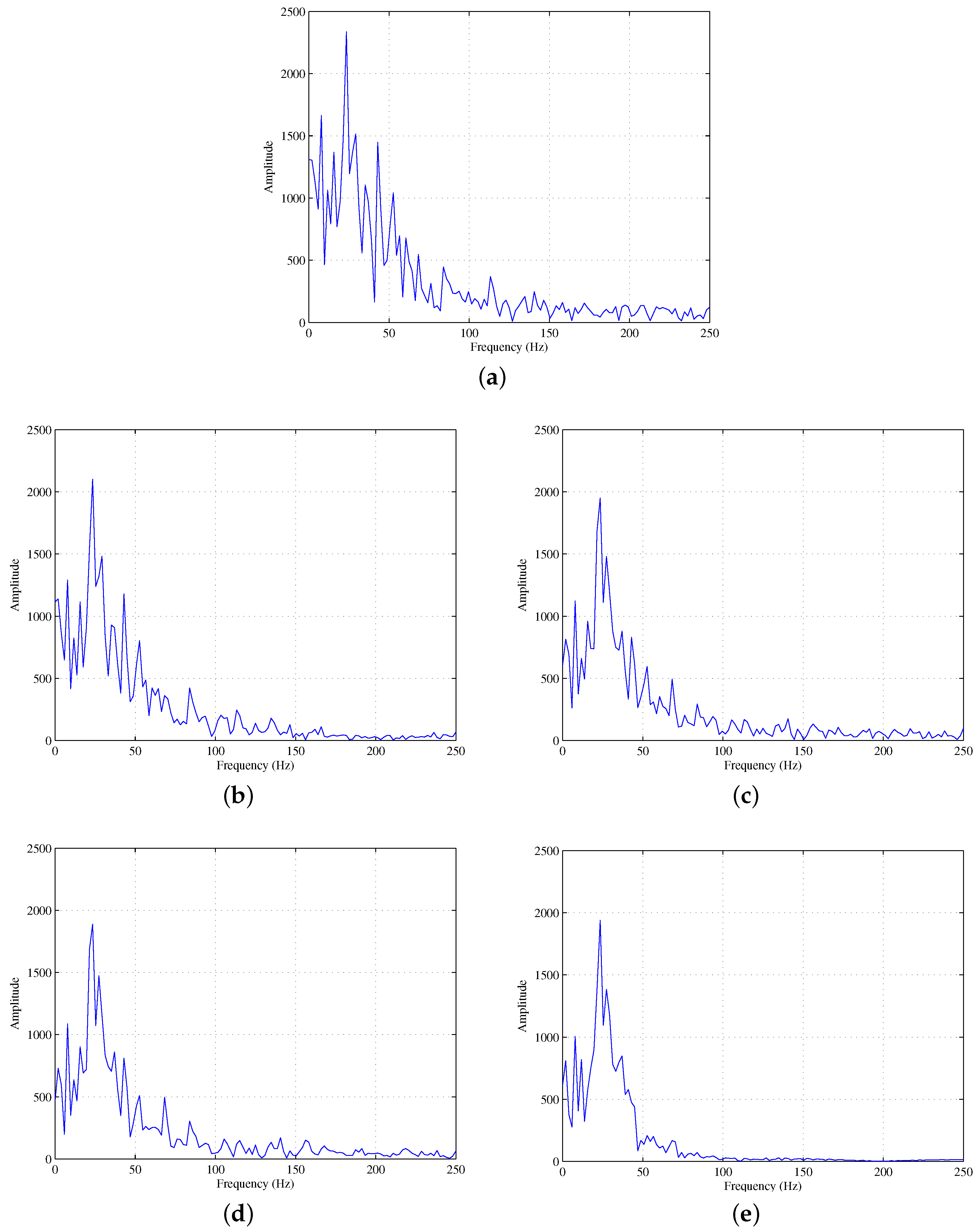
3.2. Field Seismic Data Test

In this experiment, field-gathered seismic data were used to test and compare the denoising performances of the methods mentioned above. Figure 8a shows the data, which are a part of a prestack angle gathered and acquired from an oil field in China. They consist of 42 seismic traces. There are 251 sampling points in each trace and the sampling interval is 2 ms. It can be seen that the data are contaminated by noise. In the area where the trace number is greater than 20 and the time is less than 2.55 s (the upper right part in Figure 8a), the high-frequency noise is particularly obvious. This phenomenon is due to the low amplitude of the useful signals acquired in the large angle area. Therefore, the impact of noise on the data in this area is more obvious.

Figure 8b–e show the denoising results of wavelet denoising, ITVD, ATVD and SD-SpaLR. Compared with the field seismic data, we can see that the noise in these figures is attenuated. Through careful observation, we can find that the denoising result of the SD-SpaLR method is the best, and the seismic events in Figure 8e are very clear. Especially in the region with high-frequency noise (the upper right part of Figure 8a), the SD-SpaLR method suppresses the noise most successfully.

In order to evaluate the effect of denoising methods on noise attenuation, we calculated the difference between the original field seismic data shown in Figure 8a and the denoising results shown in Figure 8b–e respectively. Those differences can be regarded as the noise removed by different denoising methods. They are shown in Figure 9a–d respectively.

We can see that these methods can effectively suppress the high-frequency noise in the upper right part of Figure 8a. In addition, it can also be found from Figure 9b,c that in the area with high-frequency noise (upper right corner part), the amplitude of the noise removed is relatively small, while in other areas the amplitude of the noise removed is relatively large. This means that ITVD and ATVD may also have removed useful signals. On the contrary, the wavelet denoising and SD-SpaLR methods had little influence on useful signals.

Figure 10 shows the amplitude spectrum of denoising results of trace 30. From Figure 10a, we can see that the dominant frequency of useful signals is about 23 Hz, and there is a lot of noise when the frequency is higher than 100 Hz. Figure 10b–e shows the amplitude spectrum of denoising results by wavelet denoising, ITVD, ATVD and SD-SpaLR respectively. It can be seen that all these four methods can attenuate the high-frequency noise with frequency higher than 100 Hz. However, only SD-SpaLR can almost perfectly suppress the noise in this frequency band.

4. Conclusions

By using a data-driven sparse transformation learning method and low-rank constraint based on block matching, we presented a seismic data denoising method which combines the local sparsity with the nonlocal self-similarity of seismic data. The proposed method was tested with 2-D synthetic seismic data and a part of the field data from a prestack angle gather. The denoising results of this method were compared with those of wavelet denoising, isotropic total variation denoising and anisotropic total variation denoising. The experimental results showed that the proposed method could get the highest SNR and SSIM. In addition, the experimental results also showed that the method proposed in this paper could not only suppress noise most effectively, but also had little influence on useful signals. The proposed method had better denoising performance than other methods, mainly due to the joint use of the sparsity and self-similarity of the seismic data.

In the field of seismic reconstruction, scholars also used sparse regularization or low-rank regularization, but they did not combine these two regularization methods. The research on the seismic data reconstruction method combining sparse and low-rank regularization will be our future work.

References

1. Jiang, T.; Lin, J.; Li, T.L.; Chen, Z.B.; Zhang, L.H. Boosting Signal to Noise Ratio of Seismic Signals Using the Phased-Array Vibrator System. Chin. J. Geophys. 2006, 49, 1658–1664. [Google Scholar] [CrossRef]
2. Canales, L.L. Random noise reduction. In SEG Technical Program Expanded Abstracts 1984; Society of Exploration Geophysicists: Tulsa, OK, USA, 1984; pp. 525–527. [Google Scholar]
3. Wang, Y. Inverse Q-filter for seismic resolution enhancement. Geophysics 2006, 71, V51–V60. [Google Scholar] [CrossRef] [Green Version]
4. Cao, S.; Chen, X. The second-generation wavelet transform and its application in denoising of seismic data. Appl. Geophys. 2005, 2, 70–74. [Google Scholar] [CrossRef]
5. Zhai, M.Y. Seismic data denoising based on the fractional Fourier transformation. J. Appl. Geophys. 2014, 109, 62–70. [Google Scholar] [CrossRef]
6. Neelamani, R.; Baumstein, A.I.; Gillard, D.G.; Hadidi, M.T.; Soroka, W.L. Coherent and random noise attenuation using the curvelet transform. Lead. Edge 2008, 27, 240–248. [Google Scholar] [CrossRef]
7. Kong, D.; Peng, Z. Seismic random noise attenuation using shearlet and total generalized variation. J. Geophys. Eng. 2015, 12, 1024–1035. [Google Scholar] [CrossRef] [Green Version]
8. Tang, G.; Ma, J. Application of total-variation-based curvelet shrinkage for three-dimensional seismic data denoising. IEEE Geosci. Remote Sens. Lett. 2011, 8, 103–107. [Google Scholar] [CrossRef]
9. Chen, Y.; Peng, Z.; Li, M.; Yu, F. Random noise suppression based on the improved total generalized variation with overlapping group sparsity. Oil Geophys. Prospect. 2019, 54, 24–35. (In Chinese) [Google Scholar]
10. Bonar, D.; Sacchi, M. Denoising seismic data using the nonlocal means algorithm. Geophysics 2012, 77, A5–A8. [Google Scholar] [CrossRef]
11. Chen, Y.; Ma, J.; Fomel, S. Double-sparsity dictionary for seismic noise attenuation. Geophysics 2016, 81, V103–V116. [Google Scholar] [CrossRef]
12. Ghaderpour, E.; Liao, W.; Lamoureux, M.P. Antileakage least-squares spectral analysis for seismic data regularization and random noise attenuation. Geophysics 2018, 83, V157–V170. [Google Scholar] [CrossRef]
13. Ghaderpour, E. Multichannel antileakage least-squares spectral analysis for seismic data regularization beyond aliasing. Acta Geophys. 2019, 67, 1349–1363. [Google Scholar] [CrossRef]
14. Wen, B.; Li, Y.; Bresler, Y. When sparsity meets low-rankness: Transform learning with non-local low-rank constraint for image restoration. In Proceedings of the IEEE International Conference on Acoustics, Speech and Signal Processing, New Orleans, LA, USA, 5–9 March 2017; pp. 2297–2301. [Google Scholar]
15. Dabov, K.; Foi, A.; Katkovnik, V.; Egiazarian, K. Image denoising by sparse 3-D transform-domain collaborative filtering. IEEE Trans. Image Process. 2007, 16, 2080–2095. [Google Scholar] [CrossRef]
16. Tang, G.; Ma, J.W.; Yang, H.Z. Seismic data denoising based on learning-type overcomplete dictionaries. Appl. Geophys. 2012, 9, 27–32. [Google Scholar] [CrossRef]
17. Fomel, S.; Liu, Y. Seislet transform and seislet frame. Geophysics 2010, 75, V25–V38. [Google Scholar] [CrossRef] [Green Version]
18. Yu, G.; Sapiro, G. DCT image denoising: A simple and effective image denoising algorithm. Image Process. Line 2011, 1, 292–296. [Google Scholar] [CrossRef] [Green Version]
19. Kumar, P.; Foufoula-Georgiou, E. Wavelet analysis for geophysical applications. Rev. Geophys. 1997, 35, 385–412. [Google Scholar] [CrossRef] [Green Version]
20. Zhou, Y.; Li, S.; Xie, J.; Zhang, D.; Chen, Y. Sparse dictionary learning for seismic noise attenuation using a fast orthogonal matching pursuit algorithm. J. Seism. Explor. 2017, 26, 433–454. [Google Scholar]
21. Elad, M.; Aharon, M. Image denoising via sparse and redundant representations over learned dictionaries. IEEE Trans. Image Process. 2006, 15, 3736–3745. [Google Scholar] [CrossRef]
22. Ravishankar, S.; Bresler, Y. l0 sparsifying transform learning with efficient optimal updates and convergence guarantees. IEEE Trans. Signal Process. 2015, 63, 2389–2404. [Google Scholar] [CrossRef]
23. Wen, B.; Li, Y.; Bresler, Y. The power of complementary regularizers: Image recovery via transform learning and low-rank modeling. arXiv 2018, arXiv:1808.01316. [Google Scholar]
24. Martin, G.S.; Wiley, R.; Marfurt, K.J. Marmousi2: An elastic upgrade for Marmousi. Lead. Edge 2006, 25, 156–166. [Google Scholar] [CrossRef]
25. Bredies, K.; Kunisch, K.; Pock, T. Total generalized variation. SIAM J. Imaging Sci. 2010, 3, 492–526. [Google Scholar] [CrossRef]
26. Wang, Z.; Bovik, A.C.; Sheikh, H.R.; Simoncelli, E.P. Image quality assessment: From error visibility to structural similarity. IEEE Trans. Image Process. 2004, 13, 600–612. [Google Scholar] [CrossRef] [Green Version]
Figure 1. Acoustic impedance section and its reflection coefficient section for generating synthetic seismic data. (a) Acoustic impedance section; (b) reflection coefficient section.
Energies 13 00372 g001
Figure 2. (a) A noise-free seismic section and (b) a noisy seismic section with a signal-to-noise ratio (SNR) of 3 dB.
Energies 13 00372 g002
Figure 3. Waveforms of the denoising result of traces 151–200 from Figure 2 while the SNR of the input seismic data was 3 dB. (a) Noise-free waveforms, (b) noisy waveforms with the SNR of 3 dB, (c) wavelet denoising result, (d) isotropic total variation denoising (ITVD) result, (e) anisotropic total variation denoising (ATVD) result and (f) SD-SpaLR result.
Energies 13 00372 g003
Figure 4. (a) Noise section; (b) Waveforms of noise added to traces 151 to 200.
Energies 13 00372 g004
Figure 5. Denoising results of noisy seismic data with the SNR of 3 dB. (a) Wavelet denoising result, (b) ITVD result, (c) ATVD result and (d) SD-SpaLR result.
Energies 13 00372 g005
Figure 6. Waveforms of the filtered noise in traces 151–200 when the SNR of the input seismic data was 3 dB. (a) Filtered noise by wavelet denoising, (b) filtered noise by ITVD, (c) filtered noise by ATVD and (d) filtered noise by the SD-SpaLR method.
Energies 13 00372 g006
Figure 7. Amplitude spectrum of the denoising result of trace 100 when the SNR of the input noisy seismic signal was 3 dB. (a) Spectrum of the noise-free data, (b) spectrum of the input noisy data, (c) spectrum of the wavelet denoising result, (d) spectrum of the ITVD result, (e) spectrum of the ATVD result and (f) spectrum of the SD-SpaLR method.
Energies 13 00372 g007
Figure 8. Field seismic data and its denoising results. (a) Field seismic data, (b) wavelet denoising result, (c) ITVD result, (d) ATVD result and (e) denoising result of the SD-SpaLR method.
Energies 13 00372 g008
Figure 9. Noise removed by different denoising methods. (a) Noise removed by wavelet denoising, (b) noise removed by ITVD, (c) noise removed by ATVD and (d) noise removed by the SD-SpaLR method.
Energies 13 00372 g009
Figure 10. Amplitude spectrum of denoising results of trace 30. (a) Amplitude spectrum of the noise-free seiemic data, (b) amplitude spectrum of the wavelet denoising result, (c) amplitude spectrum of the ITVD result, (d) amplitude spectrum of the ATVD result and (e) amplitude spectrum of the denoising result by the SD-SpaLR method.
Energies 13 00372 g010