Back Analysis of the Initial Geo-Stress Field of Rock Masses in High Geo-Temperature and High Geo-Stress

Abstract
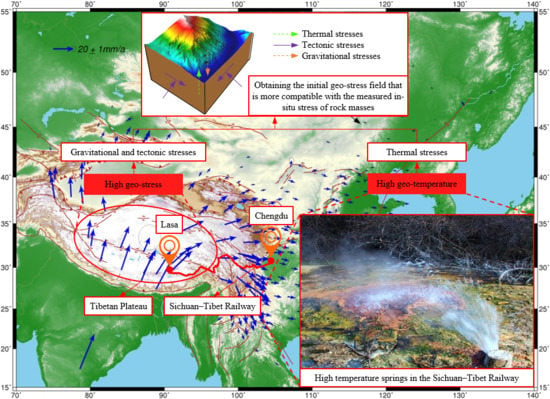
1. Introduction
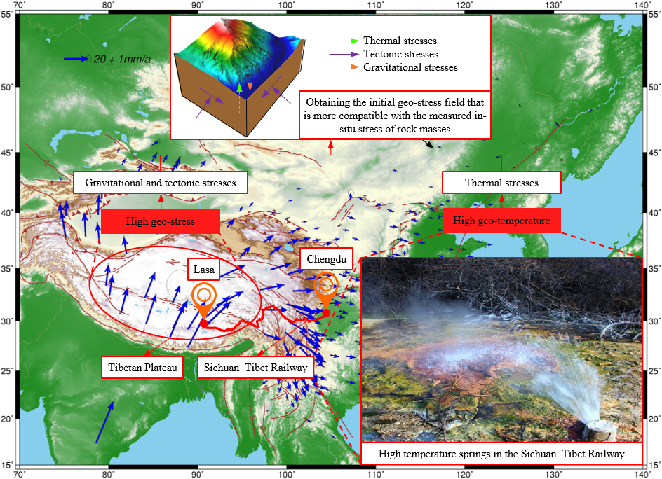
2. The Thermal Stress of Rock Masses Caused by Geothermal Gradients
3. The Measurement Principles of the Hydraulic Fracturing and Overcoring Methods
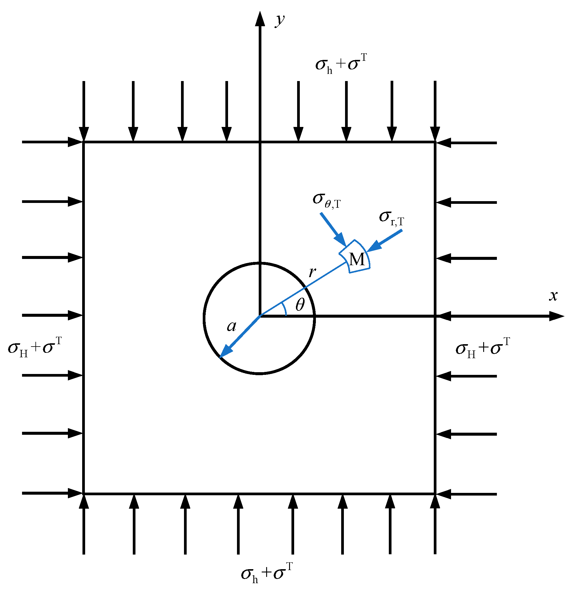
3.1. The Measurement Principle of the Hydraulic Fracturing Method in a Non-High Geo-Temperature Environment
3.2. The Measurement Principle of the Hydraulic Fracturing Method in a High Geo-Temperature Environment
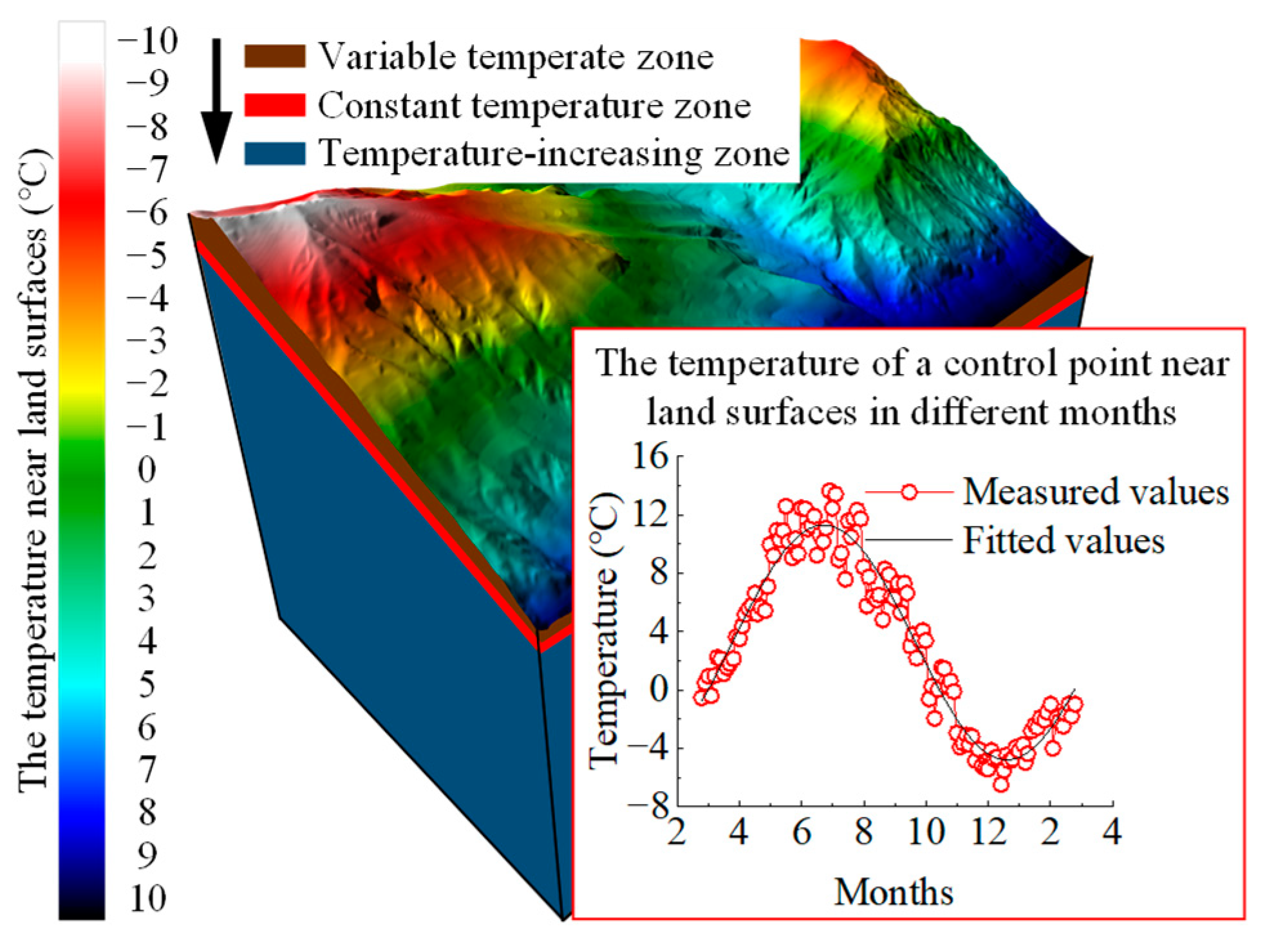
3.3. The Measurement Principle of Overcoring Methods
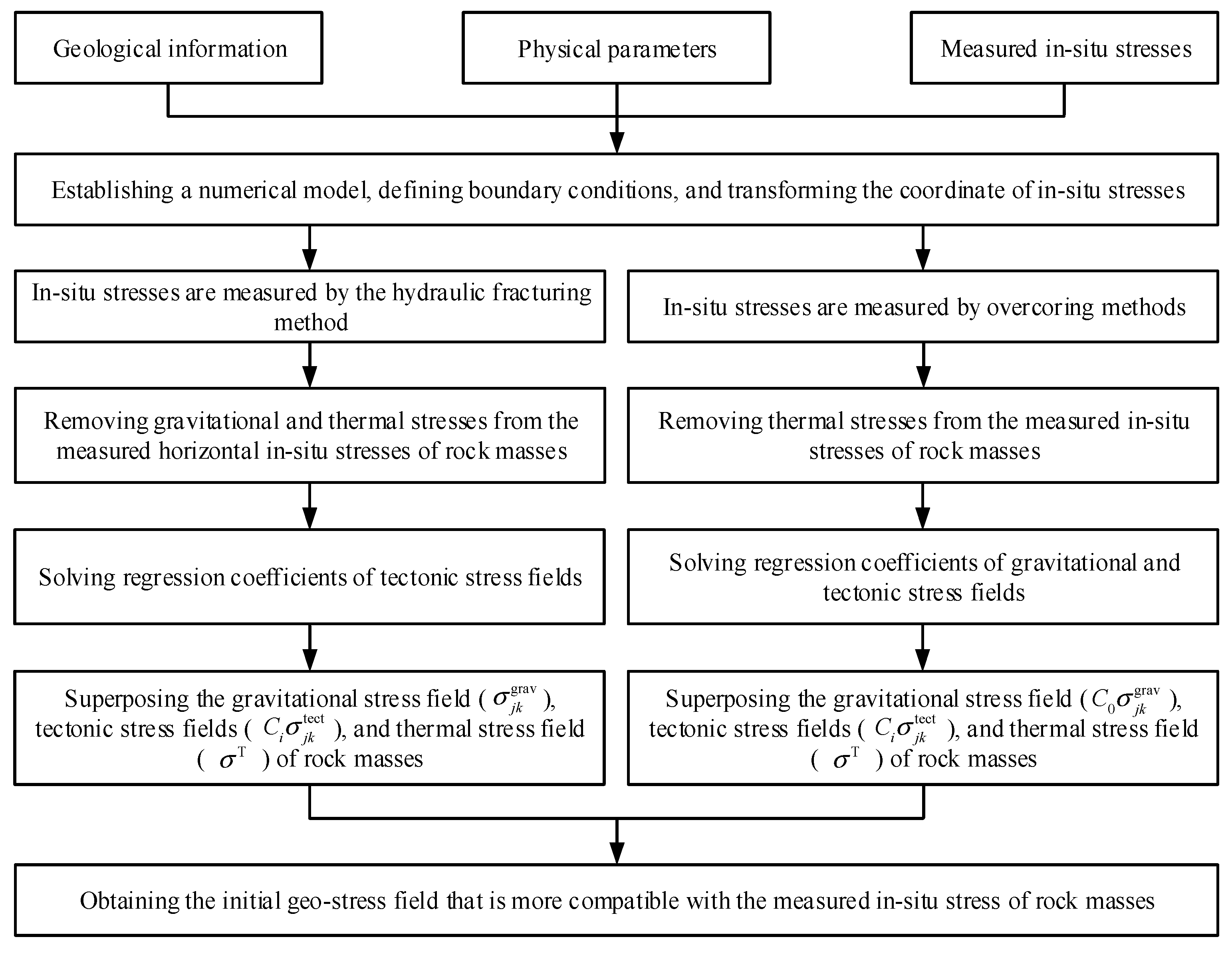
4. The Workflow for a Back Analysis Considering Geo-Temperature
4.1. In Situ Stresses Are Measured by the Hydraulic Fracturing Method
4.2. In Situ Stresses Are Measured by Overcoring Methods
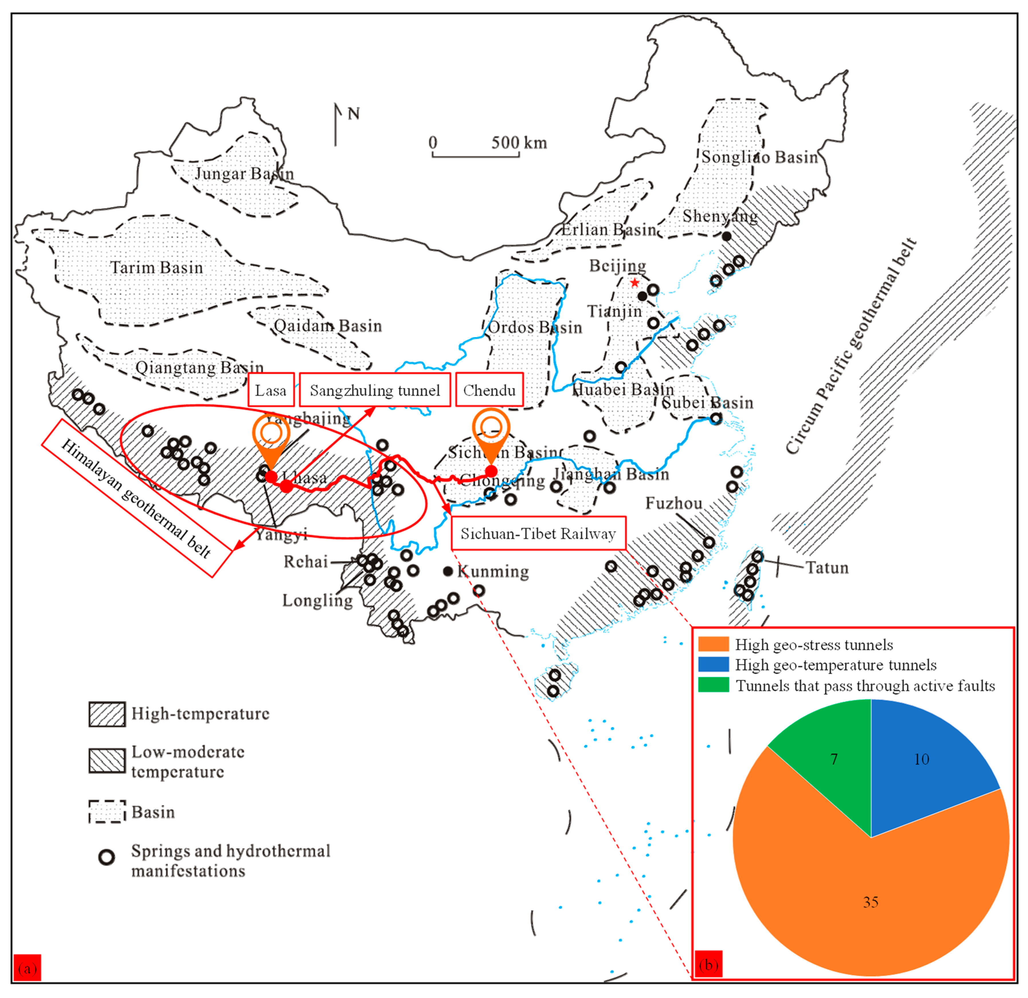
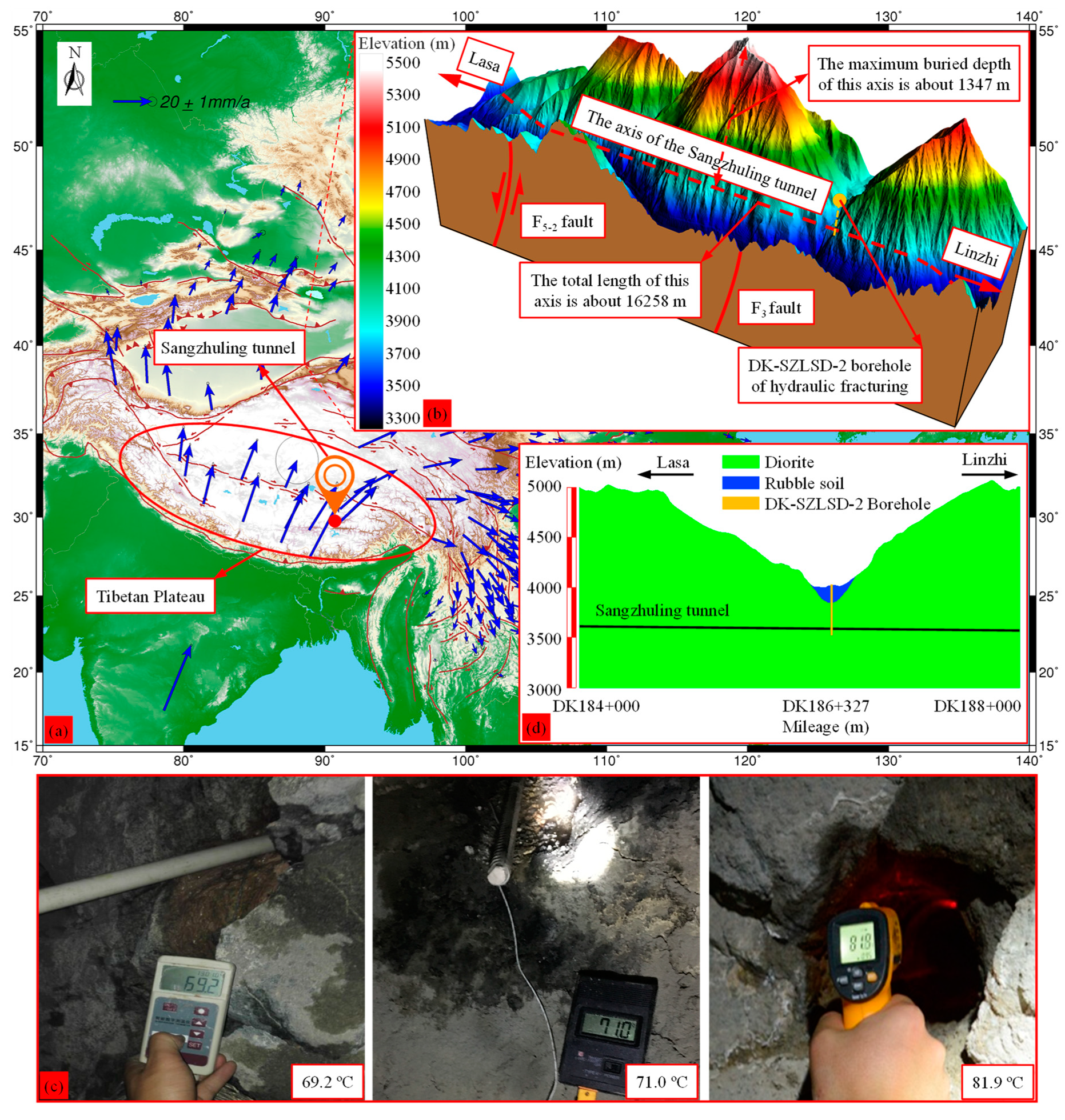
5. Engineering Application: A Case Study
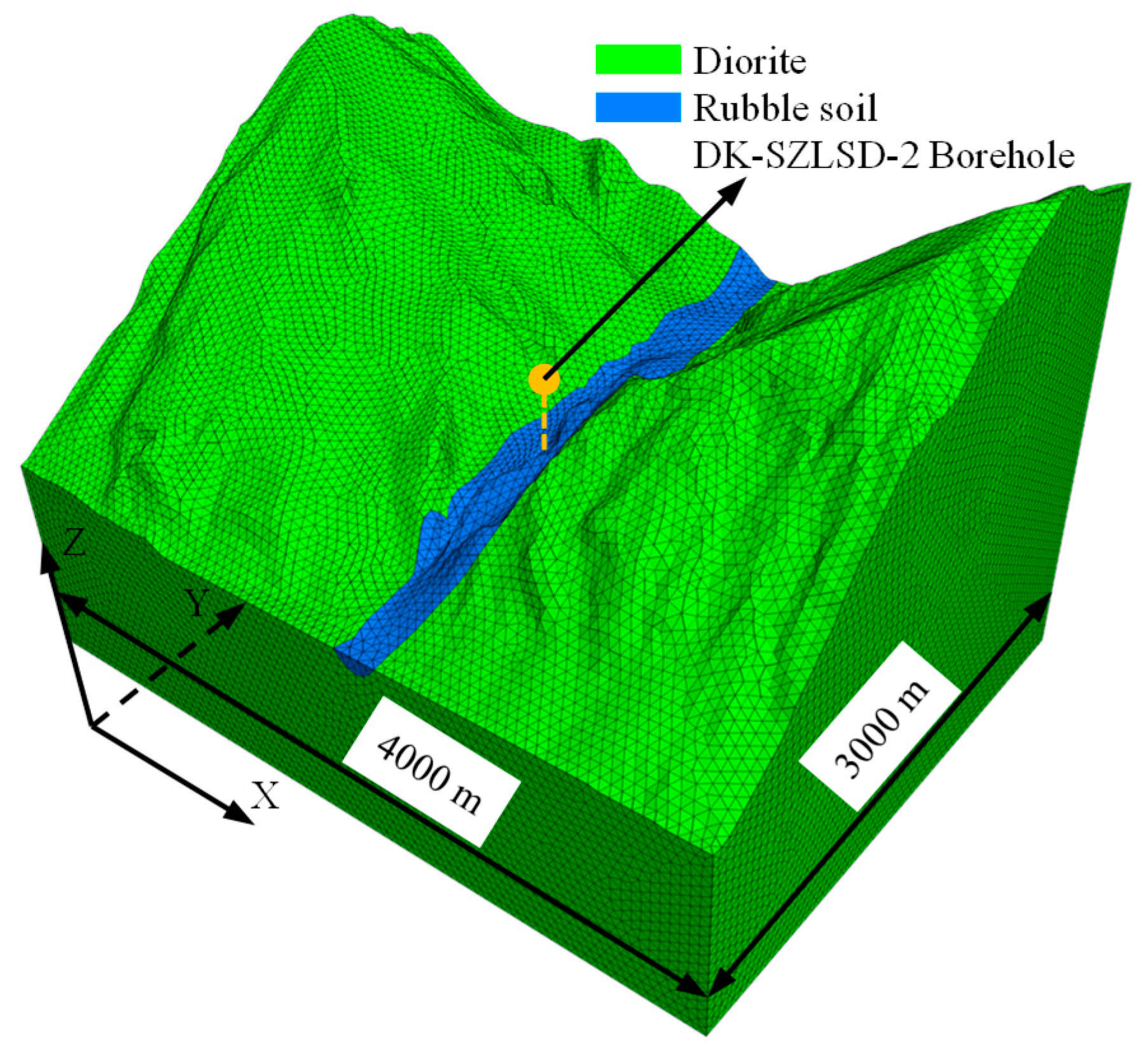
5.1. Project Overview
5.2. Establishing a Three-Dimensional Numerical Model
5.3. Defining Boundary Conditions
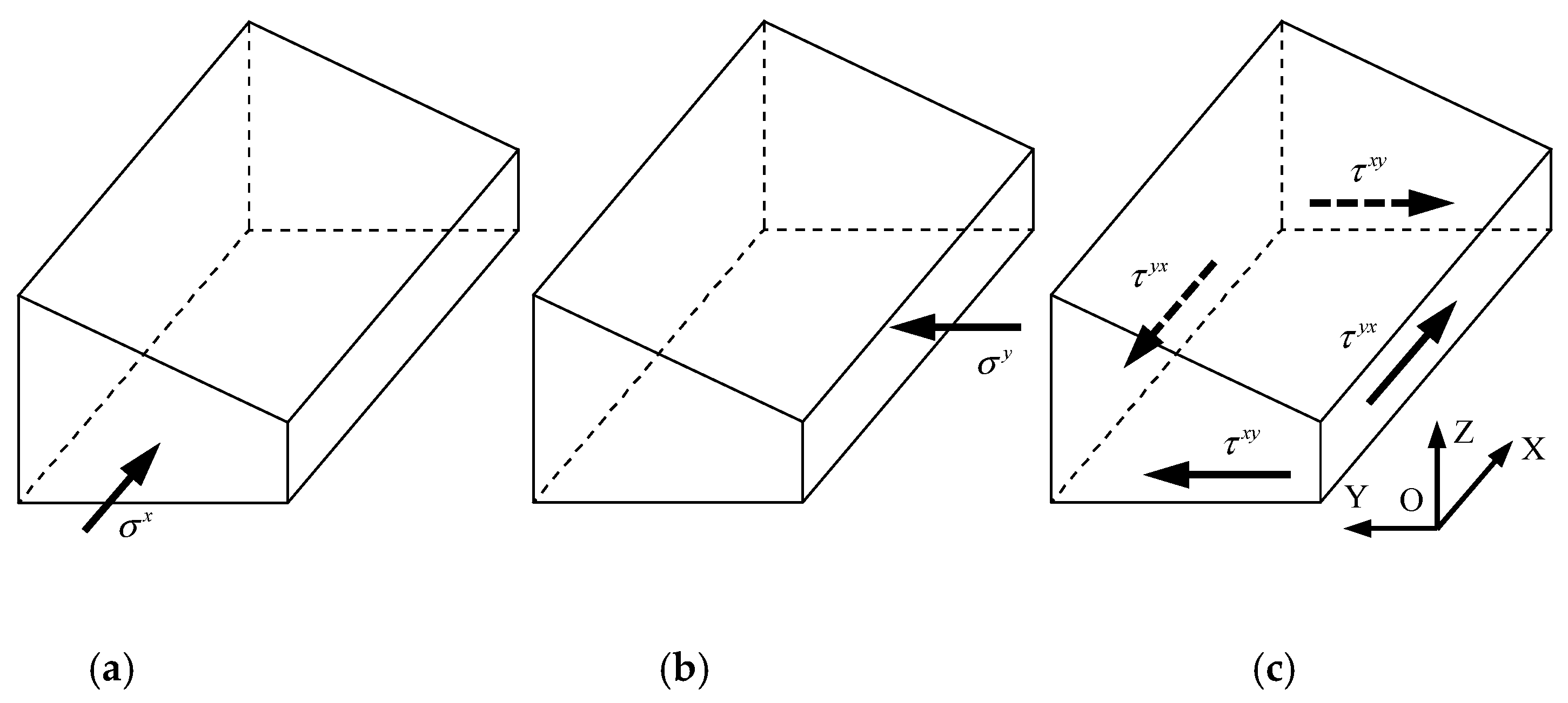
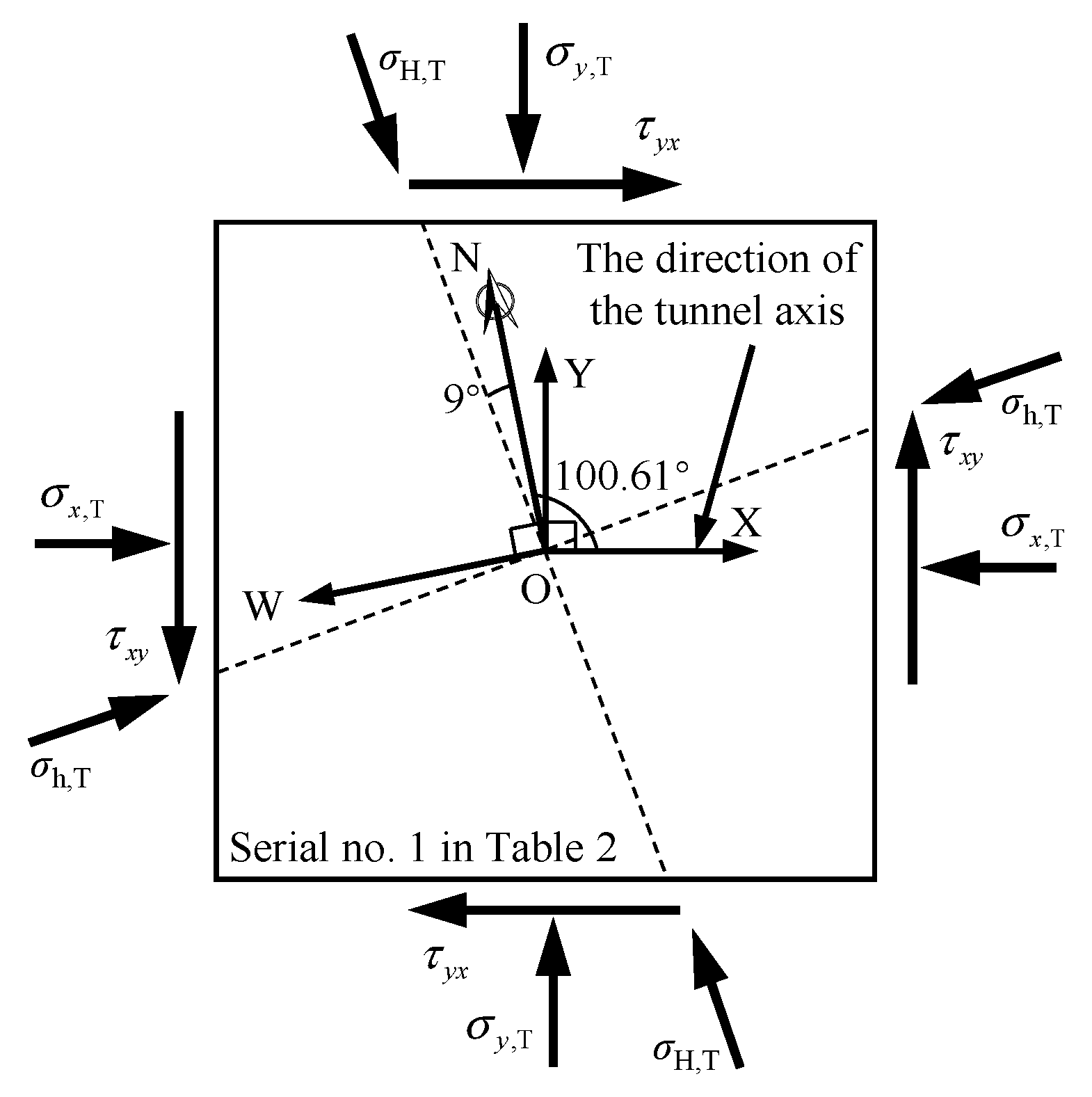
5.4. Transforming the Coordinate of in Situ Stresses
5.5. Removing Gravitational and Thermal Stresses
5.6. Solving Regression Coefficients and Superposing Stress Fields
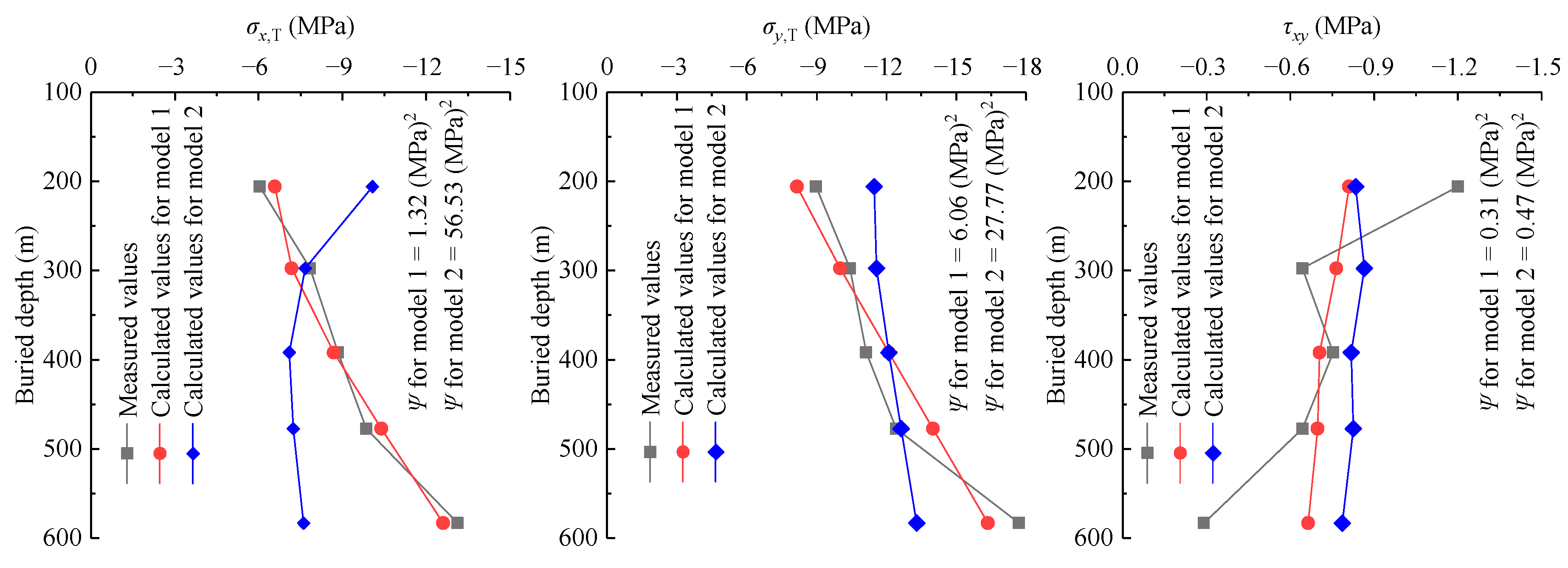
5.7. Discussion
6. Conclusions
- (1)
- Since the vertical stresses that are measured by the hydraulic fracturing method contain only gravitational information in a high geo-temperature environment, if stresses are measured by the hydraulic fracturing method, the regression coefficient of the gravitational stress field of rock masses should be set to one during a back analysis.
- (2)
- In a high geo-temperature environment, the vertical stresses that are measured by overcoring methods contain not only gravitational information, but also the information of stresses caused by geo-temperature, weathering, deposition, erosion, or tectonism. Therefore, is introduced to reflect the information of stresses caused by weathering, deposition, erosion, or tectonism during a back analysis. That is, if stresses are measured by overcoring methods, the regression coefficient of the gravitational stress field of rock masses will not be equal to one during a back analysis.
- (3)
- Based on the information of measured vertical stresses, a workflow for the back analysis of the initial geo-stress field of rock masses considering geo-temperature is proposed (see Figure 4), and this workflow can obtain the initial geo-stress field that is more compatible with the measured in situ stress of rock masses.
- (4)
- In the Sangzhuling tunnel, since in situ stresses were measured by the hydraulic fracturing method, only tectonic stress fields need to be inversely determined.
- (5)
- In this study, the thermal stress field of the same stratum was discussed. However, actual rock masses contain different strata. Therefore, the thermal stress field of different strata will need to be investigated in the future.
Author Contributions
Funding
Conflicts of Interest
References
- Wang, M.N.; Hu, Y.P.; Wang, Q.L.; Tian, H.T.; Liu, D.G. A study on strength characteristics of concrete under variable temperature curing conditions in ultra-high geothermal tunnels. Constr. Build. Mater. 2019, 229, 116989. [Google Scholar] [CrossRef]
- Cui, S.G.; Liu, P.; Cui, E.Q.; Su, J.; Huang, B. Experimental study on mechanical property and pore structure of concrete for shotcrete use in a hot-dry environment of high geothermal tunnels. Constr. Build. Mater. 2018, 173, 124–135. [Google Scholar] [CrossRef]
- Hu, Y.P.; Wang, M.N.; Wang, Q.L.; Liu, D.G.; Tong, J.J. Field test of thermal environment and thermal adaptation of workers in high geothermal tunnel. Build. Environ. 2019, 160, 106174. [Google Scholar]
- Haimson, B.C.; Cornet, F.H. ISRM Suggested Methods for rock stress estimation—Part 3: Hydraulic fracturing (HF) and/or hydraulic testing of pre-existing fractures (HTPF). Int. J. Rock Mech. Min. Sci. 2003, 40, 1011–1020. [Google Scholar] [CrossRef]
- Sjöberg, J.; Christiansson, R.; Hudson, J.A. ISRM suggested methods for rock stress estimation—Part 2: Overcoring methods. Int. J. Rock Mech. Min. Sci. 2003, 40, 999–1010. [Google Scholar] [CrossRef]
- Yang, S.X.; Huang, L.Y.; Xie, F.R.; Cui, X.F.; Yao, R. Quantitative analysis of the shallow crustal tectonic stress field in China mainland based on in situ stress data. J. Asian Earth Sci. 2014, 85, 154–162. [Google Scholar] [CrossRef]
- Meng, W.; Chen, Q.C.; Zhao, Z.; Wu, M.L.; Qin, X.H.; Zhang, C.Y. Characteristics and implications of the stress state in the Longmen Shan fault zone, eastern margin of the Tibetan Plateau. Tectonophysics 2015, 656, 1–19. [Google Scholar] [CrossRef]
- Meng, W.; Chen, Q.C.; Wu, M.L.; Feng, C.J.; Qin, X.H. Tectonic stress state changes before and after the Wenchuan Ms 8.0 earthquake in the eastern margin of the Tibetan Plateau. Acta Geol. Sin. (Engl. Ed.) 2015, 89, 77–89. [Google Scholar]
- Meng, W.; Guo, C.B.; Zhang, Y.S.; Du, Y.B.; Zhang, M.; Bao, L.H.; Zhang, P. In Situ Stress Measurements in the Lhasa Terrane, Tibetan Plateau, China. Acta Geol. Sin. (Engl. Ed.) 2016, 90, 2022–2035. [Google Scholar]
- Ju, W.; Sun, W.F.; Ma, X.J. Tectonic stress pattern in the Chinese Mainland from the inversion of focal mechanism data. J. Earth Syst. Sci. 2017, 126, 41. [Google Scholar]
- Zhao, H.J.; Ma, F.S.; Xu, J.M.; Guo, J. In situ stress field inversion and its application in mining-induced rock mass movement. Int. J. Rock Mech. Min. Sci. 2012, 53, 120–128. [Google Scholar] [CrossRef]
- McKinnon, S.D. Analysis of stress measurements using a numerical model methodology. Int. J. Rock Mech. Min. Sci. 2001, 38, 699–709. [Google Scholar] [CrossRef]
- Wang, J.L.; Li, M.; Xu, S.C.; Qu, Z.H.; Jiang, B. Simulation of Ground Stress Field and Advanced Prediction of Gas Outburst Risks in the Non-Mining Area of Xinjing Mine, China. Energies 2018, 11, 1285. [Google Scholar] [CrossRef]
- Lee, H.; Ong, S.H. Estimation of In Situ Stresses with Hydro-Fracturing Tests and a Statistical Method. Rock Mech. Rock Eng. 2018, 51, 779–799. [Google Scholar] [CrossRef]
- Obara, Y.; Nakamura, N.; Kang, S.S.; Kaneko, K. Measurement of local stress and estimation of regional stress associated with stability assessment of an open-pit rock slope. Int. J. Rock Mech. Min. Sci. 2000, 37, 1211–1221. [Google Scholar] [CrossRef]
- Zhang, T.J.; Zhang, L.; Li, S.G.; Liu, J.L.; Pan, H.Y.; Song, S. Stress Inversion of Coal with a Gas Drilling Borehole and the Law of Crack Propagation. Energies 2017, 10, 1743. [Google Scholar] [CrossRef]
- Han, H.X.; Yin, S.D. Determination of In-Situ Stress and Geomechanical Properties from Borehole Deformation. Energies 2018, 11, 131. [Google Scholar] [CrossRef]
- McKinnon, S.D.; Garrido de la Barra, I. Stress field analysis at the El Teniente Mine: Evidence for N–S compression in the modern Andes. J. Struct. Geol. 2003, 25, 2125–2139. [Google Scholar] [CrossRef]
- Liu, C.L.; Li, G.; Kuriyama, K.; Mizuta, Y. Development of a computer program for inhomogeneous modeling using 3-D BEM with analytical integration and its application to rock slope stability evaluation. Int. J. Rock Mech. Min. Sci. 2005, 1, 137–144. [Google Scholar] [CrossRef]
- Li, G.; Mizuta, Y.; Ishida, T.; Li, H.; Nakama, S.; Sato, T. Stress field determination from local stress measurements by numerical modelling. Int. J. Rock Mech. Min. Sci. 2009, 46, 138–147. [Google Scholar] [CrossRef]
- Khademian, Z.; Shahriar, K.; Gharouni Nik, M. Developing an algorithm to estimate in situ stresses using a hybrid numerical method based on local stress measurement. Int. J. Rock Mech. Min. Sci. 2012, 55, 80–85. [Google Scholar] [CrossRef]
- Figueiredo, B.; Cornet, F.H.; Lamas, L.; Muralha, J. Determination of the stress field in a mountainous granite rock mass. Int. J. Rock Mech. Min. Sci. 2014, 72, 37–48. [Google Scholar] [CrossRef]
- Zhang, S.R.; Hu, A.K.; Wang, C. Three-dimensional inversion analysis of an in situ stress field based on a two-stage optimization algorithm. J. Zhejiang Univ.-Sci. A 2016, 17, 782–802. [Google Scholar] [CrossRef]
- Pei, Q.T.; Ding, X.L.; Liu, Y.K.; Lu, B.; Huang, S.L.; Fu, J. Optimized back analysis method for stress determination based on identification of local stress measurements and its application. Bull. Eng. Geol. Environ. 2019, 78, 375–396. [Google Scholar] [CrossRef]
- Zhang, C.Q.; Feng, X.T.; Zhou, H. Estimation of in situ stress along deep tunnels buried in complex geological conditions. Int. J. Rock Mech. Min. Sci. 2012, 52, 139–162. [Google Scholar] [CrossRef]
- Li, F.; Wang, J.A.; Brigham, J.C. Inverse calculation of insitu stress in rock mass using the Surrogate-Model Accelerated Random Search algorithm. Comput. Geotech. 2014, 61, 24–32. [Google Scholar] [CrossRef]
- Li, Y.S.; Yin, J.M.; Chen, J.P.; Xu, J. Analysis of 3D In-situ Stress Field and Query System’s Development Based on Visual BP Neural Network. Procedia Earth Planet. Sci. 2012, 5, 64–69. [Google Scholar]
- Shi, Y.L.; Marcelo, A. Genetic Algorithm-Finite Element Inversion of Stress Field of Brazil. Chin. J. Geophys. 2000, 43, 191–199. [Google Scholar] [CrossRef]
- Song, Z.F.; Sun, Y.J.; Lin, X. Research on In Situ Stress Measurement and Inversion, and its Influence on Roadway Layout in Coal Mine with Thick Coal Seam and Large Mining Height. Geotech. Geol. Eng. 2018, 36, 1907–1917. [Google Scholar]
- Wang, Q.W.; Ju, N.P.; Du, L.L.; Huang, J.; Hu, Y. Three dimensional inverse analysis of geostress field in the Sangri–Jiacha section of Lasa–Linzhi railway. Rock Soil Mech. 2018, 39, 1450–1462. [Google Scholar]
- Huang, S.L.; Ding, X.L.; Liao, C.G.; Wu, A.Q.; Yin, J.M. Initial 3D geostress field recognition of high geostress field at deep valley region and considerations on underground powerhouse layout. Chin. J. Rock Mech. Eng. 2014, 33, 2210–2224. [Google Scholar]
- Yu, X.F.; Zheng, Y.R.; Liu, H.H.; Fang, Z.C. Stability Analysis of Surrounding Rock Mass in Underground Engineering; Coal Industry Press: Beijing, China, 1983; pp. 51–52. [Google Scholar]
- Zheng, Y.R.; Zhu, H.H.; Fang, Z.C.; Liu, H.H. The Stability Analysis and Design Theory of Surrounding Rock of Underground Engineering; China Communications Press: Beijing, China, 2012; pp. 17–21. [Google Scholar]
- Zhang, Y.M.; Chang, J.; Liu, N.; Liu, J.W.; Ma, X.F.; Zhao, S.F.; Shen, F.Y.; Zhou, Y. Present-day temperature–pressure field and its implications for the geothermal resources development in the Baxian area, Jizhong Depression of the Bohai Bay Basin. Nat. Gas Ind. B 2018, 5, 226–234. [Google Scholar] [CrossRef]
- Wang, L.S.; Li, C.; Liu, S.W.; Li, H.; Xu, M.J.; Wang, Q.; Ge, R. Characteristics of Geo-Temperature Gradient Distribution in the Kuqa Foreland Basin on the North Edge of the Tarim Basin, Western China. Chin. J. Geophys. 2003, 46, 575–581. [Google Scholar] [CrossRef]
- Zhan, F.L.; Cai, M.F. Influence of Earth Temperature Gradient on Ground Stress Calculation in Underground Mines. Min. Res. Dev. 2006, 26, 24–25, 48. [Google Scholar]
- Leeman, E.R. The determination of the complete state of stress in rock in a single borehole—Laboratory and underground measurements. Int. J. Rock Mech. Min. Sci. Geomech. Abstr. 1968, 5, 31–38. [Google Scholar] [CrossRef]
- Hochstein, M.P.; Regenauer-Lieb, K. Heat generation associated with collision of two plates: The Himalayan geothermal belt. J. Volcanol. Geotherm. Res. 1998, 83, 75–92. [Google Scholar] [CrossRef]
- Zhang, X.B.; Hu, Q.H. Development of Geothermal Resources in China: A Review. J. Earth Sci. 2018, 29, 452–467. [Google Scholar] [CrossRef]
- Yokoyama, T.; Nakai, S.I.; Wakita, H. Helium and carbon isotopic compositions of hot spring gases in the Tibetan Plateau. J. Volcanol. Geotherm. Res. 1999, 88, 99–107. [Google Scholar] [CrossRef]
- Yan, J.; He, C.; Wang, B.; Meng, W.; Wu, F.Y. Inoculation and characters of rockbursts in extra-long and deep-lying tunnels located on Yarlung Zangbo suture. Chin. J. Rock Mech. Eng. 2019, 38, 769–781. [Google Scholar]
- Yan, J.; He, C.; Wang, B.; Meng, W.; Yang, J.F. Prediction of Rock Bursts for Sangzhuling Tunnel Located on Lhasa-Nyingchi Railway Under Coupled Thermo-Mechanical Effects. J. Southwest Jiaotong Univ. 2018, 53, 434–441. [Google Scholar]
- Zhao, B. GPS Velocity Field of CMONOC with Respect to Eurasia. 2015. Available online: ftp://ftp.cgps.ac.cn/products/velocity/image/cmnc_vel_eura_grd_flt.png (accessed on 5 September 2019).


| Rock Matrix | Elastic Modulus (GPa) | Poisson’s Ratio | Density (kg/m3) | Thermal Expansion Coefficient (°C−1) |
|---|---|---|---|---|
| Diorite | 36 | 0.20 | 2600 | |
| Rubble soil | 0.1 | 0.38 | 2300 |
| Serial No. | Buried Depth (m) | (MPa) | (MPa) | (MPa) | |
|---|---|---|---|---|---|
| 1 | 205.85 | −9.41 | −5.61 | −4.92 | |
| 2 | 297.70 | −10.58 | −7.70 | −7.31 | () |
| 3 | 392.10 | −11.36 | −8.61 | −9.76 | |
| 4 | 477.20 | −12.58 | −9.70 | −11.98 | () |
| 5 | 582.85 | −17.72 | −13.10 | −14.72 |
| Serial No. | (MPa) | (MPa) | (MPa) | (MPa) |
|---|---|---|---|---|
| 1 | −6.04 | −8.98 | −4.92 | −1.20 |
| 2 | −7.85 | −10.43 | −7.31 | −0.64 |
| 3 | −8.83 | −11.14 | −9.76 | −0.75 |
| 4 | −9.85 | −12.43 | −11.98 | −0.64 |
| 5 | −13.12 | −17.70 | −14.72 | −0.29 |
| Serial No. | (MPa) | (MPa) | (MPa) |
|---|---|---|---|
| 1 | −3.82 | −6.77 | −1.20 |
| 2 | −3.58 | −6.16 | −0.64 |
| 3 | −2.46 | −4.76 | −0.75 |
| 4 | −1.57 | −4.15 | −0.64 |
| 5 | −2.48 | −7.06 | −0.29 |
| Magnitudes and Orientations | Buried Depth (m) | Residual Sum of Squares | |||||
|---|---|---|---|---|---|---|---|
| 205.85 | 297.7 | 392.1 | 477.2 | 582.85 | |||
| (MPa) | Measured values | −6.04 | −7.85 | −8.83 | −9.85 | −13.12 | |
| Calculated values for model 1 | −6.58 | −7.18 | −8.69 | −10.40 | −12.60 | ||
| Calculated values for model 2 | −10.07 | −7.67 | −7.09 | −7.25 | −7.60 | ||
| Residuals for model 1 | 0.54 | −0.67 | −0.14 | 0.54 | −0.51 | 1.32 | |
| Residuals for model 2 | 4.03 | −0.18 | −1.74 | −2.60 | −5.51 | 56.53 | |
| (MPa) | Measured values | −8.98 | −10.43 | −11.14 | −12.43 | −17.70 | |
| Calculated values for model 1 | −8.17 | −10.00 | −12.11 | −14.01 | −16.37 | ||
| Calculated values for model 2 | −11.46 | −11.57 | −12.11 | −12.63 | −13.31 | ||
| Residuals for model 1 | −0.82 | −0.42 | 0.98 | 1.58 | −1.33 | 6.06 | |
| Residuals for model 2 | 2.48 | 1.14 | 0.98 | 0.21 | −4.39 | 27.77 | |
| (MPa) | Measured values | −1.20 | −0.64 | −0.75 | −0.64 | −0.29 | |
| Calculated values for model 1 | −0.81 | −0.76 | −0.71 | −0.70 | −0.66 | ||
| Calculated values for model 2 | −0.83 | −0.86 | −0.82 | −0.83 | −0.79 | ||
| Residuals for model 1 | −0.39 | 0.12 | −0.05 | 0.05 | 0.37 | 0.31 | |
| Residuals for model 2 | −0.37 | 0.22 | 0.06 | 0.18 | 0.50 | 0.47 | |
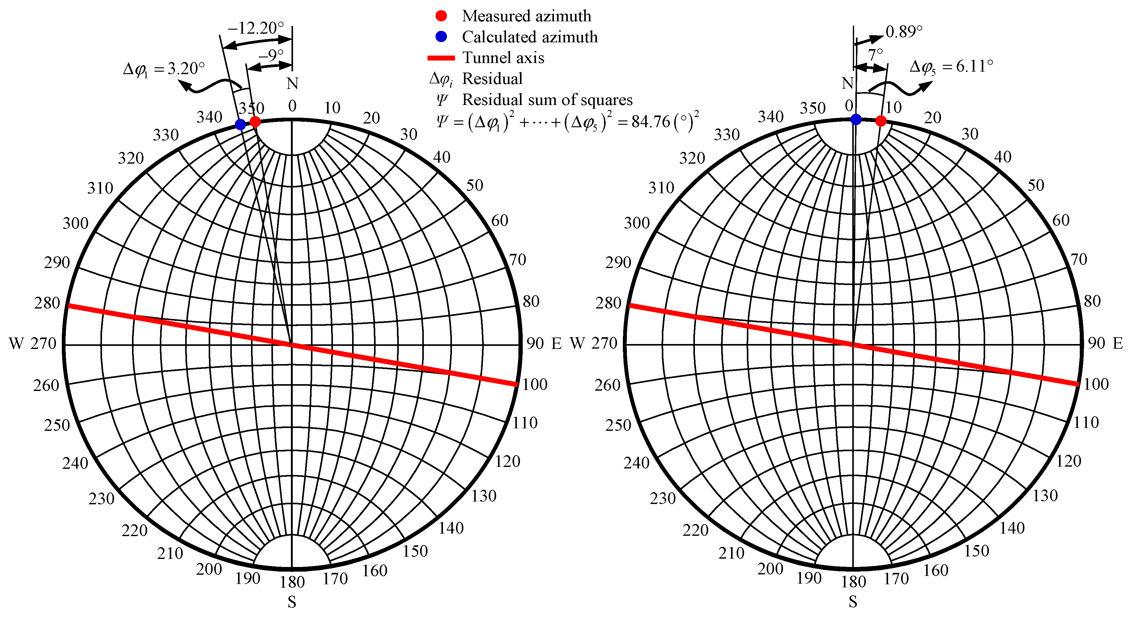
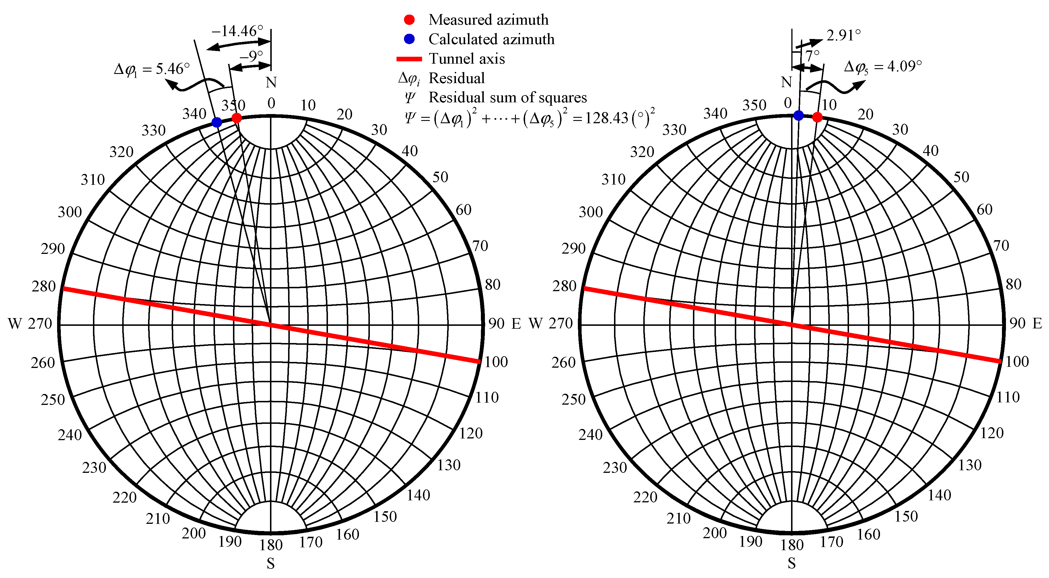
| (°) | Measured values | −9 | −2.67 | −6 | −2.67 | 7 | |
| Calculated values for model 1 | −12.20 | −3.63 | −0.61 | 0.03 | 0.89 | ||
| Calculated values for model 2 | −14.46 | −1.36 | 1.59 | 2.08 | 2.91 | ||
| Residuals for model 1 | 3.20 | 0.96 | −5.39 | −2.70 | 6.11 | 84.76 | |
| Residuals for model 2 | 5.46 | −1.31 | −7.59 | −4.75 | 4.09 | 128.43 | |
© 2020 by the authors. Licensee MDPI, Basel, Switzerland. This article is an open access article distributed under the terms and conditions of the Creative Commons Attribution (CC BY) license (http://creativecommons.org/licenses/by/4.0/).
Share and Cite
Meng, W.; He, C. Back Analysis of the Initial Geo-Stress Field of Rock Masses in High Geo-Temperature and High Geo-Stress. Energies 2020, 13, 363. https://doi.org/10.3390/en13020363
Meng W, He C. Back Analysis of the Initial Geo-Stress Field of Rock Masses in High Geo-Temperature and High Geo-Stress. Energies. 2020; 13(2):363. https://doi.org/10.3390/en13020363
Chicago/Turabian StyleMeng, Wei, and Chuan He. 2020. "Back Analysis of the Initial Geo-Stress Field of Rock Masses in High Geo-Temperature and High Geo-Stress" Energies 13, no. 2: 363. https://doi.org/10.3390/en13020363
APA StyleMeng, W., & He, C. (2020). Back Analysis of the Initial Geo-Stress Field of Rock Masses in High Geo-Temperature and High Geo-Stress. Energies, 13(2), 363. https://doi.org/10.3390/en13020363