Abstract
The power capacity of solar photovoltaics (PVs) in Korea has grown dramatically in recent years, and an accurate estimation of solar resources is crucial for the efficient management of these solar PV systems. Since the number of solar irradiance measurement sites is insufficient for Korea, satellite images can be useful sources for estimating solar irradiance over a wide area of Korea. In this study, an artificial neural network (ANN) model was constructed to calculate hourly global horizontal solar irradiance (GHI) from Korea Communication, Ocean and Meteorological Satellite (COMS) Meteorological Imager (MI) images. Solar position variables and five COMS MI channels were used as inputs for the ANN model. The basic ANN model was determined to have a window size of five for the input satellite images and two hidden layers, with 30 nodes on each hidden layer. After these ANN parameters were determined, the temporal and spatial applicability of the ANN model for solar irradiance mapping was validated. The final ANN ensemble model, which calculated the hourly GHI from 10 independent ANN models, exhibited a correlation coefficient (R) of 0.975 and root mean square error (RMSE) of 54.44 W/m² (12.93%), which were better results than for other remote-sensing based works for Korea. Finally, GHI maps for Korea were generated using the final ANN ensemble model. This COMS-based ANN model can contribute to the efficient estimation of solar resources and the improvement of the operational efficiency of solar PV systems for Korea.
1. Introduction
In Korea, solar energy is emerging as a clean and sustainable energy resource, with its biggest advantages being its ability to supply energy globally and the lack of concern over its depletion [1]. The installed capacity of solar PV in Korea has increased by more than 16 times over the last ten years, and now solar energy has become the largest renewable energy source in Korea, followed by hydropower and wind power (Figure 1). However, solar electricity production can fluctuate according to weather conditions, which hinders the stability and efficiency of PV systems. Thus, the accurate estimation and prediction of solar resources is essential to alleviate the uncertainty of solar PV systems and promote their grid penetration. This importance of solar resource estimation, however, has been overlooked in installing PV systems in Korea because of limited ground level solar irradiance data.
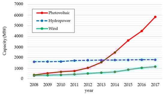
Figure 1.
Installed capacity of renewable energy sources in Korea (from kosis.kr).
Solar irradiance can be measured locally by pyranometers or sky camera images, or estimated remotely over a large region by satellite images. Pyranometers can measure solar irradiance accurately, but only over particular areas; they are also expensive to purchase and install, which limits their deployment. In this context, although Korea has 38 solar irradiance measuring stations, it is difficult to estimate solar irradiance for the entire country of Korea only by using the installed pyranometers. In order to mitigate this limitation of pyranometers, Sen and Sahin [2], Bezzi and Vitti [3], and Palmer et al. [4] used interpolation methods, such as kriging, to estimate solar irradiance for locations which have no measurement data. However, since the interpolation method assumes a static condition, the dynamic movement of clouds can add a degree of uncertainty to this method, particularly if the amount of measurement data is insufficient [5,6,7]. Although sky camera images can be used for the estimation and forecasting of solar irradiance with a better spatial and temporal resolution than satellite images [8,9,10], they are appropriate for the estimation of solar irradiance at a specific location, not for a large region [8].
Therefore, using satellite images can be an effective way to estimate solar irradiance over Korea. Using satellite images is valuable for estimating a wide range of solar irradiance with little cost and is particularly useful for mapping solar irradiance. Traditionally, two kinds of models have been used to derive solar irradiance from satellite images: physical models and empirical models [11]. Physical models use radiative transfer models, requiring complex atmospheric parameters and an accurate correction of satellite data [12]. Empirical models establish empirically derived formulas from measured solar irradiance and atmospheric parameters such as aerosol optical depth, turbidity, or precipitable water vapor [13,14]. However, these atmospheric parameters can cause significant errors in solar irradiance estimation for Korea, because observation networks of these parameters are not systematically built in Korea [15].
In recent years, in addition to these traditional approaches, the artificial neural network (ANN) has been recognized as a powerful tool for estimating solar irradiance from satellite images [16]. ANN can be a good alternative to traditional methods for the estimation of solar irradiance in Korea, because it does not require complex physical models or atmospheric parameters. Furthermore, if a sufficient amount of data is available, ANN is known to be more effective than conventional statistical methods for solving complex problems, especially when it is difficult to derive theoretical models [17]. Therefore, applying ANN can be a good choice for the estimation of solar irradiance, because solar radiation reaches the ground after making complex progress through the atmosphere, including transmission, absorption, scattering, and reflection.
Various studies have been conducted regarding the use of ANN for the estimation and prediction of solar resources from satellite images. Linares-Rodriguez et al. [16] built ANN ensemble models to estimate daily solar irradiance in Andalusia, Spain, from visible and infrared channels of the Meteosat 9. Eissa et al. [18] and Alobaidi et al. [19] used ANN ensembles to estimate solar irradiance in the United Arab Emirates (UAE), using the Spinning Enhanced Visible and Infrared Imager (SEVIRI) instrument channels onboard the Meteosat Second Generation (MSG) satellite. Quesada-Ruiz et al. [20] applied ANN ensemble models to estimate solar irradiance over northern Africa, the Middle East and Europe from the MSG satellite, and then compared the results with the conventional Heliosat-2 empirical model. Ameen et al. [21] used the ANN method to obtain solar irradiance for northeast Iraq from satellite-derived datasets, top-of-atmosphere irradiance, and observed climate variables. Marquez et al. [22] detected clouds and their velocities from satellite images, and then used them as inputs for ANN models to forecast solar irradiance at Davis and Merced, California.
In Korea, various physical, empirical and ANN methods have been suggested to calculate solar irradiance using satellite data. Yeom et al. [23] used the MTSAT-1R (Multi-Functional Transport Satellite) to derive solar irradiance from the modified physical model of Kawamura [24]. Zo et al. [25] developed the Gangneung-Wonju National University (GWNU) solar radiation model, based on MTSAT-2, MODIS (Moderate Resolution Imaging Spectroradiometer), and Ozone Monitoring Instrument (OMI) data. Zo et al. [26], Yeom et al. [27], Kim et al. [28], and Kim et al. [29] used various physical models—GWNU, Kawamura, CLAVR-x (Clouds from AVHRR Extended), and UASIBS/KIER (University of Arizona Solar Irradiance Based on Satellite/Korea Institute of Energy Research) models—to derive solar irradiance from Korea’s Communication, Ocean and Meteorological Satellite (COMS) images. In addition, Choi et al. [15] adapted the existing Heliosat-2 empirical model for application to Korea, and Yeom and Han [30] used ANN to calculate solar irradiance for Korea using MTSAT-1R satellite data. The overall accuracies of these studies are presented in Table 1, where it can be seen that the ANN method [30] has shown the best performance among other methods.

Table 1.
Previous studies on solar irradiance estimation from satellite images, in Korea. RMSE: root mean square error; ANN: artificial neural network; MTSAT-1R: Multi-Functional Transport Satellite; OMI: Ozone Monitoring Instrument; COMS: Communication, Ocean and Meteorological Satellite.
COMS and MTSAT have been used as the main satellite data sources in solar irradiance research for Korea. However, since the positions of the MTSAT geosynchronous orbits—longitude 140° E (MTSAT-1R) or 145° E (MTSAT-2)—are adjusted to Japan, its observation area is biased to the east of Korea. On the other hand, since the COMS geosynchronous orbit is at longitude 128.2° E, its observation area is adjusted for Korea (nmsc.kma.go.kr). In this regard, compared to MTSAT, using COMS satellite images can improve the solar irradiance estimation accuracy for Korea. Nevertheless, while COMS data have been used for physical or empirical solar irradiance estimation, studies that used COMS and ANN for solar irradiance derivation in Korea have not been found.
Therefore, the aim of this study is to improve the solar irradiance estimation accuracy for Korea by building an ANN model using COMS satellite data. In order to improve the performance of the ANN, the basic structure of the ANN model was determined by changing training parameters, including the extent of input satellite data, the number of hidden layers, and the number of nodes in each hidden layer. Then, after validating the applicability and generality of the ANN model for solar irradiance mapping, the final ANN model was trained and evaluated. This final ANN model was used to produce solar irradiance maps of Korea, so that the solar irradiance over Korea was estimated.
2. Study Area and Data Collection
The study area is the territory of Korea, which has an area of 100,200 km². Korea is located between 33°–39° N and 124°–130° E and is surrounded by the sea on three sides. There are many mountains in its east, and many small islands in the west and south. Korea has four distinct seasons: spring, summer, autumn, and winter. Over the year, 50–60% of precipitation falls in the summer months of June–August, and snow sometimes falls during the winter months of December–February.
COMS satellite images were used as ANN input data. COMS is the first geostationary satellite made by Korea, and it was launched in 2010 for the purpose of monitoring meteorological phenomena and the environment. Its orbit is geosynchronous at the Earth’s equator, at 128.2° E, at an altitude of 36,000 km. Its meteorological imager (MI) has five channels: visible (VIS), shortwave infrared (SWIR), water vapor (WV), infrared 1 (IR1), and infrared 2 (IR2). It produces images every 15 min. Detailed information for each channel is presented in Table 2.
Table 2.
COMS MI channel information (nmsc.kma.go.kr).
Solar irradiance measurement data are also necessary to train and test the ANN model. The Korea Meteorological Administration (KMA) has been measuring global horizontal solar irradiance (GHI) at 38 automated synoptic observing system (ASOS) weather stations throughout Korea. The recorded GHI values are accumulative values for an hour. In this study, data from some stations were excluded as they showed a significant decline or discontinuity of GHI values in recent years compared to the previous 10 years. The stations that showed a dramatic and discontinuous reduction of daily maximum GHI—by more than 200 Wh/m² in 2016 and 2017—were excluded. Since the sudden decrease pattern in the daily maximum GHI values they recorded is physically impossible, it must have been due to measurement errors caused by sensor degradation. As a result, data from 25 stations were selected and used (Figure 2). These COMS MI images and ground GHI measurement data were acquired for 2016–2017.
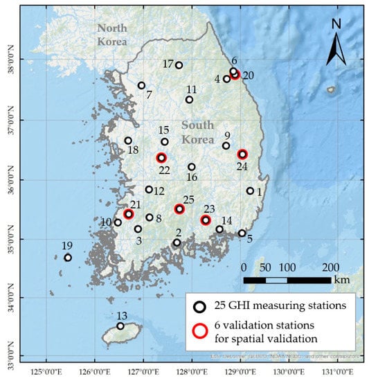
Figure 2.
The location of selected weather stations in Korea. GHI: global horizontal solar irradiance.
3. Methodology
3.1. Data Preprocessing
The overall process of this study is described in Figure 3. Before training the ANN model and determining its construction parameters, the data should be preprocessed to exclude invalid data and to transform raw input data into the form required for ANN training. Such data preprocessing can help us to achieve the best analysis results, while addressing some of the issues caused by managing a large amount of information [31].
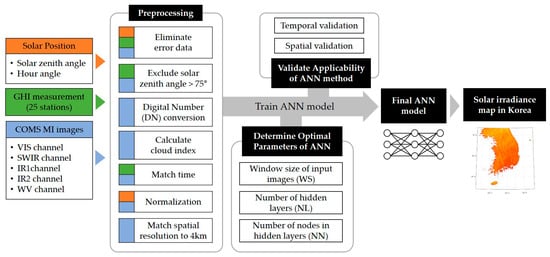
Figure 3.
The flow chart of overall process.
The first preprocessing step was to remove physically problematic GHI measurement data. Although solar irradiance observation data are measured by automatic systems, errors can occur through faulty sensors or systems. As an example of this error, if the data shows a zero GHI value even when the sun is at a high elevation in a cloudless sky, it would be reasonable to consider that the zero reading was an error from a sensor or from the system, because the solar radiation value should be positive. The factors for identifying the existence of this type of error were the solar zenith angle (z) and the amount of cloud. The solar zenith angle, the angle of the sun from the zenith of the sky, can be calculated using the time and geographical location. The amount of cloud can be quantified using the cloud index (CI) derived from COMS visible channel images. A lower CI value means fewer clouds, while a higher CI means a larger amount of clouds; thus, the CI can be used to distinguish clear skies from cloudy skies. The CI for pixel , at time t, is calculated using Equation (1) [32].
where is the visible channel reflectance on pixel at time t, is the reflectance of the ground, and is the reflectance of the cloud. is the maximum reflectance in a time series of 30 days, and is the second minimum reflectance in the same time series. The second minimum reflectance is used as to remove outliers, which can be caused by cloud shadow or the sun being above the horizon [14,33]. Consequently, GHI measurements showing zero when CI < 0.1 and cosine of z > 0.1 were removed, on the basis that they were sensor or system errors.
The next preprocessing step was to transform and match the data. In this study, two types of variables—solar position and satellite data—were used as ANN input data. Since the purpose of this study is to derive solar irradiance by the data-based training of raw satellite images, we do not consider external products, such as air pressure, elevation, or temperature, as ANN inputs. Solar position variables contain the solar zenith angle and hour angle, and satellite variables contain images of five COMS MI channels. All these input data were normalized to have the same range [0, 1], because different units and scales of data can cause errors in the initialization and adjustment of ANN weights [34]. When several normalized ranges for input data were tested, a range of [0, 1] showed the best result for our ANN model. The solar zenith angle was normalized by transforming it to a cosine value, but the other data were linearly normalized by Equation (2).
where is the minimum value of the data, and is the maximum value.
The solar zenith angle and hour angle were calculated from the time and location of the data. The hour angle () means the angular displacement of the sun with respect to zero when the sun is in a southernly direction [35]. It was normalized by considering the hour angles of sunset as , and sunrise as , in Equation (2) [36].
Satellite data were processed by using several methods before normalization. First, the digital number (DN) of the raw satellite data (0–1023) was converted into radiance or brightness temperature, according to the conversion table provided by the KMA National Meteorological Satellite Center (nmsc.kma.go.kr). Next, since the spatial resolution of the visible channel was different (1 km) to that of the other channels (4 km), visible channel data were resampled to have a resolution of 4 km.
Another issue was that measured GHI data were provided as hourly cumulative values, whereas satellite data were provided as instantaneous values. In order to match the ground measurement and satellite data timing, the mean value of measured GHI for the previous and next one hour was considered as the instant GHI value at the satellite image acquisition time. In addition, since the physical estimation of solar irradiance from satellite data can be invalid when the solar elevation is <15° [14], data were excluded when the solar zenith angle was >75°. After the available data were filtered, the total number of data points used in this study was 161,105.
3.2. Design of ANN
The construction of the ANN model in this study is based on the multilayer perceptron (MLP), which is a simple and general form of ANN [37,38,39]. MLP generally consists of an input layer, one or more hidden layers, and an output layer. Nodes in each layer are fully connected to the other nodes in the next layer with weights, biases, and activation functions. For each layer, input signals from previous nodes are transferred to node k as described in Equation (3) [37,38].
where are the input signals to node k in a layer, are the respective synaptic weights, is the bias of node k, is the output signal of the node, and is the activation function.
MLP is trained by the back-propagation algorithm, and training proceeds in two phases: forward and backward computation [37]. In this study, for each training cycle, weights and biases are updated by using the Levenberg–Marquardt optimization algorithm [40]. This method combines the feature of the Gauss–Newton algorithm and gradient descent method [41], and minimizes a linear combination of squared errors and weights [16]. Since it is rapid and appropriate to avoid falling into a local minimum, it has been utilized in many real applications [16,41,42,43]. The hyperbolic tangent function in Equation (4), which showed the best result for our ANN model among various activation functions, was used as an activation function.
Since the weight and bias are randomly initialized, the results can vary with each training cycle. Thus, in order to minimize this fluctuant effect and improve the accuracy of solar irradiance estimation, we applied the ANN ensemble, which has been used for ANN-based solar irradiance mapping [16,18,19]. Our ANN ensemble model consisted of 10 independent ANN models, and the final GHI value was the average of the outputs from the 10 models. The building and training of ANN models was conducted using the Neural Network Toolbox in MATLAB R2018a software (MathWorks, MA, USA).
3.3. Determination of ANN Parameters
In order to improve accuracy, the basic parameters of the ANN model were determined using a trial and error approach. Accuracy was calculated by changing the three parameters of the window size of the input satellite images (WS), the number of hidden layers (NL), and the number of nodes in each hidden layer (NN). For this ANN parameter determination process, data for 2016 (number of data points = 82,679) were used for training and data for 2017 (number of data points = 78,426) were used for testing.
WS is the width of the satellite image that was to be used as input. A WS of 1 refers to the use of one exact pixel, and an increase of the WS means the use of additional nearby pixels. WS 3 uses nine nearby pixels, and WS 5 uses 25 (Figure 4). Since the sun is not always in the vertical position, it is necessary to identify surrounding clouds to consider their shadows. Using nearby pixels means that these surrounding clouds can be considered. For example, when using WS 5, it is possible to consider a cloud at an approximately 8 km distance. This means that when the height of the cloud is 10 km, it is possible to consider cloud shadow up to approximately 40° of the solar zenith angle (Figure 4). The larger the WS, the wider the range that can be considered, but the amount of data exponentially increases. Therefore, considering model efficiencies, WSs of 1, 3, and 5 were analyzed in this study.
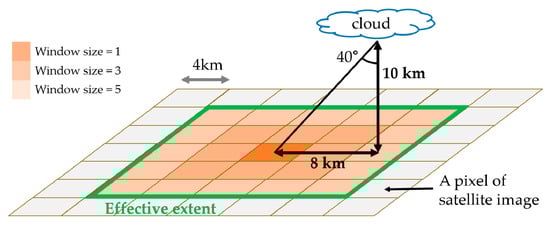
Figure 4.
Illustration of the effective extent.
The other two parameters, the number of hidden layers (NL) and number of nodes in hidden layers (NN), are crucial in determining the ANN’s capability to learn and generalize [44]. Although a number of methods have been proposed to determine these hidden layer parameters, there are no generally accepted methods, so trial and error has mainly been used [44,45]. Thus, in this study, optimal values were found by comparing results from many different cases: NLs from 1–4, in intervals of one, and NNs from 15–40, in intervals of five. All hidden layers had the same number of nodes. A total of 24 cases—four NLs with six NN cases—were therefore calculated and analyzed.
The accuracy was evaluated by the correlation coefficient (R) and root mean square error (RMSE). R is defined by Equation (5), and RMSE is defined by Equation (6). R has a range from −1 to 1. A positive R value means that the estimation and measurement data have a positive correlation, and a negative R means negative correlation. Therefore, the closer the value of R is to 1, the greater the accuracy of the model. With the absolute RMSE derived by Equation (6), the relative RMSE (rRMSE) was also used, which can be obtained by Equation (7). The unit of RMSE is the same as that of the original value (W/m²), while the unit of rRMSE is percentage (%); a lower RMSE value corresponds to better model performance.
In Equations (5) to (7), and are the hourly measured and estimated GHI (W/m²), and n is the total number of the data points. is the mean of hourly measured GHI, and is the mean of hourly estimated GHI.
3.4. Validation of ANN Applicability
After determining the optimal structure of ANN, its applicability for estimating and mapping solar resources was validated by two criteria: temporal validation and spatial validation (Figure 3). Since the purpose of this ANN model is mapping solar irradiance for Korea, the model should be able to estimate solar irradiance for any time and everywhere in Korea, with little bias. Therefore, before training and applying the final ANN model, we confirmed whether the ANN method can be applied to achieve this purpose.
First, temporal validation was performed to confirm the temporal applicability of the ANN method. An ANN model was trained using the 2016 dataset and was applied to the 2017 dataset. If the train accuracy by 2016 data is similar to the test accuracy by 2017 data, it can be said that the ANN method has temporal reliability and generality regardless of the data period.
For the spatial validation of ANN method, GHI measuring stations were divided into a test set and a train set. Considering the spatial distribution of the stations, six stations—Gangneung, Daejeon, Choengsong, Gochang-gun, Hamyang, and Uiryeong—were selected as the test set (Figure 2), and the other 19 sites were set as the train set. Then, another ANN model was trained using data from the train set and was applied to the test set. If the test accuracy showed little difference with the train accuracy, this implied that the ANN method can be used to estimate solar irradiance throughout Korea, regardless of the data location.
3.5. Solar Irradiance Mapping
At the end of this study, the final ANN model was trained and evaluated. This final ANN model, based on COMS images, was used to generate hourly solar irradiance (GHI) maps in Korea for 2016–2017. The GHI maps had a spatial resolution of 4 km, and the time interval between each map was one hour. When satellite images for a specific time were missing, the results for that time were calculated using interpolation. If there were results from one hour before and after, the median was used, and if not, the medians from the previous and next days were used. In addition, since data for a solar altitude of 15° or less were excluded in the model training, a zero GHI value was assigned when the solar altitude was less than 15°.
4. Construction of ANN model
The rRMSE values for the training and test sets by basic ANN construction parameters are shown in Figure 5. In order to analyze rRMSE variations in terms of WS, an ANN consisting of one hidden layer with 15 nodes was used. As the WS increased, the rRMSE tended to decrease (Figure 5a,b). When the WS was 5, the model showed the lowest rRMSEs in both the training and test datasets: 14.34% and 13.65%, respectively. Thus, WS = 5 was selected as the optimal value, considering the slope change and computation efficiency.
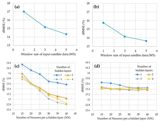
Figure 5.
rRMSE of models with various ANN construction parameters; (a) rRMSE in the training set according to the width of the satellite image (WS) (NN = 15, NL = 1), (b) rRMSE in the test set according to WS (NN = 15, NL = 1), (c) rRMSE in the training set according to NL and NN (WS = 5), (d) rRMSE in test set according to NL and NN (WS = 5).
Figure 5c,d show the results according to hidden layer parameters. In Figure 5c, the rRMSE in the training set decreased as NN increased in all NL cases. For the test set (Figure 5d), however, although rRMSE decreased with the increase of NN when NL was 1, rRMSE fluctuated when NN exceeded 30 at the other NL. In terms of NL, results of multiple NL showed lower rRMSEs than the single NL, but there was little difference between NL 2 and above. Thus, the NL and NN were determined to be 2 and 30, respectively. The ANN model shows the best performance with this NN and NL, but it is likely to show unstable accuracy and over-fitting patterns when these parameters become larger. As a result, the final ANN had the structure of WS = 5, NL = 2, and NN = 30, as illustrated in Figure 6.
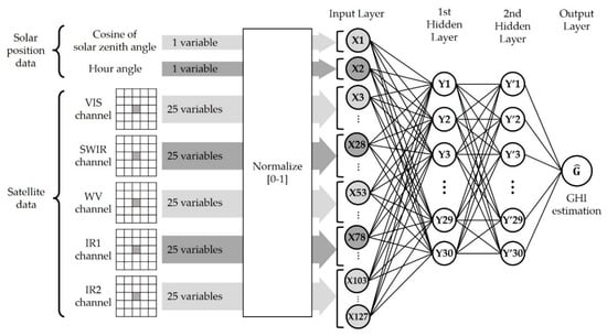
Figure 6.
Final structure of the ANN model.
5. Validation of ANN for Solar Mapping
5.1. Temporal Validation
In order to validate the temporal reliability of the ANN method for solar irradiance mapping, an ANN model was trained with the 2016 dataset (number of data = 82,679) and tested with the 2017 dataset (number of data = 78,426). The measured and estimated GHI scatter plots for each dataset are shown in Figure 7. The 2016 training dataset showed an R of 0.976 and RMSE of 53.11 W/m² (rRMSE 13.08%), while the 2017 test dataset showed an R of 0.971 and RMSE of 58.49 W/m² (rRMSE 13.39%). Since the rRMSE difference between them was negligible (0.31%), it could be concluded that this COMS-based ANN method had little time-specificity to be confidently applied to solar resource mapping in Korea for 2016 and 2017.
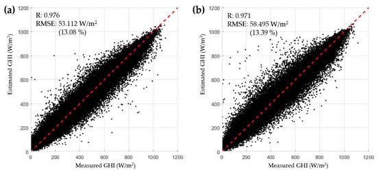
Figure 7.
Result of the temporal validation of the ANN model for (a) the train dataset (2016), (b) the test dataset (2017).
Monthly accuracy variation was also demonstrated, as shown in Table 3 and Figure 8. Summer showed a higher RMSE than other months, and this was most apparent in July and August—the rainy season in Korea. Since estimation errors generally increase in a cloudy sky [16,18,19,42], the rainy season showed relatively large errors. January also showed relatively low R and large RMSE values compared to other months, and this might have been caused by the cloud confusion effect from snow. Ground covered by snow shows high reflectance in visible and near infrared channels [46], which can cause snow cover to be confused with clouds. This anomaly can reduce accuracy for January—the month with the most snow in Korea. In 2016 and 2017, January showed the deepest snow cover of 7.4 cm and 5.5 cm on average, respectively (kosis.kr). Although the error of the model increased at times of rain or snow, the value of R was at least 0.939 or more, and the RMSE was as low as 68.86 W/m² (rRMSE 16.36%) or less every month. This level of monthly accuracy can be expected whenever the ANN method is applied to solar irradiance mapping for Korea.
Table 3.
Monthly accuracy of the temporal validation of the ANN model.
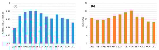
Figure 8.
Monthly accuracy of the temporal validation of the ANN model represented by (a) R and (b) rRMSE (%).
5.2. Spatial Validation
In order to validate the spatial reliability of the ANN model, another ANN model was trained using the data from 19 stations (number of data = 122,669) and applied to the data from the remaining six stations (number of data = 38,436). Table 4 and Figure 9 show the accuracy of each station. Differences of the average R and RMSE (rRMSE) between the training and test sites were 0.002 and 9.34 W/m² (1.71%p), respectively. This result indicates that, if some sites are not included in the training of the ANN model, the errors of solar irradiance estimation for these sites can be larger than the included sites, but the RMSE values were likely to increase only up to ~2%. Thus, ANN model can have significant power in solar irradiance mapping for any site in Korea, within an error range of ~15%.
Table 4.
Accuracy of the spatial validation of the ANN model for each weather station.
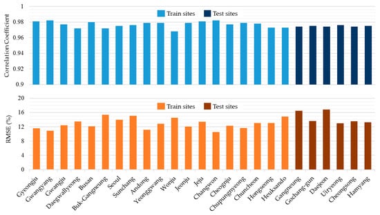
Figure 9.
Accuracy (R and rRMSE) of the spatial validation of theANN model for each weather station.
6. Application of Final ANN model
6.1. Final ANN Model
The final ANN ensemble model for solar irradiance mapping in Korea was built by averaging the outputs of 10 independent ANN models, which were trained by randomly setting the training ratio to 70% (number of data points = 112,773) and the test ratio to 30% (number of data = 48,332). The final model showed an overall R of 0.975 and RMSE of 54.44 W/m² (rRMSE 12.93%) (Figure 10a). The training set showed an R of 0.976 and RMSE of 53.33 W/m² (rRMSE 12.67%) (Figure 10b), and the test set showed an R of 0.973 and RMSE of 56.93 W/m² (rRMSE 13.51%) (Figure 10c). Although the training set showed better accuracy than the test set, the differences were marginal: 0.003 for R, 3.6 W/m² for RMSE, and 0.84%p for rRMSE. Therefore, we concluded that this final model showed a minimal overfitting pattern.
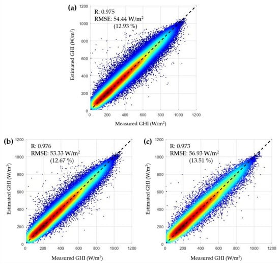
Figure 10.
Scatter plots of measured GHI and estimated GHI by the final ANN ensemble model for (a) all train and test datasets, (b) all train datasets, (c) all test datasets.
Figure 11 shows the results of estimations in different weather conditions. In clear skies, when CI < 0.2, the model showed an R of 0.974 and RMSE of 47.99 W/m² (rRMSE 11.40%). In cloudy skies, when CI > 0.2, the model showed less accuracy, with an R of 0.943 and RMSE of 60.72 W/m² (rRMSE 14.42%). Considering the significant effect of clouds on solar irradiance and its complexity, this is a reasonable consequence. Compared to MTSAT-based ANN work in Korea [30], the COMS-based ANN model of this study showed a relatively larger RMSE in clear skies by 3.13 W/m², but a lower RMSE in cloudy skies by 17.75 W/m². The COMS-based ANN model of this study showed a similar performance to MTSAT-based ANN in clear sky conditions, but much better performance for cloudy sky. This result might be because the east-biased observation area of MTSAT satellite made it difficult to estimate the impact of clouds on Korea accurately. On the other hand, in this study, the accuracy of solar irradiance estimation in cloudy skies could be improved significantly by using COMS satellite data, whose observation area is optimized for Korea.
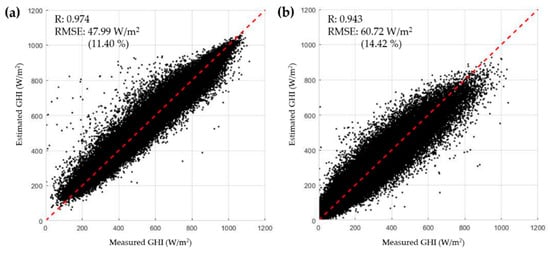
Figure 11.
Scatter plots of measured GHI and estimated GHI for (a) a clear sky, (b) a cloudy sky.
6.2. Solar Irradiance Map
Finally, hourly solar irradiance maps in Korea were generated from COMS images and the ANN ensemble model. Figure 12 shows an example of a generated hourly GHI map and COMS channel images at 14:00 on 1 January 2017 (KST). In Figure 12a, the northwest regions show lower GHI values compared to other regions, while southern regions show higher GHI. From Figure 12b–e, some clouds can be detected in the northwest. Clouds show higher values in the VIS and SWIR channels and lower values in the IR1 and IR2 channels than grounds [47]. It was found that the clouds had a significant impact on solar irradiance, mainly reducing it [48]. In addition, although the WV channel did not show a clear trend with solar irradiance in Figure 12f, this channel had a considerable impact on the solar irradiance because the model accuracy became reduced when training was conducted without the WV channel. Actually, water vapor is generally known to influence solar irradiance on the ground, especially in cloudless conditions [49].
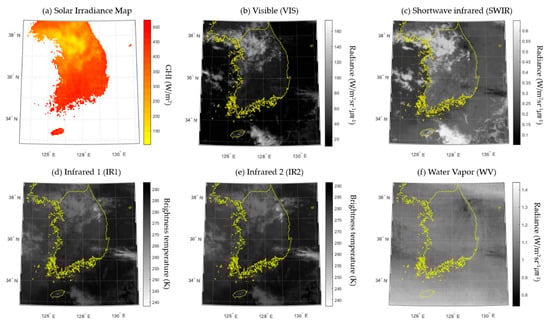
Figure 12.
Generated solar irradiance map and five input COMS images at 14:00 1 January 2017 (KST).
Figure 13 shows annual solar irradiance maps for Korea, for 2016 and 2017. The average solar irradiance was 3654 and 3874 Wh/m²/day for 2016 and 2017, respectively. The spatial distribution of GHI was slightly different between the two years, being higher in the northern region in 2016 but higher in the southeast region in 2017. In both years, relatively low solar irradiance was observed for Jeju Island in the south, and higher irradiance was noted for the western and southern small islands.
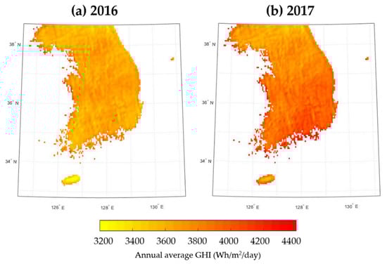
Figure 13.
Generated annual solar irradiance map using ANN models.
The annual GHI differences between results calculated using satellite data and ground measurement data, for 25 stations, are illustrated in Figure 14. A negative difference means that the GHI map estimation < measurement (underestimation), but a positive difference means that estimation > measurement (overestimation). In the northern stations (6, 7, 17), the GHI map shows that GHI was overestimated in both 2016 and 2017, and an overestimation trend was also shown for the southwest island stations (13, 19). In contrast, the GHI map shows that GHI was underestimated at some southwestern stations (3, 8, 10, 14, 22).
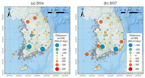
Figure 14.
Difference between satellite-derived and ground-derived annual GHI.
6.3. Significance and Limitations
The ANN model developed in this study showed better accuracy—an RMSE of 54.44 W/m² (12.93%)—than any other solar irradiance models applied to Korea. This model could estimate solar irradiance more accurately in clear sky than cloudy sky, with an RMSE value which was lower by approximately 13 W/m². In particular, by using COMS satellite data, this model could improve the estimation accuracy in cloudy skies compared to the previous MTSAT-based ANN method [30]. Since the temporal and spatial applicability of the ANN model for solar irradiance mapping were verified before developing the final ANN model, the solar irradiance maps could be produced by this ANN model and COMS satellite images. Considering the validation results, this model is expected to estimate hourly solar irradiance with an error level of <15%. Since COMS images cover all Korean territory every 15 min, GHI maps for Korea with a 4 km spatial resolution can be acquired every 15 min. This COMS-based ANN model can estimate solar irradiance over Korea, even where solar irradiance has not been measured, with better accuracy than the previous other data sources or methods. Therefore, by estimating solar irradiance for the entire country of Korea, this model can be used for the optimal site selection of solar PV systems and maximization of their efficiency by considering solar resources in Korea.
However, it is also important to be aware of some limitations of this model: first, using nearby satellite pixels can render some errors for solar irradiance estimations in coastal areas or islands. The radiance characteristics of land and sea water are different, as seen in Figure 12. Generally, compared to land, seawater shows lower radiance in the VIS and SWIR channels due to its low reflectance, and less variable brightness temperatures in the IR channels due to its high specific heat capacity. Since most of the GHI stations used in this study are inland, the resultant ANN model is not likely to reflect the radiation characteristics of the coastal or island areas whose neighboring pixels contain both land and sea. Actually, as shown in Figure 13, coastal areas and islands show relatively high GHI values compared to inland areas, and these values should be considered erroneous based on this limitation.
In addition, this satellite-based ANN model has difficulty estimating solar irradiance at smaller scales. The spatial resolution of this model is 4 km, which means that it cannot detect solar irradiance changes at scales <4 km. As an example of how this can occur, topography can cause either increased or reduced solar irradiance values for specific sites [50]. Since this model does not consider elevation or topographic effects, detailed shading or scattering effects caused by geographic characteristics cannot be reflected.
Finally, although it was proved that using the ANN method and a COMS satellite data source can improve the accuracy of solar irradiance estimation in Korea, the ANN used in this study has a relatively simple construction. Based on the potential of this simple ANN model for solar irradiance mapping in Korea, more sophisticated neural network techniques can be attempted for the further improvement of accuracy. For example, a convolutional neural network (CNN) has a possibility of improving the accuracy by adding a convolution layer of input satellite images and making the network deeper. In addition, a recurrent neural network (RNN) can have advantages in terms of the prediction of solar irradiance by using feedback connections.
7. Conclusions
In this study, hourly solar irradiance maps over Korea were generated by using an ensemble ANN model and COMS MI satellite images. Before developing the ANN model for solar irradiance mapping, ANN parameters were determined: the window size of the input satellite images (WS), the number of hidden layers (NL), and the number of nodes in each hidden layer (NN). After these parameters were determined, temporal and spatial applicability of ANN method for solar irradiance mapping were validated. The temporal generality of ANN method was evaluated by training the ANN model with 2016 data and testing it with 2017 data. Spatial generality was also evaluated by training the ANN model with the data from 19 train stations and testing it with the data from six test stations.
From the temporal and spatial validation, we concluded that the ANN method can be used for solar irradiance mapping in Korea, with significant accuracy. Therefore, based on these validation results, the final ANN ensemble model was developed from 10 independent ANN models. This model showed an R of 0.975 and RMSE of 54.44 W/m² (rRMSE 12.93%), which is more accurate than other previous works for Korea. This model exhibited no overfitting patterns between the train and test sets, and better accuracy in clear skies than cloudy skies. By using ANN as a solar irradiance derivation method and COMS MI images as data sources, it was proved that this approach can improve the accuracy of solar irradiance estimation for Korea.
The ANN model was then used to generate hourly GHI maps of Korea by using COMS images. The COMS-based ANN model developed in this study is expected to estimate real-time solar irradiance throughout Korea with significant accuracy (<15% error). Although there are some limitations of this model, and further works are needed to maximize its performance, it is meaningful that we found the possibility of using ANN and COMS data for accurate solar irradiance mapping. This model can contribute to assessing Korean solar resources and improving the efficiency of solar PV systems in Korea.
Author Contributions
Y.K. collected data, conducted ANN model training, testing, and validation, and wrote the first draft of this paper. M.O. built the ANN models and tested them for optimization, and established the irradiance map using the model. S.-M.K. revised the paper and advised on study systematization. H.-D.P. supervised the research and provided the research direction and sources. All authors have read and agreed to the published version of the manuscript.
Funding
This research was funded by the National Research Foundation of Korea (NRF) (No. NRF-2017R1A2B4007623).
Acknowledgments
This research was supported by the Brain Korea 21 Project.
Conflicts of Interest
The authors declare no conflict of interest.
References
- Kim, S.-M.; Oh, M.; Park, H.-D. Analysis and Prioritization of the Floating Photovoltaic System Potential for Reservoirs in Korea. Appl. Sci. 2019, 9, 395. [Google Scholar] [CrossRef]
- Şen, Z.; Şahin, A.D. Spatial interpolation and estimation of solar irradiation by cumulative semivariograms. Sol. Energy 2001, 71, 11–21. [Google Scholar] [CrossRef]
- Bezzi, M.; Vitti, A. A comparison of some kriging interpolation methods for the production of solar radiation maps. Geomat. Work 2005, 5, 1–17. [Google Scholar]
- Palmer, D.; Cole, I.; Betts, T.; Gottschalg, R. Interpolating and estimating horizontal diffuse solar irradiation to provide UK-wide coverage: Selection of the best performing models. Energies 2017, 10, 181. [Google Scholar] [CrossRef]
- Jamaly, M.; Kleissl, J. Spatiotemporal interpolation and forecast of irradiance data using Kriging. Sol. Energy 2017, 158, 407–423. [Google Scholar] [CrossRef]
- Yang, D.; Gu, C.; Dong, Z.; Jirutitijaroen, P.; Chen, N.; Walsh, W.M. Solar irradiance forecasting using spatial-temporal covariance structures and time-forward kriging. Renew. Energy 2013, 60, 235–245. [Google Scholar] [CrossRef]
- Journée, M.; Bertrand, C. Improving the spatio-temporal distribution of surface solar radiation data by merging ground and satellite measurements. Remote Sens. Environ. 2010, 114, 2692–2704. [Google Scholar] [CrossRef]
- Dev, S.; Sanoy, F.M.; Lee, Y.H.; Winkler, S. Estimating solar irradiance using sky imagers. Atmos. Meas. Tech. 2019, 12, 5417–5429. [Google Scholar] [CrossRef]
- Alonso-Montesinos, J.; Batlles, F.J. The use of a sky camera for solar radiation estimation based on digital image processing. Energy 2015, 90, 377–386. [Google Scholar] [CrossRef]
- Alonso-Montesinos, J.; Batlles, F.J.; Portillo, C. Solar irradiance forecasting at one-minute intervals for different sky conditions using sky camera images. Energy Convers. Manag. 2015, 105, 1166–1177. [Google Scholar] [CrossRef]
- Noia, M.; Ratto, C.F.; Festa, R. Solar Irradiance Estimation From Geostationary Satellite Data: 1. Statistical Models. Sol. Energy 1993, 51, 449–456. [Google Scholar] [CrossRef]
- Noia, M.; Ratto, C.F.; Festa, R. Solar Irradiance Estimation From Geostationary Satellite Data: 2. Physical Models. Sol. Energy 1993, 51, 457–465. [Google Scholar] [CrossRef]
- Perez, R.; Ineichen, P.; Moore, K.; Kmiecik, M.; Chain, C.; George, R.A.Y.; Vignola, F. A New Operational Model for Satellite-derived Irradiances: Description and Validation. Sol. Energy 2002, 73, 307–317. [Google Scholar] [CrossRef]
- Rigollier, C.; Lef, M.; Wald, L. The method Heliosat-2 for deriving shortwave solar radiation from satellite images. Sol. Energy 2004, 77, 159–169. [Google Scholar] [CrossRef]
- Choi, W.S.; Song, A.R.; Kim, Y. Il Solar Irradiance Estimation in Korea by Using Modified Heliosat-II Method and COMS-MI Imagery. J. Korean Soc. Surv. Geod. Photogramm. Cartogr. 2016, 33, 463–472. [Google Scholar]
- Linares-Rodriguez, A.; Ruiz-Arias, J.A.; Pozo-Vazquez, D.; Tovar-Pescador, J. An artificial neural network ensemble model for estimating global solar radiation from Meteosat satellite images. Energy 2013, 61, 636–645. [Google Scholar] [CrossRef]
- Gardner, M.W.; Dorling, S.R. Artificial neural networks (the multilayer perceptron)-a review of applications in the atmospheric sciences. Atmos. Environ. 1998, 32, 2627–2636. [Google Scholar] [CrossRef]
- Eissa, Y.; Marpu, P.R.; Gherboudj, I.; Ghedira, H.; Ouarda, T.B.M.J.; Chiesa, M. Artificial neural network based model for retrieval of the direct normal, diffuse horizontal and global horizontal irradiances using SEVIRI images. Sol. Energy 2013, 89, 1–16. [Google Scholar] [CrossRef]
- Alobaidi, M.H.; Marpu, P.R.; Ouarda, T.B.M.J.; Ghedira, H. Mapping of the solar irradiance in the UAE using advanced artificial neural network ensemble. IEEE J. Sel. Top. Appl. Earth Obs. Remote Sens. 2014, 7, 3668–3680. [Google Scholar] [CrossRef]
- Quesada-Ruiz, S.; Linares-Rodríguez, A.; Ruiz-Arias, J.A.; Pozo-Vazquez, D.; Tovar-Pescador, J. ScienceDirect An advanced ANN-based method to estimate hourly solar radiation from multi-spectral MSG imagery. Sol. Energy 2015, 115, 494–504. [Google Scholar] [CrossRef]
- Ameen, B.; Balzter, H.; Jarvis, C.; Wheeler, J. Modelling Hourly Global Horizontal Irradiance from Satellite-Derived Datasets and Climate Variables as New Inputs with Artificial Neural Networks. Energies 2019, 12, 148. [Google Scholar] [CrossRef]
- Marquez, R.; Pedro, H.T.C.; Coimbra, C.F.M. Hybrid solar forecasting method uses satellite imaging and ground telemetry as inputs to ANNs. Sol. Energy 2013, 92, 176–188. [Google Scholar] [CrossRef]
- Yeom, J.; Han, K.; Kim, J. Evaluation on Penetration Rate of Cloud for Incoming Solar Radiation Using Geostationary Satellite Data. Asia Pac. J. Atmos. Sci. 2012, 48, 115–123. [Google Scholar] [CrossRef]
- Kawamura, H.; Tanahashi, S.; Takahashi, T. Estimation of insolation over the Pacific Ocean off the Sanriku Coast. J. Oceanogr. 1998, 54, 457–464. [Google Scholar] [CrossRef]
- Zo, I.; Jee, J.; Lee, K. Development of GWNU ( Gangneung-Wonju National University ) One-Layer Transfer Model for Calculation of Solar Radiation Distribution of the Korean Peninsula. Asia Pac. J. Atmos. Sci. 2014, 50, 23–32. [Google Scholar] [CrossRef]
- Zo, I.; Jee, J.; Lee, K.; Kim, B. Analysis of Solar Radiation on the Surface Estimated from GWNU Solar Radiation Model with Temporal Resolution of Satellite Cloud Fraction. Asia Pac. J. Atmos. Sci. 2016, 52, 405–412. [Google Scholar] [CrossRef]
- Yeom, J.; Seo, Y.; Kim, D.; Han, K. Solar Radiation Received by Slopes Using COMS Imagery, a Physically Based Radiation Model, and GLOBE. J. Sens. 2016, 2016, 1–15. [Google Scholar] [CrossRef]
- Kim, C.K.; Kim, H.-G.; Kang, Y.-H.; Yun, C.-Y.; Lee, S.-N. Evaluation of Global Horizontal Irradiance Derived from CLAVR-x Model and COMS Imagery Over the Korean Peninsula. New Renew. Energy 2016, 12, 13–20. [Google Scholar] [CrossRef]
- Kim, C.K.; Kim, H.G.; Kang, Y.H.; Yun, C.Y. Toward Improved Solar Irradiance Forecasts: Comparison of the Global Horizontal Irradiances Derived from the COMS Satellite Imagery Over the Korean Peninsula. Pure Appl. Geophys. 2017, 174, 2773–2792. [Google Scholar] [CrossRef]
- Yeom, J.; Han, K. Computers & Geosciences Improved estimation of surface solar insolation using a neural network and MTSAT-1R data. Comput. Geosci. 2010, 36, 590–597. [Google Scholar]
- Famili, A.; Shen, W.-M.; Weber, R.; Simoudis, E. Data Preprocessing and Intelligent Data Analysis. Intell. Data Anal. 1997, 1, 3–23. [Google Scholar] [CrossRef]
- Hammer, A.; Heinemann, D.; Hoyer, C.; Kuhlemann, R.; Lorenz, E.; Müller, R.; Beyer, H.G. Solar energy assessment using remote sensing technologies. Remote Sens. Environ. 2003, 86, 423–432. [Google Scholar] [CrossRef]
- Eissa, Y.; Chiesa, M.; Ghedira, H. Assessment and recalibration of the Heliosat-2 method in global horizontal irradiance modeling over the desert environment of the UAE. Sol. Energy 2012, 86, 1816–1825. [Google Scholar] [CrossRef]
- Kuzniar, K.; Zajac, M. Some methods of pre-processing input data for neural networks. Comput. Assist. Methods Eng. Sci. 2015, 22, 141–151. [Google Scholar]
- Duffie, J.A.; Beckman, W.A. Solar Engineering of Thermal Processes, 3rd ed.; John Wiley & Sons, Inc.: Hoboken, NJ, USA, 2006; ISBN 0470873663. [Google Scholar]
- Marquez, R.; Coimbra, C.F.M. Forecasting of global and direct solar irradiance using stochastic learning methods, ground experiments and the NWS database. Sol. Energy 2011, 85, 746–756. [Google Scholar] [CrossRef]
- Haykin, S. Neural Networks and Learning Machines, 3rd ed.; Pearson Education, Inc.: Hoboken, NJ, USA, 2008; ISBN 9780131471399. [Google Scholar]
- Yousif, J.H.; Kazem, H.A.; Alattar, N.N.; Elhassan, I.I. A comparison study based on artificial neural network for assessing PV/T solar energy production. Case Stud. Therm. Eng. 2019, 13, 1–13. [Google Scholar] [CrossRef]
- Elsheikh, A.H.; Sharshir, S.W.; Elaziz, M.A.; Kabeel, A.E.; Guilan, W.; Haiou, Z. Modeling of solar energy systems using artificial neural network: A comprehensive review. Sol. Energy 2019, 180, 622–639. [Google Scholar] [CrossRef]
- Hagan, M.T.; Demuth, H.B.; Beale, M.H. Neural Network Design; PWS Publishing: Boston, MA, USA, 1996. [Google Scholar]
- Wang, F.; Mi, Z.; Su, S.; Zhao, H. Short-Term Solar Irradiance Forecasting Model Based on Artificial Neural Network Using Statistical Feature Parameters. Energies 2012, 5, 1355–1370. [Google Scholar] [CrossRef]
- Linares-Rodríguez, A.; Ruiz-Arias, J.A.; Pozo-Vázquez, D.; Tovar-Pescador, J. Generation of synthetic daily global solar radiation data based on ERA-Interim reanalysis and artificial neural networks. Energy 2011, 36, 5356–5365. [Google Scholar] [CrossRef]
- Nait Mensour, O.; Bouaddi, S.; Abnay, B.; Hlimi, B.; Ihlal, A. Mapping and Estimation of Monthly Global Solar Irradiation in Different Zones in Souss-Massa Area, Morocco, Using Artificial Neural Networks. Int. J. Photoenergy 2017, 2017, 1–19. [Google Scholar] [CrossRef]
- Mas, J.F.; Flores, J.J. The application of artificial neural networks to the analysis of remotely sensed data. Int. J. Remote Sens. 2008, 29, 617–663. [Google Scholar] [CrossRef]
- Stathakis, D. How many hidden layers and nodes? Int. J. Remote Sens. 2009, 30, 2133–2147. [Google Scholar] [CrossRef]
- Warren, S.G. Optical Properties of Snow. Rev. Geophys. 1982, 20, 67–89. [Google Scholar] [CrossRef]
- Rossow, W.B.; Garder, L.C. Cloud Detection Using Satellite Measurements of Infrared and Visible Radiances for ISCCP. J. Clim. 1993, 6, 2341–2369. [Google Scholar] [CrossRef]
- Xia, S.; Mestas-Nuñez, A.M.; Xie, H.; Vega, R. Satellite-based cloudiness and solar energy potential in Texas and surrounding regions. Remote Sens. 2019, 11, 1130. [Google Scholar] [CrossRef]
- López, G.; Gueymard, C.A.; Bosch, J.L.; Rapp-Arrarás, I.; Joaquín, A.-M.; Pulido-Calvo, I.; Ballestrín, J.; Polo, J.; Barbero, J. Modeling water vapor impacts on the solar irradiance reaching the receiver of a solar tower plant by means of artificial neural networks. Sol. Energy 2018, 169, 34–39. [Google Scholar] [CrossRef]
- Oh, M.; Park, H. A new algorithm using a pyramid dataset for calculating shadowing in solar potential mapping. Renew. Energy 2018, 126, 465–474. [Google Scholar] [CrossRef]


© 2020 by the authors. Licensee MDPI, Basel, Switzerland. This article is an open access article distributed under the terms and conditions of the Creative Commons Attribution (CC BY) license (http://creativecommons.org/licenses/by/4.0/).