A Linear Relaxation-Based Heuristic for Iron Ore Stockyard Energy Planning

 ,
,  and
and
Abstract
:1. Introduction
Contribution
2. Literature Review
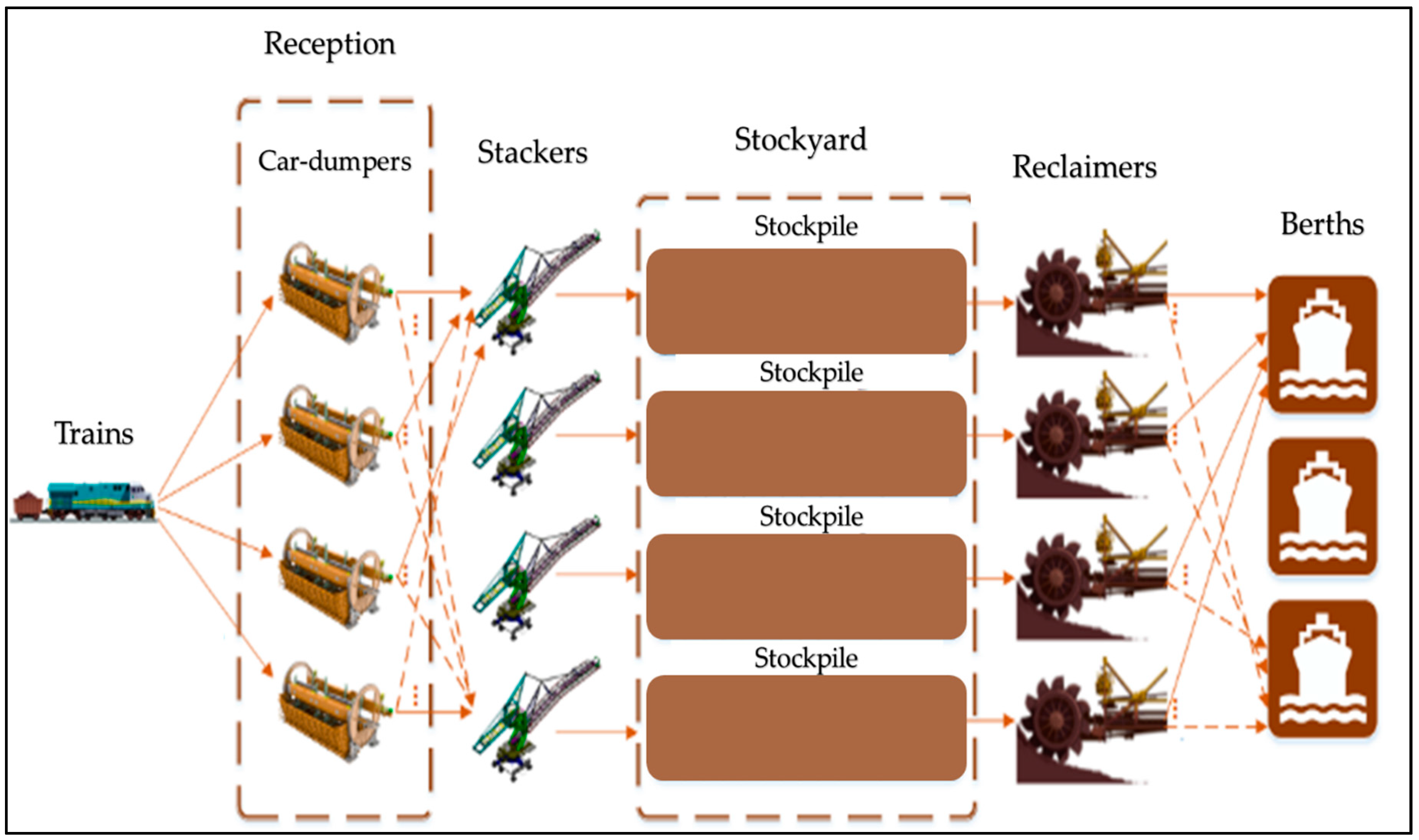
3. Problem Description
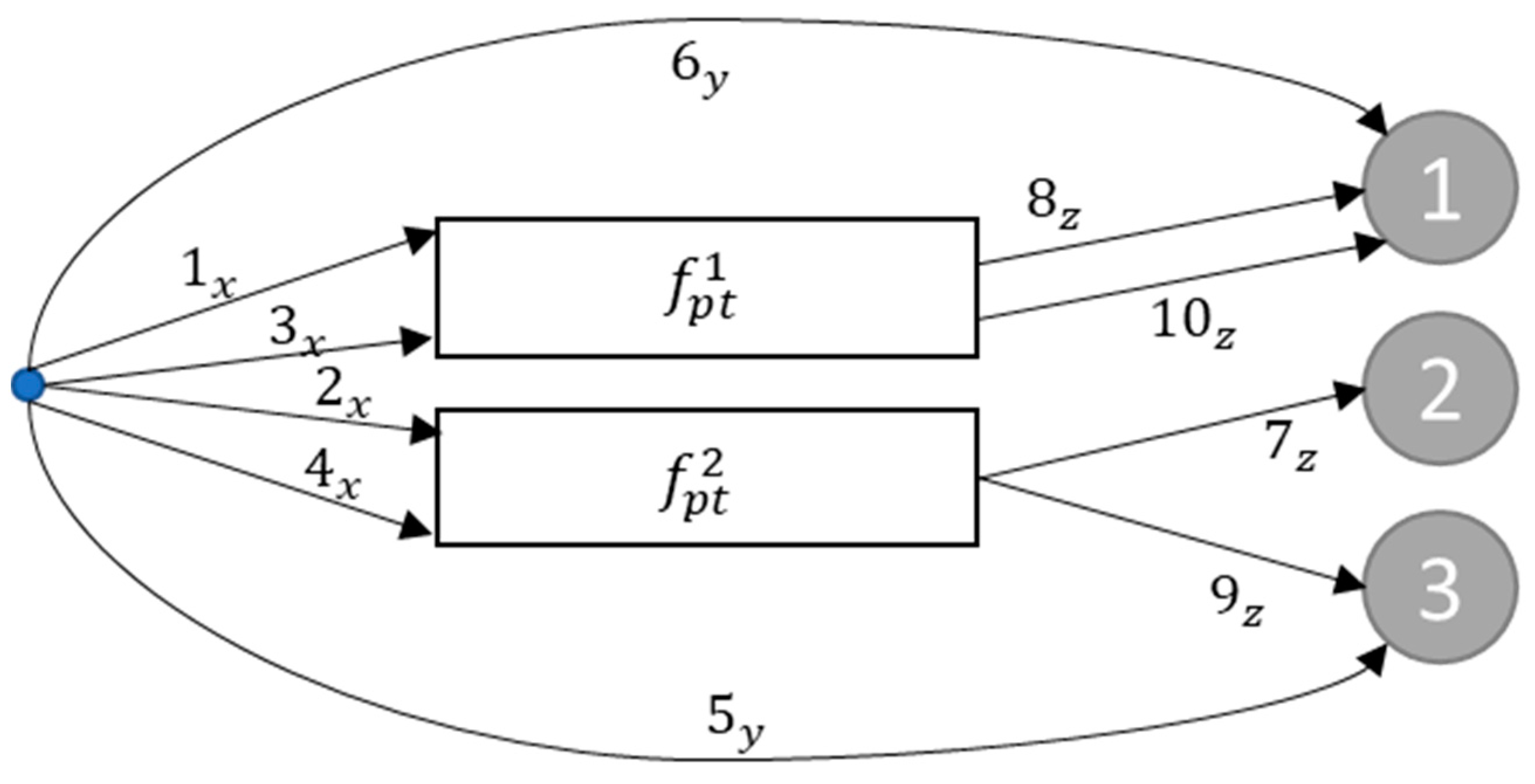
3.1. Problem Formulation
| Sets | |
| Set of periods; | |
| Set of products; | |
| Set of equipment; | |
| Set of storage sub-areas; | |
| Set of available mooring berths; | |
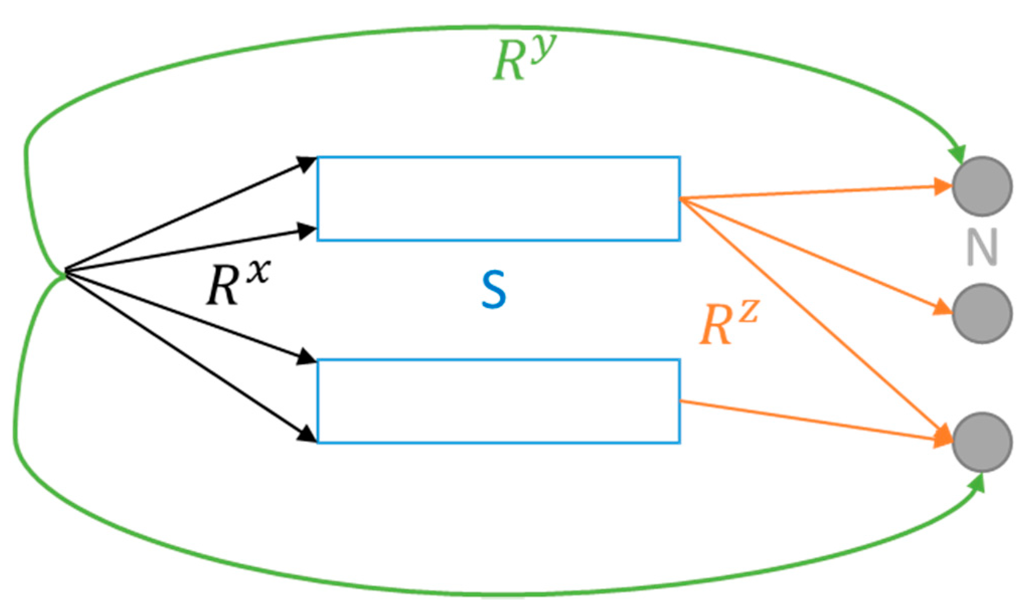
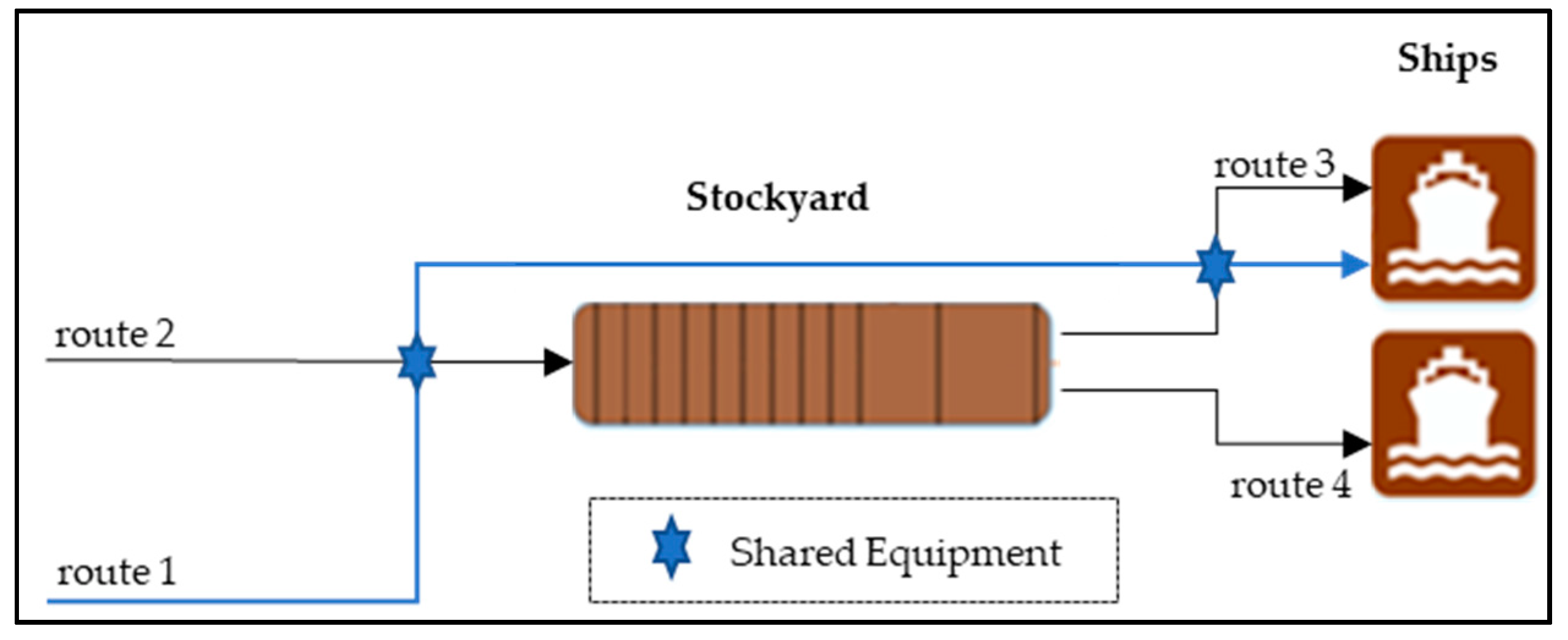
| Set of routes; | |
| Set of routes (receptions / stockyards); | |
| Set of routes (receptions / piers); | |
| Set of routes (stockyards / piers); | |
| Subset of routes that reach subarea ; | |
| Subset of routes that from subarea ; | |
| Subset of routes that reach pier ; | |
| Subset of routes that reach pier ; | |
| Subset of routes that use equipment ; | |
| Subset of routes that use equipment ; | |
| Subset of routes that use equipment . | |
| Parameters | |
| Energy cost to use the route in period ; | |
| Energy cost to keep in the product in storage sub-area during period ; | |
| Energy cost for not meeting the supply and keeping product at the reception in period ; | |
| Capacity (in tons/hour) of route ; | |
| Capacity (in tons/hour) of route ; | |
| Capacity (in tons/hour) of route ; | |
| Energy cost associated with replacing product with product to meet the demand of product ; | |
| Available time (in hours) for the use of equipment in period ; | |
| Capacity of equipment (in tons/hour); | |
| Supply of product at the beginning of period ; | |
| Demand of product for a ship moored at berth at the beginning of period | |
| Storage capacity of subarea for product p in period . | |
| Time taken in period t to transport product from the reception to the stockyard using route . | |
| Time taken to transport product to meet the demand of product in period using route . When is equal to , the product delivered is the same as what was requested. | |
| Time taken to transport product to meet the demand of product in period using route . When is equal to , the product delivered is the same as what was requested. | |
| Represents the amount of product in the reception subsystem that was not delivered at the end of period . | |
| Amount of product stored in subarea during period . | |
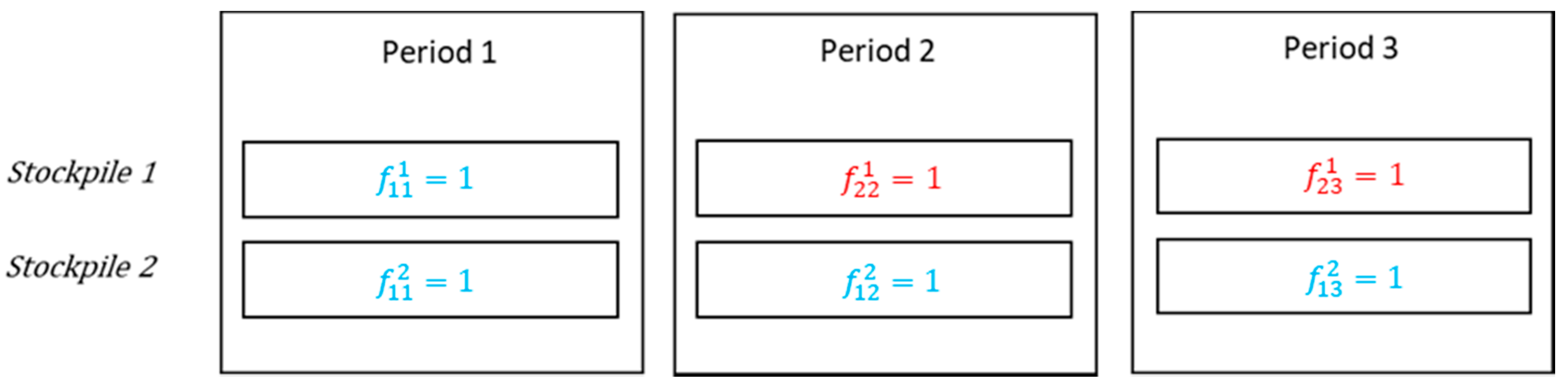
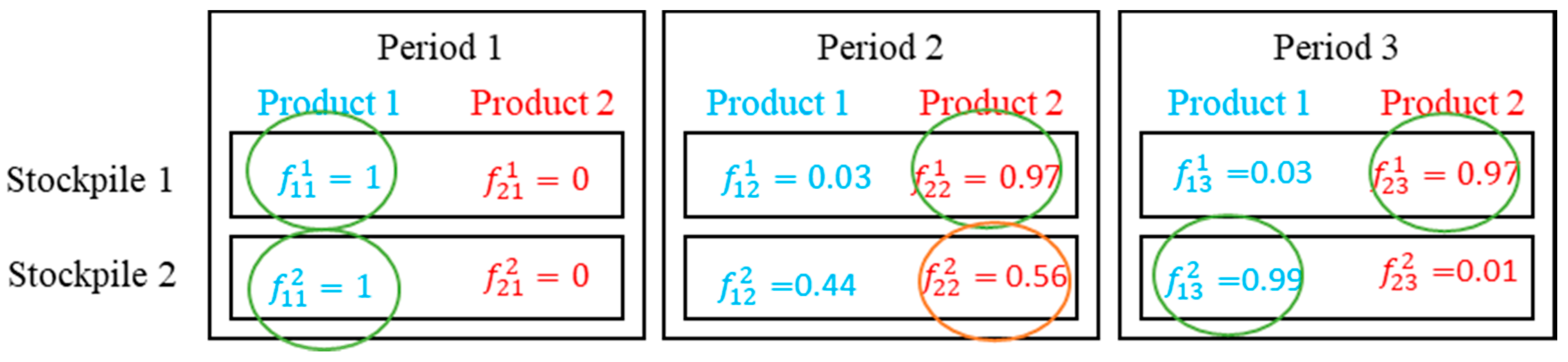
| when subarea is allocated to product in period ; otherwise. | |
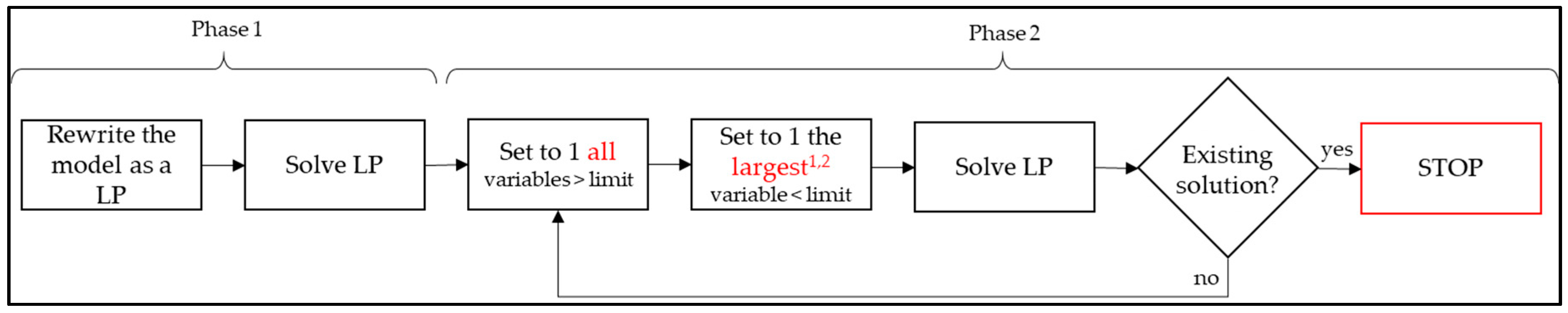
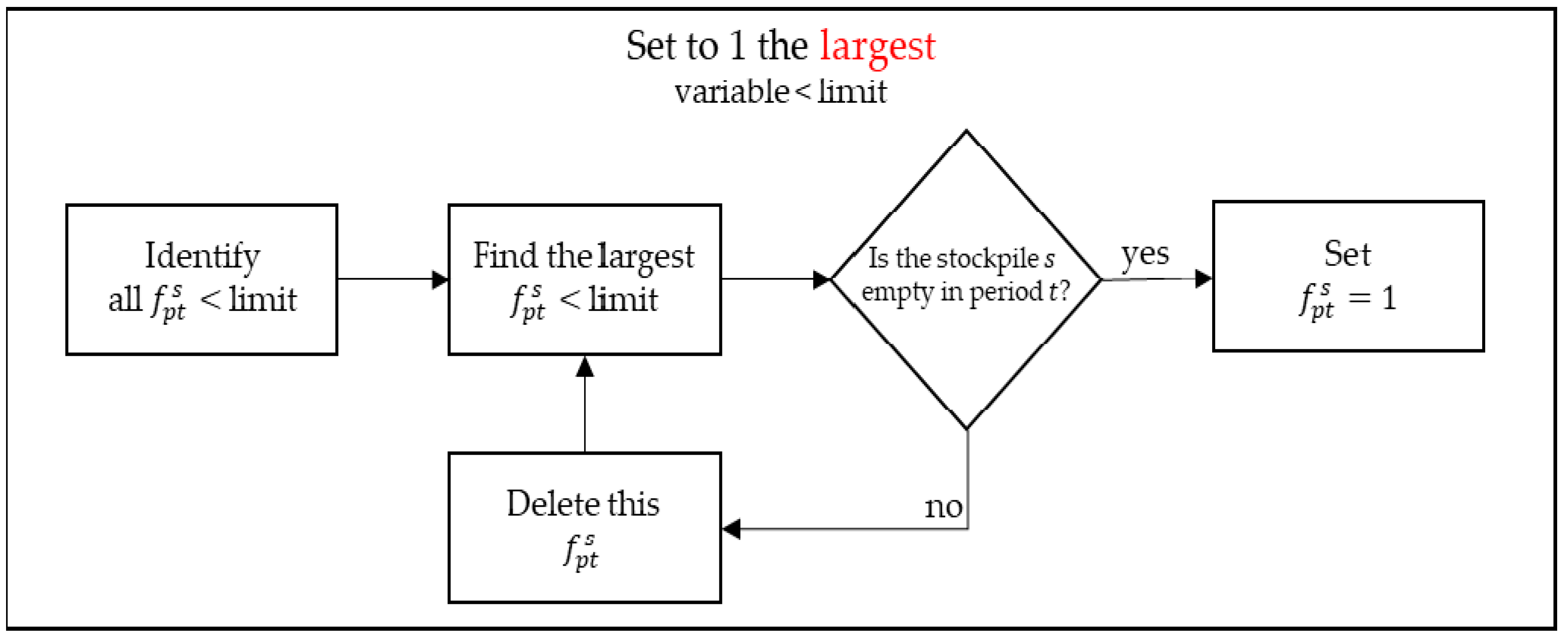
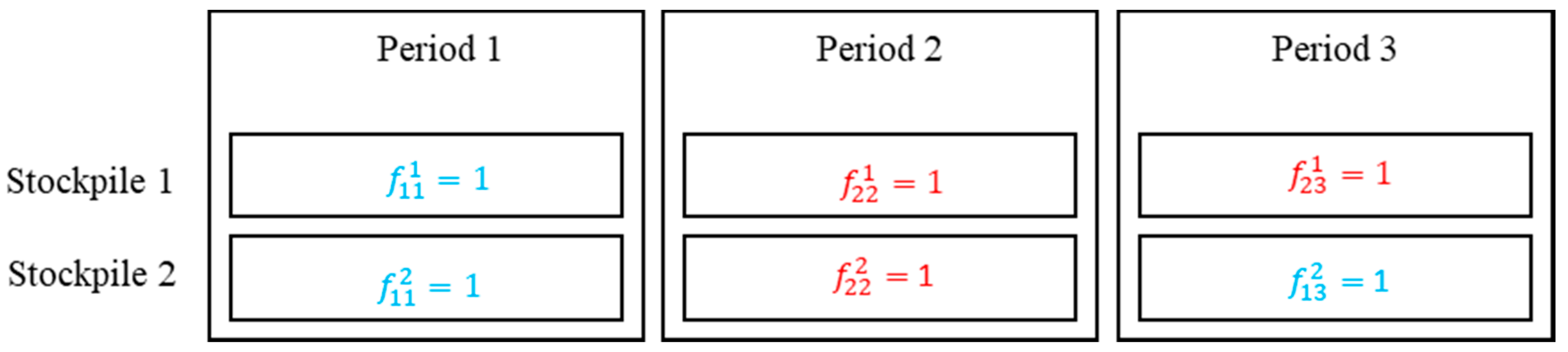
3.2. Linear Relaxation-Based Heuristic
| Algorithm 1. Setting binaries variables for stacking a stockpile. |
| Rewrite the model Solve (LP) while there are some or do if limit do end if for largest empty stockpile limit do end for Rewrite the model with set variables. Solve (LP) end while |
4. Computational Tests and Discussion
4.1. Physical Characteristics of the Iron Ore Stockyard Proposal
4.2. Computational Results
5. Conclusions
Author Contributions
Funding
Acknowledgments
Conflicts of Interest
References
- Servare Junior, M.W.J.; Cardoso, P.A.; Cruz, M.M.C.; Paiva, M.H.M. Mathematical model for supply chain design with time postponement. Transportes 2018, 26, 1–15. [Google Scholar] [CrossRef] [Green Version]
- Floudas, C.A.; Lin, X. Continuous-time versus discrete-time approaches for scheduling of chemical processes: A review. Comput. Chem. Eng. 2004, 28, 2109–2129. [Google Scholar] [CrossRef] [Green Version]
- Méndez, C.A.; Cerdá, J.; Grossmann, I.E.; Harjunkoski, I.; Fahl, M. State-of-the-art review of optimization methods for short-term scheduling of batch processes. Comput. Chem. Eng. 2006, 30, 913–946. [Google Scholar] [CrossRef] [Green Version]
- Li, Z.; Ierapetritou, M. Process scheduling under uncertainty: Review and challenges. Comput. Chem. Eng. 2008, 32, 715–727. [Google Scholar] [CrossRef]
- Li, Z.; Ierapetritou, M.G. Robust optimization for process scheduling under uncertainty. Ind. Eng. Chem. Res. 2008, 47, 4148–4157. [Google Scholar] [CrossRef]
- Ribas, I.; Leisten, R.; Framiñan, J.M. Review and classification of hybrid flow shop scheduling problems from a production system and a solutions procedure perspective. Comput. Oper. Res. 2010, 37, 1439–1454. [Google Scholar] [CrossRef]
- Phanden, R.K.; Jain, A.; Verma, R. Integration of process planning and scheduling: A state-of-the-art review. Int. J. Comput. Integr. Manuf. 2011, 24, 517–534. [Google Scholar] [CrossRef]
- Maravelias, C.T. General framework and modeling approach classification for chemical production scheduling. AIChE J. 2012, 58, 1812–1828. [Google Scholar] [CrossRef]
- Servare Junior, M.W.J.; Rocha, H.R.O.; Salles, J.L.F. A multi-product mathematical model for iron ore stockyard planning problem. Braz. J. Dev. 2020, 6, 45076–45089. [Google Scholar] [CrossRef]
- CPLEX. IBM ILOG. V12. 1: User’s Manual for CPLEX; International Business Machines Corporation: Armonk, NY, USA, 2009; Volume 46, p. 157. [Google Scholar]
- Voudoris, C. Guided Local Search for Combinatorial Optimization Problems. Ph.D. Thesis, University of Essex, Colchester, UK, 1997. [Google Scholar]
- Abdekhodaee, A.; Dunstall, S.; Ernst, A.T.; Lam, L. Integration of stockyard and rail network: A scheduling case study. In Proceedings of the 5th Asia-Pacific Industrial Engineering and Management Systems Conference, Gold Coast, Australia, 12–15 December 2004; pp. 1–16. [Google Scholar]
- Boland, N.; Gulczynski, D.; Savelsbergh, M. A stockyard planning problem. EURO J. Transp. Logist. 2012, 1, 197–236. [Google Scholar] [CrossRef] [Green Version]
- Lu, T.F. Modeling for stockpile operations associated with bulk solid materials using bucket wheel reclaimer. Int. J. Inf. Acquis. 2010, 7, 357–373. [Google Scholar] [CrossRef]
- Hu, D.; Yao, Z. Stacker-reclaimer scheduling in a dry bulk terminal. Int. J. Comput. Integr. Manuf. 2012, 25, 1047–1058. [Google Scholar] [CrossRef]
- Van Vianen, T.A.; Ottjes, J.A.; Negenborn, R.R.; Lodewijks, G.; Mooijman, D.L. Simulation-based operational control of a dry bulk terminal. In Proceedings of the 9th IEEE International Conference on Networking, Sensing and Control, Beijing, China, 11–14 April 2012; pp. 73–78. [Google Scholar] [CrossRef]
- Hanoun, S.; Khan, B.; Johnstone, M.; Nahavandi, S.; Creighton, D. An effective heuristic for stockyard planning and machinery scheduling at a coal handling facility. In Proceedings of the 11th IEEE International Conference on Industrial Informatics (INDIN), Bochum, Germany, 29–31 July 2013; pp. 206–211. [Google Scholar] [CrossRef]
- Boland, N.; Savelsbergh, M.; Waterer, H. Shipping data generation for the hunter valley coal chain. Optim. Online 2013, 2, 3755. [Google Scholar]
- Savelsbergh, M.; Kapoor, R. Optimizing Reclaimer Schedules. In Proceedings of the 22nd National Conference of the Australian Society for Operations Research, Adelaide, Australia, 1–6 December 2013; pp. 272–278. [Google Scholar]
- Van Vianen, T.; Ottjes, J.; Lodewijks, G. Simulation-based determination of the required stockyard size for dry bulk terminals. Simul. Model. Pract. Theory 2014, 42, 119–128. [Google Scholar] [CrossRef]
- Van Vianen, T.; Ottjes, J.; Lodewijks, G. Simulation-based rescheduling of the stacker–reclaimer operation. J. Comput. Sci. 2015, 10, 149–154. [Google Scholar] [CrossRef]
- Savelsbergh, M.; Smith, O. Cargo assembly planning. EURO J. Transp. Logist. 2015, 4, 321–354. [Google Scholar] [CrossRef]
- Kalinowski, T.; Kapoor, R.; Savelsbergh, M.W. Scheduling reclaimers serving a stock pad at a coal terminal. J. Sched. 2017, 20, 85–101. [Google Scholar] [CrossRef]
- Menezes, G.C.; Mateus, G.R.; Ravetti, M.G. A branch and price algorithm to solve the integrated production planning and scheduling in bulk ports. Eur. J. Oper. Res. 2017, 258, 926–937. [Google Scholar] [CrossRef]
- Dafnomilis, I.; Duinkerken, M.B.; Junginger, M.; Lodewijks, G.; Schott, D.L. Optimal equipment deployment for biomass terminal operations. Transp. Res. Part E Logist. Transp. Rev. 2018, 115, 147–163. [Google Scholar] [CrossRef]
- Unsal, O.; Oguz, C. An exact algorithm for integrated planning of operations in dry bulk terminals. Transp. Res. Part E Logist. Transp. Rev. 2019, 126, 103–121. [Google Scholar] [CrossRef]
- Thanh, P.N.; Péton, O.; Bostel, N. A linear relaxation-based heuristic approach for logistics network design. Comput. Ind. Eng. 2010, 59, 964–975. [Google Scholar] [CrossRef]

| Problem Definition | Objectives | ||
| SPr | Single Period | Age | Minimize average age of stockpile |
| Mpr | Multi-Period | Cost | Minimize the total cost |
| SP | Single Product | Del | Minimize the delay of planning |
| MP | Multi-Product | Dev | Minimize the deviation of planning |
| D | Deterministic | Etime | Minimize the sum of the reclaim end times |
| S | Stochastic | MS | Minimize the makespan |
| CF | Capacitated Flow | Pen | Minimize penalties for not meet the planning |
| UCF | Uncapacitated Flow | Ships | Maximize the amount of ships served |
| Ca | Capacitated Facility | Thro | Maximize the throughput |
| UCa | Uncapacitated Facility | Time | Minimize the end time of reclaimers |
| Modelling | Wait | Minimize the waiting time of cargo trains | |
| LP | Linear Programming | Solution Method | |
| MILP | Mixed Integer Linear Programming | CAP | Cargo Assembly Planning Algorithm |
| MINLP | Mixed Integer Non-Linear Programming | CG | Column Generation |
| MIP | Mixed Integer Programming | GA | Genetic Algorithm |
| SMIP | Stochastic Mixed Integer Programming | GH | Greedy Heuristic |
| Reference Papers | Problem Definition | Type of Stockyard | Modelling | Objectives | Solution Method |
|---|---|---|---|---|---|
| [12] | MPr, MP, D, CF, UCa | Coal | MIP | Pen | Exact and GH |
| [13] | SPr, MP, D, UCF, Ca | Coal | MILP | Del | Exact and GH |
| [14] | SPr, SP, S, CF, Ca | Solid Bulk | - | - | Simulation |
| [15] | SPr, SP, D, UCF, Ca | Iron Ore | MIP | MS | Exact and GA |
| [16] | SPr, SP, S, CF, Ca | Solid Bulk | - | - | Simulation |
| [17] | MPr, MP, D, UCF, Ca | Coal | LP | Del/Age | Exact and Heuristic |
| [18] | SPr, MP, D, UCF, UCa | Coal | MINLP | Dev | Exact |
| [19] | Mpr, MP, D. CF, Ca | Coal | - | Time | Approximation Algorithm |
| [20] | SPr, SP, S, CF, Ca | Solid Bulk | - | - | Simulation |
| [21] | SPr, SP, S, CF, Ca | Dry Bulk | - | Wait- | Simulation |
| [22] | MPr, SP, D. UCF, Ca | Coal | - | Thro | CAP |
| [23] | MPr, SP, D, UCF, UCa | Coal | MIP | Etime | Exact |
| [24] | MPr, MP, D, CF, Ca | Iron Ore | MILP | Costs | Exact and CG |
| [25] | SPr, SP, D, UCF, Ca | Biomass | MILP | Costs | Exact |
| [26] | MPr, SP, D, CF, Ca | Dry Bulk | MIP | Time | Exact |
| [9] | MPr, MP, D, CF, Ca | Iron Ore | MILP | Ships | Exact |
| Problem Definition | Type of Stockyard | Modelling | Objectives | Solution Method |
|---|---|---|---|---|
| MPr, MP, D, CF, Ca | Iron Ore | MILP | Energy | Exact and LBRH |
| Parameter | Range |
|---|---|
| Total demand | Uniform (3–4) |
| Berth capacity | Uniform (100–200) |
| Equipment capacity | Uniform (100–200) |
| Stockpile capacity | Uniform (1000–1800) |
| Car-dumper capacity | Uniform (40–60) |
| Supply capacity | Uniform (500–800) |
| Conveyor belt capacity | Uniform (80–120) |
| Amount of equipment by route | Uniform (2–4) |
| Available time | Uniform (2–5) |
| Energy cost by period | Uniform (1–3) |
| Cost of not transferring the ore from reception | Uniform (20–30) |
| Cost of keeping the ore in stockyard | Uniform (1–2) |
| Cost due to change in the quality of the ore | Uniform (10–20) |
| System Features | Amount |
|---|---|
| Stockyards | 2 |
| Berths | 3 |
| Routes | 10 |
| Routes X | 4 |
| Routes Z | 4 |
| Routes Y | 2 |
| Equipment in the system | 20 |
| Equipment in Routes X | 9 |
| Equipment in Routes Z | 6 |
| Equipment in Routes Y | 5 |
| Instance | Product Types | Planning Horizon (Periods) |
|---|---|---|
| 1 | 2 | 3 |
| 2 | 3 | 6 |
| 3 | 4 | 12 |
| 4 | 7 | 18 |
| 5 | 10 | 24 |
| 6 | 10 | 48 |
| 7 | 10 | 72 |
| 8 | 12 | 168 |
| 9 | 12 | 240 |
| 10 | 15 | 336 |
| 11 | 15 | 720 |
| 12 | 20 | 720 |
| 13 | 25 | 1440 |
| 14 | 30 | 1800 |
| 15 | 30 | 2160 |
| 16 | 30 | 2400 |
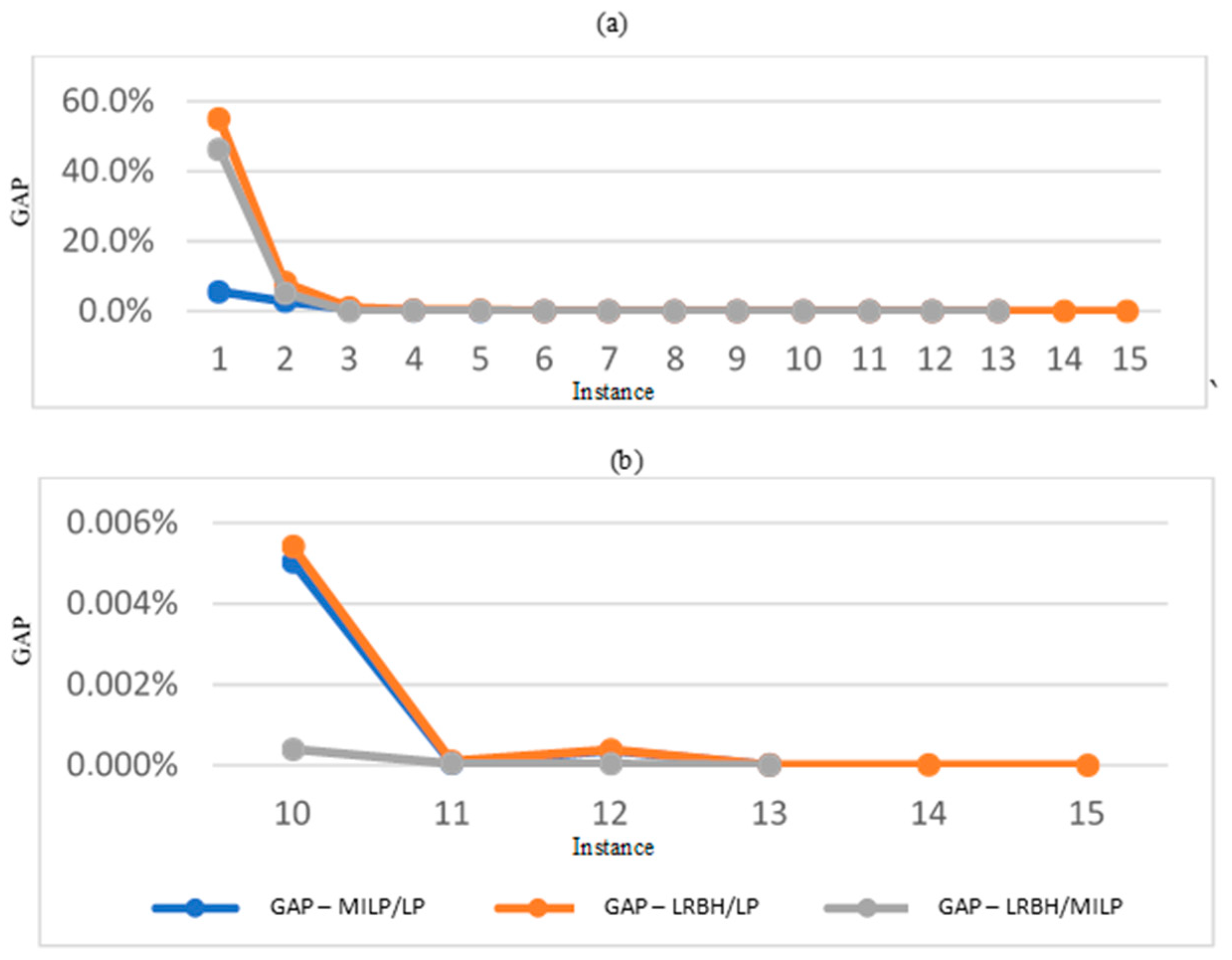
| Instance | TIME-MILP (s) | TIME-LP (s) | TIME-LRBH (s) | TOTAL TIME-LRBH (s) | GAP-LRBH /MILP (%) | Iterations |
|---|---|---|---|---|---|---|
| 1 | 0.000 | 0.000 | 0.015 | 0.015 | 46.292000 | 1 |
| 2 | 0.000 | 0.000 | 0.125 | 0.125 | 5.165446 | 4 |
| 3 | 0.047 | 0.032 | 0.172 | 0.204 | 0.039728 | 1 |
| 4 | 0.266 | 0.125 | 1.812 | 1.937 | 0.170065 | 4 |
| 5 | 1.469 | 0.359 | 5.251 | 5.61 | 0.217760 | 7 |
| 6 | 1.079 | 0.532 | 3.969 | 4.501 | 0.000983 | 3 |
| 7 | 1.172 | 0.907 | 7.14 | 8.047 | 0.003256 | 4 |
| 8 | 6.672 | 4.031 | 23.098 | 27.129 | 0.000000 | 2 |
| 9 | 9.407 | 5.734 | 21.785 | 27.519 | 0.000552 | 4 |
| 10 | 34.021 | 13.814 | 115.655 | 129.469 | 0.000396 | 5 |
| 11 | 145.24 | 32.54 | 114.401 | 146.941 | 0.000046 | 2 |
| 12 | 321.92 | 67.418 | 422.914 | 490.332 | 0.000030 | 4 |
| 13 | 5031.883 | 313.684 | 854.06 | 1167.744 | 0.000003 | 2 |
| 14 | 2 | 1127.522 | 3378.492 | 4506.014 | - | 3 |
| 15 | 2 | 1060.815 | 4249.165 | 5309.98 | - | 3 |
| 16 | 2 | - | - | 3 | - | - |
| Instance | GAP-MILP/LP (%) | GAP-LRBH/LP (%) |
|---|---|---|
| 1 | 5.622750 | 55.007652 |
| 2 | 2.819756 | 8.216897 |
| 3 | 0.634561 | 1.038426 |
| 4 | 0.190741 | 0.361495 |
| 5 | 0.107536 | 0.325647 |
| 6 | 0.030696 | 0.040535 |
| 7 | 0.007023 | 0.010280 |
| 8 | 0.001033 | 0.001033 |
| 9 | 0.000407 | 0.000959 |
| 10 | 0.005030 | 0.005426 |
| 11 | 0.000052 | 0.000098 |
| 12 | 0.000355 | 0.000385 |
| 13 | 0.000008 | 0.000011 |
| 14 | - | 0.000008 |
| 15 | - | 0.000004 |
© 2020 by the authors. Licensee MDPI, Basel, Switzerland. This article is an open access article distributed under the terms and conditions of the Creative Commons Attribution (CC BY) license (http://creativecommons.org/licenses/by/4.0/).
Share and Cite
Servare Junior, M.W.J.; Rocha, H.R.d.O.; Salles, J.L.F.; Perron, S. A Linear Relaxation-Based Heuristic for Iron Ore Stockyard Energy Planning. Energies 2020, 13, 5232. https://doi.org/10.3390/en13195232
Servare Junior MWJ, Rocha HRdO, Salles JLF, Perron S. A Linear Relaxation-Based Heuristic for Iron Ore Stockyard Energy Planning. Energies. 2020; 13(19):5232. https://doi.org/10.3390/en13195232
Chicago/Turabian StyleServare Junior, Marcos Wagner Jesus, Helder Roberto de Oliveira Rocha, José Leandro Félix Salles, and Sylvain Perron. 2020. "A Linear Relaxation-Based Heuristic for Iron Ore Stockyard Energy Planning" Energies 13, no. 19: 5232. https://doi.org/10.3390/en13195232
APA StyleServare Junior, M. W. J., Rocha, H. R. d. O., Salles, J. L. F., & Perron, S. (2020). A Linear Relaxation-Based Heuristic for Iron Ore Stockyard Energy Planning. Energies, 13(19), 5232. https://doi.org/10.3390/en13195232