Clarke Transformation Solution of Asymmetrical Transients in Three-Phase Circuits

Abstract

This work deals with the use of the Clarke transformation for the theoretical derivation of circuit models for the analysis of asymmetrical transients in three-phase circuits. Asymmetrical transients occur when only one or two phases of a three-phase power system are involved in a switch operation. Such a condition is critical from a theoretical viewpoint since the Clarke transformation is based on the assumption of circuit symmetry between the three phases. If the symmetry assumption is not met, the equivalent circuits in the transformed variables α, β, and 0 are not uncoupled. The literature concerning numerical approaches for asymmetrical transient analysis is very rich, but a comprehensive and rigorous analytical investigation of circuit models within the framework of the Clarke transformation is still lacking. Contrary to numerical approaches, analytical solutions provide deeper insight into the phenomenon and allow for theoretical interpretation and better understanding of the transient behavior. The proposed circuit models show that the β variables are always uncoupled with α and 0 variables, whereas coupling between α and 0 variables can be properly represented by an ideal transformer. Moreover, in the case of single-line switching, the β variables have no transient, i.e., they keep the steady-state behavior. Transient properties can be readily and effectively observed by representing the trajectory of the space vector on the complex plane. All the analytical results have been checked numerically through the Simulink (Matlab R2020a, The MathWorks, Inc., Natick, MA, USA) implementation of a specific three-phase circuit introduced to illustrate the main theoretical issues.

1. Introduction

Transformation methods for circuit analysis of three-phase power systems have a long and important history in electrical engineering. Symmetrical components and Clarke transformations are well-known examples of such mathematical tools [1,2]. From a modern perspective, three-phase transformation methods can be considered as special cases of a more general approach consisting of the decoupling of system equations through matrix diagonalization [3,4]. Decoupled equations can be easily solved provided that the transformed variables (i.e., the modal variables) are used instead of the natural variables. Finally, inverse transformation allows the evaluation of the solution in terms of natural variables. Identification of the transformation matrix which is able to diagonalize the system matrix is the crucial point of the methodology. In the most general case, such identification can be obtained numerically for each specific system to be solved [5]. When three-phase power systems come into play, however, system matrices (i.e., resistance, inductance, and capacitance matrices) show a specific symmetrical structure originating from the common assumption of circuit symmetry between the three phases. Such an assumption allows the analytical and a priori determination of the transformation matrices. The symmetrical components’ transformation operates on phasors, and the corresponding transformation matrix is complex. The Clarke transformation operates on time-domain variables, and the corresponding transformation matrix is real.

Transient analysis of three-phase circuits is a topic of paramount importance in modern power systems where a huge number of electronic and electromechanical components are scattered along the networks and are continuously connected and disconnected. The dynamic circuit elements included in such components produce overcurrents/voltages when the topology of the network is sharply changed by the operation of switches. Prediction and evaluation of overcurrents/voltages is important in order to prevent malfunctioning and damage of other components and subsystems [6,7,8,9]. As far as transient analysis of three-phase circuits is concerned, the Clarke transformation is the natural candidate since it operates in the time domain [10,11,12,13]. In fact, a general methodology for the analysis of three-phase symmetrical transients based on the Clarke transformation and the related concept of space vector has been recently published [14].

If asymmetrical transients are considered, however, the general methodology outlined above is invalidated [15,16,17]. In fact, asymmetrical transients originate from a switch operation of one or two phases in a specific section of a three-phase circuit. Such asymmetrical operation introduces circuit asymmetry between the three phases, and therefore the straightforward use of the Clarke transformation is prevented. The analysis of asymmetrical transients in terms of the Clarke transformation and the space vector concept, however, would be of great interest because of the widespread use of such mathematical tools.

The main objective of this work is the definition of a general methodology for the analytical solution of asymmetrical transients based on the Clarke transformation. Asymmetry between the three phases requires specific theoretical work since the straightforward application of the Clarke transformation does not produce diagonalization of system matrices. Analytical solutions in closed form are derived based on meaningful interpretation and representation of interaction between Clarke modal circuits (i.e., α, β, and 0 circuits) due to phase asymmetry.

The proposed analytical approach provides theoretical insight into the comprehension of asymmetrical transients by explaining the role of each Clarke modal circuit in the determination of the time-domain phase variables. A comparable analytical contribution is not available in the relevant literature, whereas the literature concerning the numerical simulation of transients in three-phase systems is vast (e.g., see [7,18,19,20,21,22]). In particular, time-domain and frequency-domain analysis of asymmetrical transients has proved to be effective in the characterization of faults in electrical machines, power lines, and power electronics systems [23,24,25,26,27,28,29,30,31,32]. Therefore, the analytical results derived in this paper can provide theoretical support to both existing and new methodologies for fault characterization.

This paper is organized as follows. In Section 2, the background concerning Clarke transformation and the space vector properties is recalled. In Section 3, the proposed methodology for Clarke circuit modeling of asymmetrical transients is derived in the Laplace domain. In particular, the two cases corresponding to single-line and two-line switching are treated separately and in detail. Frequency-domain analysis provides very simple results from a formal viewpoint, but inverse Laplace transform is needed to obtain explicit time-domain solutions. In Section 4, the proposed methodology is developed directly in the time domain. Explicit time-domain solutions are obtained through the conventional state-equation approach applied to α, β, and 0 circuits instead of the whole three-phase circuit. Analytical results are validated in Section 5 through the Simulink implementation of a specific three-phase circuit used to illustrate the main theoretical properties derived in Section 3 and Section 4. Finally, conclusions are drawn in Section 6.

2. Background: The Clarke Transformation

Since the objective of this work is the transient (i.e., time domain) analysis of three-phase circuits due to line switching, the most suitable mathematical tool is a transformation operating in the time domain, such as the Clarke transformation. In fact, the well-known symmetrical components transformation is not suited to the present objective since it is operating on phasor quantities (i.e., in the frequency domain). It will be shown that a proper (non-conventional) use of the Clarke transformation allows the derivation of closed-form analytical solutions for time-domain voltages and currents in three-phase circuits after instantaneous switching of one or two lines. Such a kind of circuit operation introduces asymmetry in a three-phase circuit (because only one or two lines are involved in the switching). For this reason, a non-conventional use of the Clarke transformation is required, since its conventional use assumes circuit symmetry of the three phases.

The Clarke transformation applies to each triplet of phase time-domain variables a, b, c (voltages or currents) in a given three-phase circuit. For example, by considering a triplet of phase currents (similar results hold for phase voltages):

$$\left[\begin{array}{c}{i}_{\alpha }\\ i_{\beta }\\ i_0\end{array}\right]=\mathit{T}\left[\begin{array}{c}{i}_a\\ i_b\\ i_c\end{array}\right]=\sqrt{\frac{2}{3}}\left[\begin{array}{ccc}1& -1/2& -1/2\\ 0& \sqrt{3}/2& -\sqrt{3}/2\\ 1/\sqrt{2}& 1/\sqrt{2}& 1/\sqrt{2}\end{array}\right]\left[\begin{array}{c}{i}_a\\ i_b\\ i_c\end{array}\right]$$

(1)

Notice that in Equation (1), the rational form of the Clarke transformation was used (i.e., the factor $\sqrt{2/3}$ was introduced). This choice corresponds to orthogonality of the transformation matrix T (i.e., ${\mathit{T}}^{-1}={\mathit{T}}^{\mathit{t}}$), leading to the conservation of power through the transformation.

Under the assumption of circuit symmetry of the three phases, a phase inductance matrix L (and capacitance/resistance matrices, if needed) is diagonalized by the Clarke matrix T:

$${\mathit{L}}_{\mathit{T}}=\mathit{T}\mathit{L}{\mathit{T}}^{-1}=\mathit{T}\left[\begin{array}{ccc}{L}_p& L_m& L_m\\ L_m& L_p& L_m\\ L_m& L_m& L_p\end{array}\right]{\mathit{T}}^{-1}=\left[\begin{array}{ccc}{L}_{\alpha }& 0& 0\\ 0& L_{\beta }& 0\\ 0& 0& L_0\end{array}\right]$$

(2)

where $L_{\alpha }=L_{\beta }=L_p-L_m$ and $L_0=L_p+2L_m$.

Thus, under the assumption of circuit symmetry, the use of the Clarke transformation for all the phase variables and all the three-phase components leads to three uncoupled modal circuits α, β, and 0. 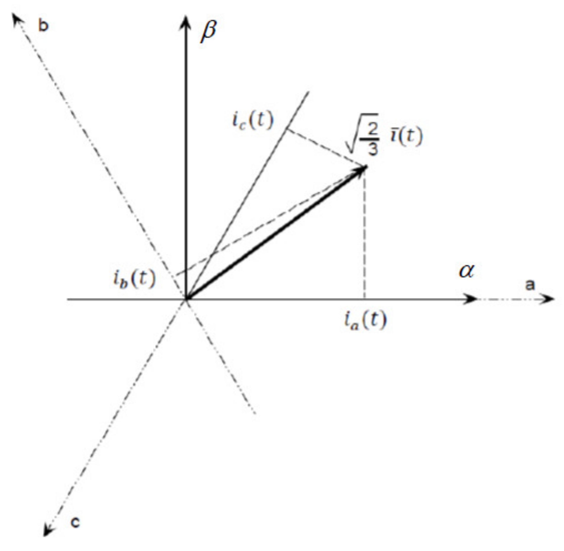Moreover, since the α and β modal circuits have the same topology and the same parameters (e.g., $L_{\alpha }=L_{\beta }$, as shown above), each couple of α and β electrical variables can be combined in a space vector, i.e., a complex valued function of time where the real part is given by the α component, and the imaginary part is given by the β component. For the currents in Equation (1), the corresponding space vector is defined as:

$$\overline{i}\left(t\right)=i_{\alpha }\left(t\right)+j{i}_{\beta }\left(t\right)$$

(3)

It can be readily shown that the phase variables a, b, c can be recovered from the space vector as:

$$i_a\left(t\right)=\sqrt{\frac{2}{3}}\mathrm{Re}\left(\overline{i}\left(t\right)\right)+\frac{1}{\sqrt{3}}{i}_0\left(t\right)$$

(4)

$$i_b\left(t\right)=\sqrt{\frac{2}{3}}\mathrm{Re}\left({\overline{\alpha }}^2\overline{i}\left(t\right)\right)+\frac{1}{\sqrt{3}}{i}_0\left(t\right)$$

(5)

$$i_c\left(t\right)=\sqrt{\frac{2}{3}}\mathrm{Re}\left(\overline{\alpha }\overline{i}\left(t\right)\right)+\frac{1}{\sqrt{3}}{i}_0\left(t\right)$$

(6)

where $\overline{\alpha }=e^{j2\pi /3}$. Therefore, apart from the zero component contribution $i_0\left(t\right)$, the phase variables a, b, c can be recovered as the instantaneous components of the space vector on the three axes denoted as a, b, and c on the complex plane, each with an angular displacement of $2\pi /3$ (see Figure 1).

In previous papers, it was shown that the use of Clarke transformation (similarly to the symmetrical components transformation) also results in topological properties of the modal circuits [33]. In particular, it was shown that: (1) in the α and β modal circuits, the star centers in a three-phase circuit correspond to shorted terminals with respect to the system reference point; (2) a single-phase circuit, possibly connected to the three-phase star centers, results in ideal transformers (with ratio $\sqrt{3}$) connecting such a single-phase circuit to the 0 modal circuit.

If the assumption of circuit symmetry of the three phases is not met, the use of the Clarke transformation does not provide matrix diagonalization. Therefore, the modal circuits α, β, and 0 are not uncoupled. Thus, in the conventional analysis, in case of phase asymmetry, the Clarke transformation is not used since its application does not lead to circuit simplification.

In this paper, however, it will be shown that a proper methodology can be defined in order to study single-line and double-line switching (i.e., circuit asymmetry) by using the Clarke transformation. The mutual coupling between modal circuits will be described in rigorous terms and a consistent circuit representation of circuit coupling will be derived.

Finally, it is worth noting that the Clarke transformation, as a linear transformation, can be used to operate in the Laplace domain. This property will be exploited in the transient analysis derived in the next section. The explicit time-domain solution of the proposed circuit models can be obtained through an inverse Laplace transformation.

3. Circuit Modeling of Line Switching for Transient Analysis: Laplace-Domain Approach

Single-line or double-line switching (i.e., opening or closing operation on one or two phases) in a three-phase circuit results in the loss of the main assumption for the effective use of the Clarke transformation, i.e., the circuit symmetry of the three phases. Therefore, the cases of single-line or double-line switching cannot be treated in a straightforward way through the Clarke transformation.

The proposed methodology foresees two steps [16], conceptually similar to the standard methodology used to analyze steady-state asymmetrical faults through symmetrical components in the phasor domain [3]. First, the three-phase section where the line switching is located is removed. Since the remaining three-phase circuit has phase symmetry, the Clarke transformation can be used and the three Thevenin equivalents α, β, and 0 in the Laplace domain can be derived. Second, the voltage/current constraints describing line switching are transformed into the Clarke domain, and the resulting constraints on the α, β, and 0 variables are implemented in the α, β, and 0 Thevenin equivalents previously obtained.

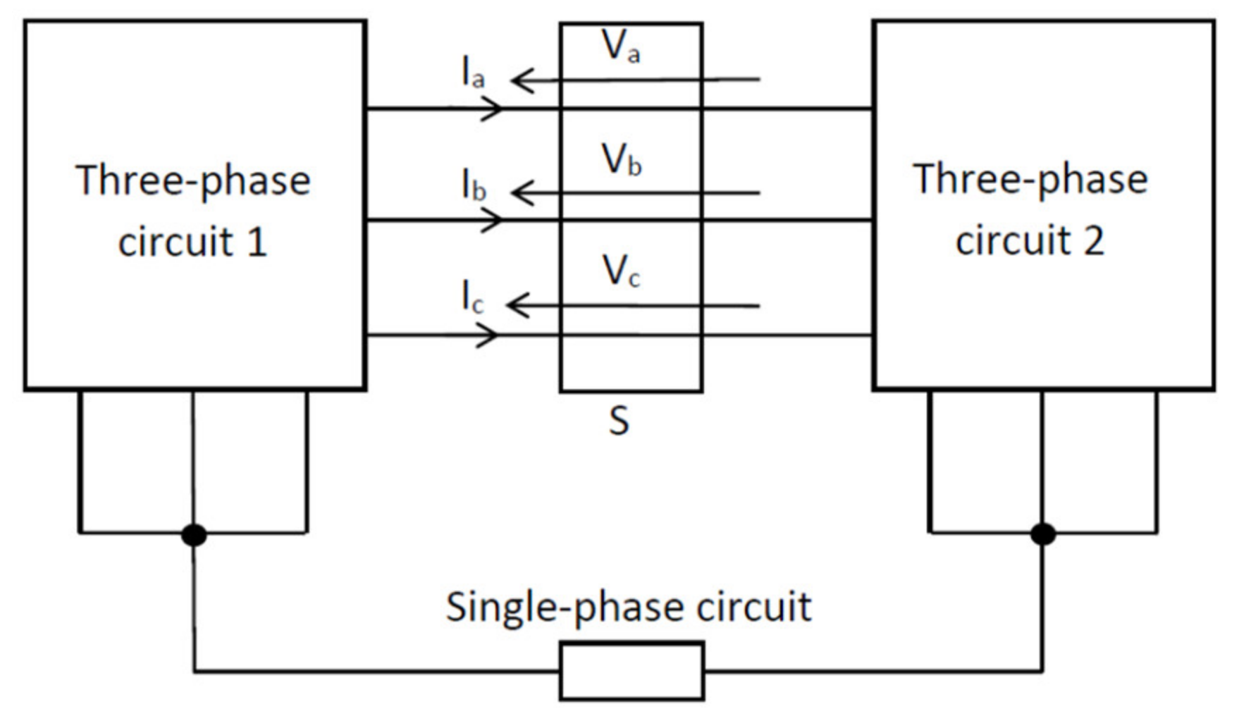
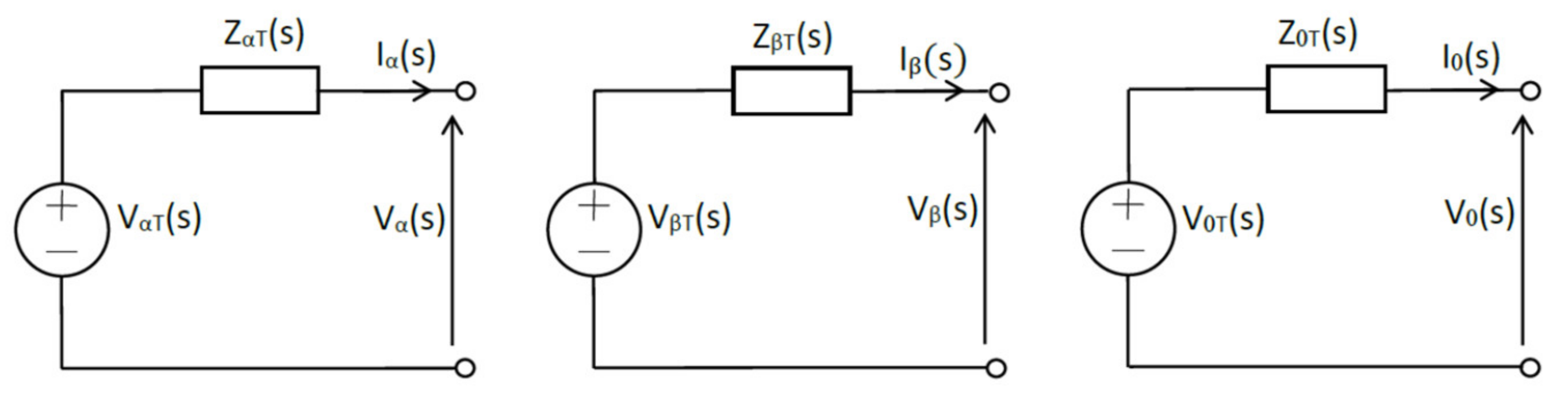
Let us consider the general three-phase circuit represented in Figure 2. A single-phase circuit connected across the star centers is also included. In the simplest case, such a single-phase circuit consists in an impedance (open and short circuits as special cases). The three-phase port (i.e., three-port component) S is the circuit representation of the three-phase section where line switching is located. As a three-port component, S will be defined by three relationships describing line switching (one or two lines involved). The methodology outlined above foresees first the removal of S in order to obtain the three-phase system with phase symmetry represented in Figure 3. Such a system can be studied with the conventional analysis based on the Clarke transformation. In particular, the α, β, and 0 Thevenin equivalents in the Laplace domain can be readily derived (Figure 4). The second step foresees the Clarke transformation and circuit implementation of the relationships describing the three-phase port S. To this aim, two cases can be considered, i.e., single-line switching (phase a), and double- line switching (phases b and c). For more general results, each line switch is modelled as an impedance Z (s) in parallel with an ideal switch opening at $t=0$ (Figure 5). Of course, the special case of ideal line interruption (i.e., open-circuit fault) can be modeled by assuming $Z\to \infty$.

It is worth noticing that the selection of phase a for single-line switching, and phases b and c for double-line switching have no impact on the generality of the following derivations. In fact, the analysis of a three-phase circuit can be always performed by renaming (if needed) the phases according to the choice operated in this paper.

3.1. Single-Line Switching

In case of line switching of phase a, the three-phase port S is described by the three Laplace-domain relationships:

$$I_a\left(s\right)=V_a\left(s\right)/Z\left(s\right),\hspace{1em}\hspace{1em}\hspace{1em}{V}_b\left(s\right)=0,\hspace{1em}\hspace{1em}\hspace{1em}{V}_c\left(s\right)=0$$

(7)

The Clarke transformation of Equation (7) provides:

$$\left[\begin{array}{c}{V}_{\alpha }\left(s\right)\\ V_{\beta }\left(s\right)\\ V_0\left(s\right)\end{array}\right]=\mathit{T}\left[\begin{array}{c}{V}_a\left(s\right)\\ 0\\ 0\end{array}\right]=\sqrt{\frac{2}{3}}\left[\begin{array}{c}{V}_a\left(s\right)\\ 0\\ V_a\left(s\right)/\sqrt{2}\end{array}\right]$$

(8)

$$\left[\begin{array}{c}{I}_{\alpha }\left(s\right)\\ I_{\beta }\left(s\right)\\ I_0\left(s\right)\end{array}\right]=\mathit{T}\left[\begin{array}{c}{V}_a\left(s\right)/Z\left(s\right)\\ I_b\left(s\right)\\ I_c\left(s\right)\end{array}\right]=\sqrt{\frac{2}{3}}\left[\begin{array}{c}{V}_a\left(s\right)/Z\left(s\right)-1/2\left(I_b\left(s\right)+I_c\left(s\right)\right)\\ \sqrt{3}/2\left(I_b\left(s\right)-I_c\left(s\right)\right)\\ 1/\sqrt{2}\left(V_a\left(s\right)/Z\left(s\right)+I_b\left(s\right)+I_c\left(s\right)\right)\end{array}\right]$$

(9)

From (8) we obtain

$$V_{\alpha }\left(s\right)=\sqrt{2}{V}_0\left(s\right)$$

(10)

whereas from Equation (9) by eliminating $\left(I_b\left(s\right)+I_c\left(s\right)\right)$, and by taking into account that from Equation (8) we have $V_a\left(s\right)=\sqrt{3/2}{V}_{\alpha }\left(s\right)$, we obtain

$$I_{\alpha }\left(s\right)=-\frac{1}{\sqrt{2}}{I}_0\left(s\right)+\frac{V_{\alpha }\left(s\right)}{\frac{2}{3}Z\left(s\right)}$$

(11)

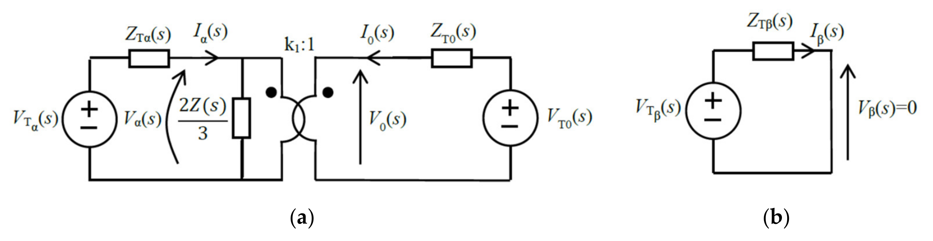
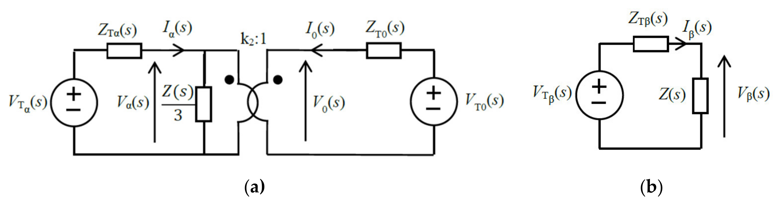
Therefore, from Equations (10) and (11), we obtain that the line switching of phase a results in circuit coupling between α and 0 Thevenin equivalents through an ideal transformer with ratio $k_1=\sqrt{2}$, and a parallel impedance $2Z\left(s\right)/3$ on the primary side (see Figure 6a). It is worth noticing that in the case of open 0 circuit (i.e., in case of missing fourth wire in the three-phase circuit), the α Thevenin circuit has an uncoupled transient with load $2Z\left(s\right)/3$.

Moreover, from Equation (8), we obtain $V_{\beta }\left(s\right)=0$, i.e., the β Thevenin equivalent is shorted and uncoupled with the other two Thevenin equivalents (Figure 6b). It is worth noting that the shorted β Thevenin circuit has no transient, i.e., it holds the previous steady state.

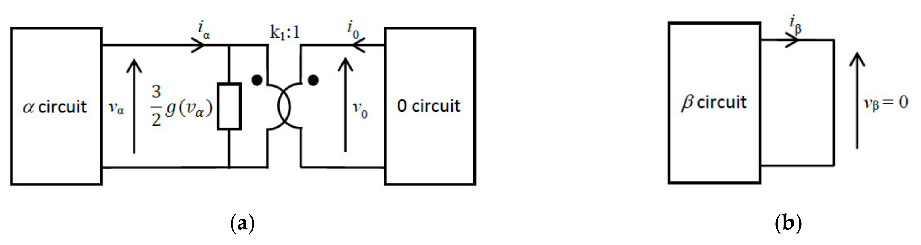
The modal variables α, β, 0 can be readily obtained by direct solution of the circuits in Figure 6:

$$V_{\alpha }\left(s\right)=\frac{\frac{V_{T\alpha }\left(s\right)}{Z_{T\alpha }\left(s\right)}+\frac{k_1{V}_{T0}\left(s\right)}{k_1^2{Z}_{T0}\left(s\right)}}{\frac{1}{Z_{T\alpha }\left(s\right)}+\frac{1}{\frac{2}{3}Z\left(s\right)}+\frac{1}{k_1^2{Z}_{T0}\left(s\right)}}$$

(12)

$$V_0\left(s\right)=\frac{1}{k_1}{V}_{\alpha }\left(s\right)$$

(13)

$$V_{\beta }\left(s\right)=0$$

(14)

$$I_{\alpha }\left(s\right)=\frac{V_{T\alpha }\left(s\right)-V_{\alpha }\left(s\right)}{Z_{T\alpha }\left(s\right)}$$

(15)

$$I_0\left(s\right)=-k_1\left(I_{\alpha }\left(s\right)-\frac{V_{\alpha }\left(s\right)}{\frac{2}{3}Z\left(s\right)}\right)$$

(16)

$$I_{\beta }\left(s\right)=\frac{V_{T\beta }\left(s\right)}{Z_{T\beta }\left(s\right)}$$

(17)

where $I_{\beta }$ is not affected by the line switching.

As far as the phase voltage $V_a\left(s\right)$ is concerned, from the inverse Clarke transformation we obtain:

$$V_a\left(s\right)=\sqrt{\frac{2}{3}}{V}_{\alpha }\left(s\right)+\frac{1}{\sqrt{3}}{V}_0\left(s\right)=\sqrt{\frac{3}{2}}{V}_{\alpha }\left(s\right)$$

(18)

Finally, from the inverse Clarke transformation, the phase currents can be obtained:

$$\left[\begin{array}{c}{I}_a\left(s\right)\\ I_b\left(s\right)\\ I_c\left(s\right)\end{array}\right]={\mathit{T}}^{-\mathbf{1}}\left[\begin{array}{c}{I}_{\alpha }\left(s\right)\\ I_{\beta }\left(s\right)\\ I_0\left(s\right)\end{array}\right]$$

(19)

In particular, after simple algebra we obtain:

$$I_a\left(s\right)=\sqrt{\frac{3}{2}}\frac{V_{\alpha }\left(s\right)}{Z\left(s\right)}$$

(20)

$$I_b\left(s\right)=\sqrt{\frac{3}{2}}\left(-I_{\alpha }\left(s\right)+\frac{1}{\sqrt{3}}{I}_{\beta }\left(s\right)+\frac{1}{Z\left(s\right)}{V}_{\alpha }\left(s\right)\right)$$

(21)

$$I_c\left(s\right)=\sqrt{\frac{3}{2}}\left(-I_{\alpha }\left(s\right)-\frac{1}{\sqrt{3}}{I}_{\beta }\left(s\right)+\frac{1}{Z\left(s\right)}{V}_{\alpha }\left(s\right)\right)$$

(22)

Note that in case of ideal line interruption (i.e., $Z\to \infty$), from Equation (20), we obtain consistently that the current in phase a is zero (open-circuit fault).

The time-domain solutions can be obtained through conventional inverse Laplace transform of Equations (12)–(18), and (20)–(22). Thus, explicit time-domain solutions depend on the parameters of the Thevenin equivalents of the specific circuit under analysis.

3.2. Double-Line Switching

In the case of simultaneous line switching of phases b and c, and by assuming equal impedances Z, the three-phase port S is described by these three relationships:

$$V_a\left(s\right)=0, I_b\left(s\right)=V_b\left(s\right)/Z\left(s\right), I_c\left(s\right)=V_c\left(s\right)/Z\left(s\right)$$

(23)

The Clarke transformation of Equations (23) provides:

$$\left[\begin{array}{c}{V}_{\alpha }\left(s\right)\\ V_{\beta }\left(s\right)\\ V_0\left(s\right)\end{array}\right]=\mathit{T}\left[\begin{array}{c}0\\ V_b\left(s\right)\\ V_c\left(s\right)\end{array}\right]=\sqrt{\frac{2}{3}}\left[\begin{array}{c}-1/2\left(V_b\left(s\right)+V_c\left(s\right)\right)\\ \sqrt{3}/2\left(V_b\left(s\right)-V_c\left(s\right)\right)\\ 1/\sqrt{2}\left(V_b\left(s\right)+V_c\left(s\right)\right)\end{array}\right]$$

(24)

$$\left[\begin{array}{c}{I}_{\alpha }\left(s\right)\\ I_{\beta }\left(s\right)\\ I_0\left(s\right)\end{array}\right]=\mathit{T}\left[\begin{array}{c}{I}_a\left(s\right)\\ V_b\left(s\right)/Z\left(s\right)\\ V_c\left(s\right)/Z\left(s\right)\end{array}\right]=\sqrt{\frac{2}{3}}\left[\begin{array}{c}{I}_a\left(s\right)-\frac{1}{2Z\left(s\right)}\left(V_b\left(s\right)+V_c\left(s\right)\right)\\ \frac{\sqrt{3}}{2Z\left(s\right)}\left(V_b\left(s\right)-V_c\left(s\right)\right)\\ \frac{1}{\sqrt{2}}\left(I_a\left(s\right)+\frac{V_b\left(s\right)+V_c\left(s\right)}{Z\left(s\right)}\right)\end{array}\right]$$

(25)

From Equation (24), we obtain:

$$V_{\alpha }\left(s\right)=-\frac{1}{\sqrt{2}}{V}_0\left(s\right)$$

(26)

whereas by eliminating $I_a$ in Equation (25) and by taking into account that from Equation (24), we have $V_{\alpha }\left(s\right)=-\frac{V_b\left(s\right)+V_c\left(s\right)}{\sqrt{6}}$, we obtain:

$$I_{\alpha }\left(s\right)=\sqrt{2}{I}_0\left(s\right)+\frac{V_{\alpha }\left(s\right)}{Z\left(s\right)/3}$$

(27)

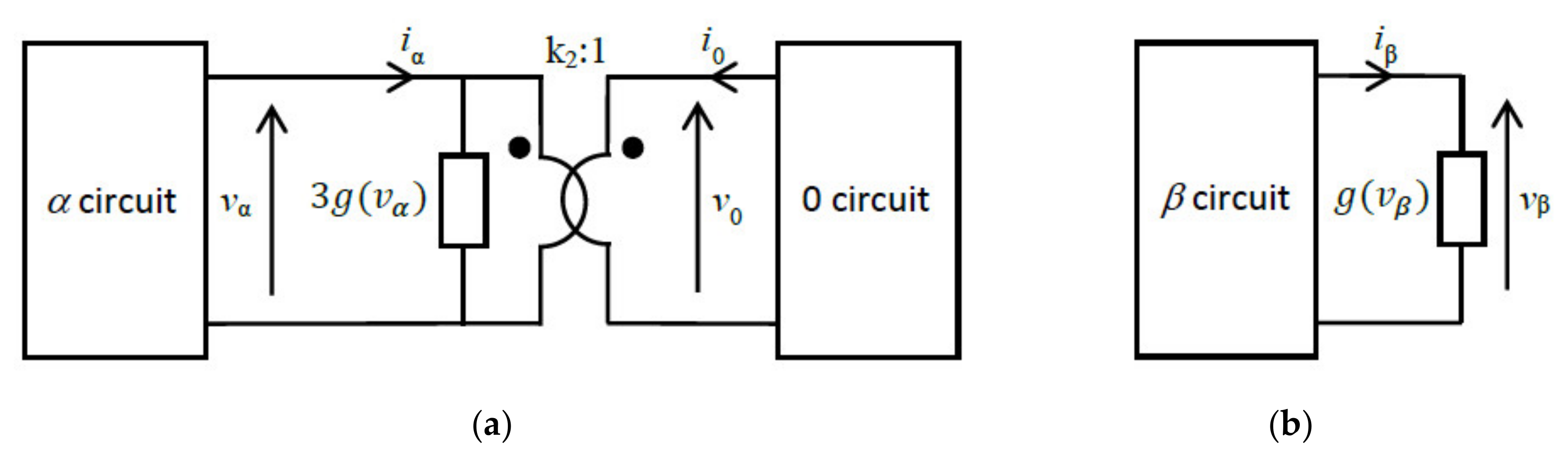
From Equations (26) and (27) we readily obtain that the two modal circuits α and 0 are coupled through an ideal transformer with ratio $k_2=-\frac{1}{\sqrt{2}}$, and a parallel impedance $Z\left(s\right)/3$ on the primary side (Figure 7a). In the special case of a missing fourth wire (i.e., no single-phase circuit across the star centers), the 0 circuit is open and the α circuit shows an uncoupled transient behavior with load $Z\left(s\right)/3$.

Moreover, from Equations (24) and (25), we obtain $V_{\beta }\left(s\right)=Z\left(s\right)I_{\beta }\left(s\right)$, i.e., the β Thevenin equivalent has the load impedance Z, and it is uncoupled with the other two modal circuits (Figure 7b). Notice that, contrary to the single-line case where the β circuit had no transient, in this case also the β circuit shows a transient behavior.

The modal variables can be readily evaluated from the equivalent circuits in Figure 7a,b. The analysis provides results similar to Equations (12)–(17):

$$V_{\alpha }\left(s\right)=\frac{\frac{V_{T\alpha }\left(s\right)}{Z_{T\alpha }\left(s\right)}+\frac{k_2{V}_{T0}\left(s\right)}{k_2^2{Z}_{T0}\left(s\right)}}{\frac{1}{Z_{T\alpha }\left(s\right)}+\frac{1}{\frac{1}{3}Z\left(s\right)}+\frac{1}{k_2^2{Z}_{T0}\left(s\right)}}$$

(28)

$$V_0\left(s\right)=\frac{1}{k_2}{V}_{\alpha }\left(s\right)$$

(29)

$$V_{\beta }\left(s\right)=V_{T\beta }\left(s\right)\frac{Z\left(s\right)}{Z_{T\beta }\left(s\right)+Z\left(s\right)}$$

(30)

$$I_{\alpha }\left(s\right)=\frac{V_{T\alpha }\left(s\right)-V_{\alpha }\left(s\right)}{Z_{T\alpha }\left(s\right)}$$

(31)

$$I_0\left(s\right)=-k_2\left(I_{\alpha }\left(s\right)-\frac{V_{\alpha }\left(s\right)}{\frac{1}{3}Z\left(s\right)}\right)$$

(32)

$$I_{\beta }\left(s\right)=\frac{V_{T\beta }\left(s\right)}{Z_{T\beta }\left(s\right)+Z\left(s\right)}$$

(33)

From the inverse Clarke transformation, we obtain the phase voltages:

$$\left[\begin{array}{c}{V}_a\left(s\right)\\ V_b\left(s\right)\\ V_c\left(s\right)\end{array}\right]={\mathit{T}}^{-1}\left[\begin{array}{c}{V}_{\alpha }\left(s\right)\\ V_{\beta }\left(s\right)\\ V_0\left(s\right)\end{array}\right]$$

(34)

In particular, from Equations (28)–(30), we have the obvious result $V_a\left(s\right)=0$, and:

$$V_b\left(s\right)=\sqrt{\frac{3}{2}}\left(-V_{\alpha }\left(s\right)+\frac{1}{\sqrt{3}}{V}_{\beta }\left(s\right)\right)$$

(35)

$$V_c\left(s\right)=\sqrt{\frac{3}{2}}\left(-V_{\alpha }\left(s\right)-\frac{1}{\sqrt{3}}{V}_{\beta }\left(s\right)\right)$$

(36)

Finally, also the phase currents can be readily obtained by the inverse Clarke transformation (19). After simple algebra, we obtain:

$$I_a\left(s\right)=\sqrt{\frac{3}{2}}\left(I_{\alpha }\left(s\right)-\frac{1}{Z\left(s\right)}{V}_{\alpha }\left(s\right)\right)$$

(37)

$$I_b\left(s\right)=\sqrt{\frac{3}{2}}\left(\frac{1}{\sqrt{3}}{I}_{\beta }\left(s\right)-\frac{1}{Z\left(s\right)}{V}_{\alpha }\left(s\right)\right)$$

(38)

$$I_c\left(s\right)=\sqrt{\frac{3}{2}}\left(-\frac{1}{\sqrt{3}}{I}_{\beta }\left(s\right)-\frac{1}{Z\left(s\right)}{V}_{\alpha }\left(s\right)\right)$$

(39)

Notice that in the case of ideal line interruptions (i.e., $Z\to \infty$ on phases b and c) both $I_b\left(s\right)$ and $I_c\left(s\right)$ approach zero, since also $I_{\beta }\left(s\right)\to 0$ (see Equation (33)).

The time-domain solutions can be obtained through conventional inverse Laplace transform of Equations (28)–(33) and (35)–(39).

4. Circuit Modeling of Line Switching for Transient Analysis: Time-Domain Approach

The Laplace-domain analysis derived in Section 3 can be readily reformulated in the time domain to obtain transient solutions in explicit form. In the Laplace domain, each line switch was modeled as an ideal switch in parallel with an impedance $Z\left(s\right)$ (see Figure 5). In the time domain, we assume that the element in parallel with each ideal switch has a voltage/current relationship of the form $i=g\left(v\right)$, where $g$, in general, is a linear integral/differential relationship. For example, in case of a parallel connection of a resistor and a capacitor, $i=g\left(v\right)=Gv+Cdv/dt$. This assumption is needed since in the following derivations the phase currents must be written in terms of voltages.

The two cases of single-line and double-line switching will be considered. In both cases, for $t<0$, the α, β, and 0 dynamic circuits are uncoupled since the three switches are still closed. For $t\ge 0$ the three-phase port S sets single or double-phase constraints on the phase variables. In the following subsections, it is shown that such constraints correspond to coupling between α and 0 circuits through an ideal transformer with different transformation ratio for single and double-line switching.

4.1. Single-Line Switching

In the case of line switching in $t=0$ of phase a, the three-phase port S is described for $t\ge 0$ by the three time-domain relationships:

$$i_a\left(t\right)=g\left(v_a\left(t\right)\right), v_b\left(t\right)=0, v_c\left(t\right)=0$$

(40)

The Clarke transformation of Equations (40) provides:

$$\left[\begin{array}{c}{v}_{\alpha }\\ v_{\beta }\\ v_0\end{array}\right]=\mathit{T}\left[\begin{array}{c}{v}_a\\ 0\\ 0\end{array}\right]=\sqrt{\frac{2}{3}}\left[\begin{array}{c}{v}_a\\ 0\\ v_a/\sqrt{2}\end{array}\right]$$

(41)

$$\left[\begin{array}{c}{i}_{\alpha }\\ i_{\beta }\\ i_0\end{array}\right]=\mathit{T}\left[\begin{array}{c}g\left(v_a\right)\\ i_b\\ i_c\end{array}\right]=\sqrt{\frac{2}{3}}\left[\begin{array}{c}g\left(v_a\right)-1/2\left(i_b+i_c\right)\\ \sqrt{3}/2\left(i_b-i_c\right)\\ 1/\sqrt{2}\left(g\left(v_a\right)+i_b+i_c\right)\end{array}\right]$$

(42)

From Equation (41) we obtain

$$v_{\alpha }=\sqrt{2}{v}_0$$

(43)

whereas from Equation (42) by eliminating $\left(i_b+i_c\right)$, and by taking into account that from Equation (41) we have $v_a=\sqrt{3/2}{v}_{\alpha }$, we obtain

$$i_{\alpha }=-\frac{1}{\sqrt{2}}{i}_0+\frac{3}{2}g\left(v_{\alpha }\right)$$

(44)

Therefore, from Equations (43) and (44) we obtain that the line switching of phase a results in circuit coupling between α and 0 circuits through an ideal transformer with ratio $k_1=\sqrt{2}$, and a parallel element with current $\frac{3}{2}g\left(v_{\alpha }\right)$ on the primary side (see Figure 8a). It is worth noticing that in the case of an open 0 circuit (i.e., in the case of a missing fourth wire in the three-phase circuit), the α circuit has an uncoupled transient with load $\frac{3}{2}g\left(v_{\alpha }\right)$. This result is the time-domain version of the Laplace-domain result where the parallel element on the primary side of the ideal transformer was the impedance $\frac{2}{3}Z\left(s\right)$.

Moreover, from Equation (41) we obtain $v_{\beta }=0$, i.e., the β circuit is shorted and uncoupled with the other two circuits (Figure 8b). It is worth noticing that the shorted β circuit has no transient, i.e., it holds the previous steady state.

4.2. Double-Line Switching

In the case of simultaneous line switching of phases b and c, and by assuming an equal voltage/current relationship $i=g\left(v\right)$ for the elements in parallel to ideal switches, the three-phase port S is described by the three relationships:

$$v_a=0, i_b=g\left(v_b\right), i_c=g\left(v_c\right)$$

(45)

The Clarke transformation of Equation (45) provides:

$$\left[\begin{array}{c}{v}_{\alpha }\\ v_{\beta }\\ v_0\end{array}\right]=\mathit{T}\left[\begin{array}{c}0\\ v_b\\ v_c\end{array}\right]=\sqrt{\frac{2}{3}}\left[\begin{array}{c}-1/2\left(v_b+v_c\right)\\ \sqrt{3}/2\left(v_b-v_c\right)\\ 1/\sqrt{2}\left(v_b+v_c\right)\end{array}\right]$$

(46)

$$\left[\begin{array}{c}{i}_{\alpha }\\ i_{\beta }\\ i_0\end{array}\right]=\mathit{T}\left[\begin{array}{c}{i}_a\\ g\left(v_b\right)\\ g\left(v_c\right)\end{array}\right]=\sqrt{\frac{2}{3}}\left[\begin{array}{c}{i}_a-\frac{1}{2}\left(g\left(v_b\right)+g\left(v_c\right)\right)\\ \frac{\sqrt{3}}{2}\left(g\left(v_b\right)-g\left(v_c\right)\right)\\ \frac{1}{\sqrt{2}}\left(i_a+g\left(v_b\right)+g\left(v_c\right)\right)\end{array}\right]$$

(47)

From Equation (46) we obtain:

$$v_{\alpha }=-\frac{1}{\sqrt{2}}{v}_0$$

(48)

whereas by eliminating $i_a$ in Equation (47), by taking into account that from Equation (46), we have $v_{\alpha }=-\frac{v_b+v_c}{\sqrt{6}}$, and by using the linearity assumption $g\left(v_a\right)+g\left(v_b\right)=g\left(v_a+v_b\right)$, we obtain:

$$i_{\alpha }=\sqrt{2}{i}_0+3g\left(v_{\alpha }\right)$$

(49)

From Equations (48) and (49) we readily obtain that the two modal circuits α and 0 are coupled through an ideal transformer with ratio $k_2=-\frac{1}{\sqrt{2}}$, and a parallel element with current $3g\left(v_{\alpha }\right)$ on the primary side (Figure 9a). In the special case of a missing fourth wire (i.e., no single-phase circuit across the star centers), the 0 circuit is open and the α circuit shows an uncoupled transient behavior with load $3g\left(v_{\alpha }\right)$. This result is the time-domain version of the Laplace-domain result where the parallel element on the primary side of the ideal transformer was the impedance $\frac{1}{3}Z\left(s\right)$.

Moreover, from Equations (46) and (47) we obtain $i_{\beta }=g\left(v_{\beta }\right)$, i.e., the β circuit is loaded with the element $g\left(v\right)$, and it is uncoupled with the other two modal circuits (Figure 9b). Notice that, contrary to the single-line case where the β circuit had no transient, in this case also the β circuit shows a transient behavior.

4.3. Time-Domain Analytical Solution

The dynamic circuits in Figure 8 and Figure 9 can be readily solved in the time domain through the conventional state-equation approach. Given a three-phase circuit with dynamic order N, the total dynamic order after Clarke transformation must still be N. Thanks to the decoupling of the β circuit, however, each circuit in Figure 8 and Figure 9 (i.e., the α-0 circuit and the β circuit) typically has a dynamic order $N/2$. Thus, the proposed methodology allows the analytical evaluation of transients by solving dynamic circuits with half dynamic order with respect to the original three-phase circuit. Moreover, in the case of single-line switching, it was shown that the β circuit has no transient. Therefore, only the α-0 circuit must be solved.

More specifically, each circuit in Figure 8 and Figure 9, with dynamic order M, can be described in terms of a state equation of the form:

$$\frac{d}{dt}\mathit{x}=\mathit{A}\mathit{x}+\mathit{B}\mathit{u}$$

(50)

where x is the column vector of the M state variables, u is the column vector of the sources, A is the M × M state matrix, and B is the input matrix. For sinusoidal sources with angular frequency $\omega$, the steady-state solution is given by the phasor solution:

$${\mathit{X}}_s={\left(j\omega \mathbf{1}-\mathit{A}\right)}^{-1}\mathit{B}\mathit{U}$$

(51)

where 1 is the M × M identity matrix, and ${\mathit{X}}_s$ and $\mathit{U}$ are phasor vectors.

The transient component $x_t$ of the solution can be readily calculated from the eigenvalues ${\left\{{\lambda }_m\right\}}_{m=1}^M$ of the state matrix A. Indeed, by assuming distinct eigenvalues, the transient of the generic k-th state variable can be written as:

$$x_{t,k}\left(t\right)={\displaystyle \sum }_{m=1}^M{C}_{k,m}{e}^{{\lambda }_{m}t}$$

(52)

where the constants $C_{k,m}$ can be calculated by setting the initial conditions ${\mathit{x}}_0=\mathit{x}\left(0\right)-{\mathit{x}}_s\left(0\right)$ as [14]:

$$\mathit{C}=\left[\begin{array}{ccc}{C}_{1,1}& \cdots & C_{1,M}\\ ⋮& \ddots & ⋮\\ C_{M,1}& \cdots & C_{M,M}\end{array}\right]=\left[\begin{array}{llll}{\mathit{x}}_0& \mathit{A}{\mathit{x}}_0& \dots & {\mathit{A}}^{M-1}{\mathit{x}}_0\end{array}\right]{\left[\begin{array}{ccccc}1& {\lambda }_1& {\lambda }_1^2& \cdots & {\lambda }_1^{M-1}\\ ⋮& ⋮& ⋮& \cdots & ⋮\\ 1& {\lambda }_M& {\lambda }_M^2& \cdots & {\lambda }_M^{M-1}\end{array}\right]}^{-1}.$$

(53)

Therefore, the complete solution is given by:

$$\mathit{x}\left(t\right)={\mathit{x}}_t\left(t\right)+{\mathit{x}}_s\left(t\right)$$

(54)

5. Case Study

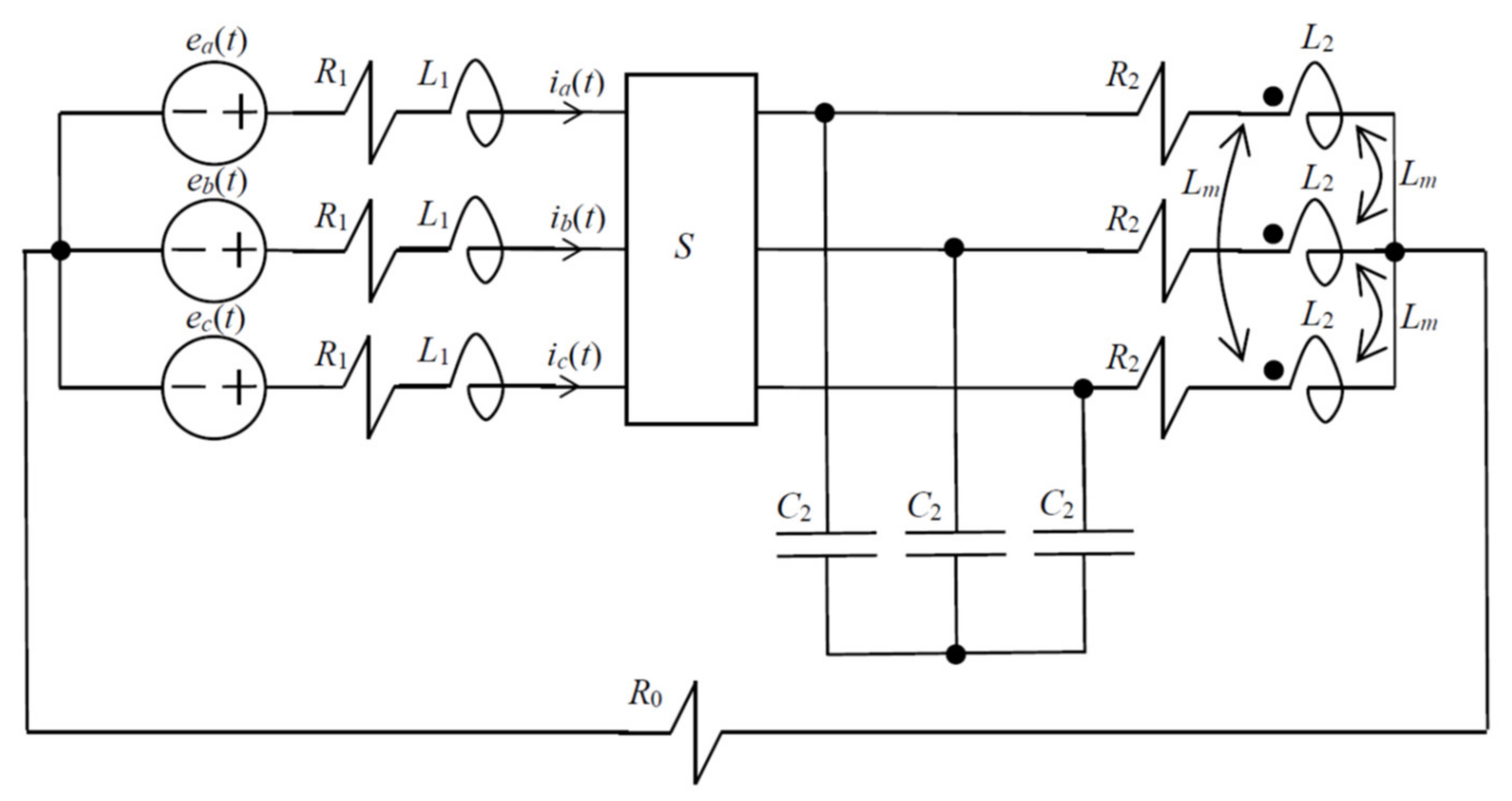
The simple three-phase circuit represented in Figure 10 was studied by means of the circuit models and the analytical results obtained in Section 3 and Section 4. The circuit was also implemented in Simulink/Matlab (R2020a, The MathWorks, Inc., Natick, MA, USA) to check the correctness of analytical results. The objective was the evaluation of the time-domain behavior of the phase currents $i_a\left(t\right), i_b\left(t\right), i_c\left(t\right)$, and the corresponding space vector $\overline{i}\left(t\right)$, caused by the line-switching operated by the three-phase port S.

Analytical evaluations were performed by implementing in Matlab the time-domain approach outlined in Section 4. The same results, however, can be obtained through the equivalent frequency-domain approach outlined in Section 3 by means of inverse Laplace transform. Notice that the dynamic order N of the three-phase circuit in Figure 10 is 8, increased by the dynamic order of the switching network S. By means of the methodology outlined in Section 4, however, the α-0 circuits in Figure 8 and Figure 9 have a dynamic order of 4, increased by the dynamic order of the switching element $g\left(v\right)$. The dynamic order of the β circuit is 4 in Figure 8, increased by the dynamic order of the switching element $g\left(v\right)$ in Figure 9. Thus, the original dynamic three-phase circuit has been split into uncoupled circuits with lower dynamic order.

In Figure 10, line switching is operated by the three-phase port S whose inner structure is represented in Figure 5a for the single-line case, and in Figure 5b for the double-line case. The impedance Z is assumed as consisting in the series connection of a capacitor C and a resistor R. The resistance $R_0$ of the single-phase circuit can be set to an extremely large value to implement the case of an open single-phase circuit.

The following numerical values were assumed for the parameters in Figure 10. Notice that the selected values have no specific relation with a practical system implementation, since the proposed case study is for illustration purposes only. The sinusoidal 50 Hz three-phase voltage source was selected such that the corresponding positive-sequence phasor is $E_p=100e^{j30°} \mathrm{V}$, the negative-sequence phasor is zero, and the zero-sequence phasor is $E_0=10\mathrm{V}$. The resistance parameters were $R_1=0.1 \mathsf{\Omega }$ and $R_2=10 \mathsf{\Omega }$. The fourth-wire resistance $R_0$ was set as equal to $1 \mathsf{\Omega }$ in simulations where the impact of the single-phase circuit was studied, and arbitrarily large in the case of an open single-phase circuit. The inductive/capacitive parameters were $L_1=1 \mathrm{mH}$, $L_2=20 \mathrm{mH}$, $L_m=5 \mathrm{mH}$, $C_2=122 \mathsf{\mu }\mathrm{F}$. Finally, different values were considered for the R and C line-switching parameters within the three-phase port S. In particular, $R=0$ and $R=1 \mathsf{\Omega }$ to put into evidence the role of R in damping oscillations, $C=100 \mathsf{\mu }\mathrm{F}$ and $C=500 \mathsf{\mu }\mathrm{F}$ to highlight the corresponding dynamical effects.

Figure 11, Figure 12, Figure 13 and Figure 14 were obtained for single-line switching, whereas Figure 15, Figure 16 and Figure 17 were obtained for double-line switching. 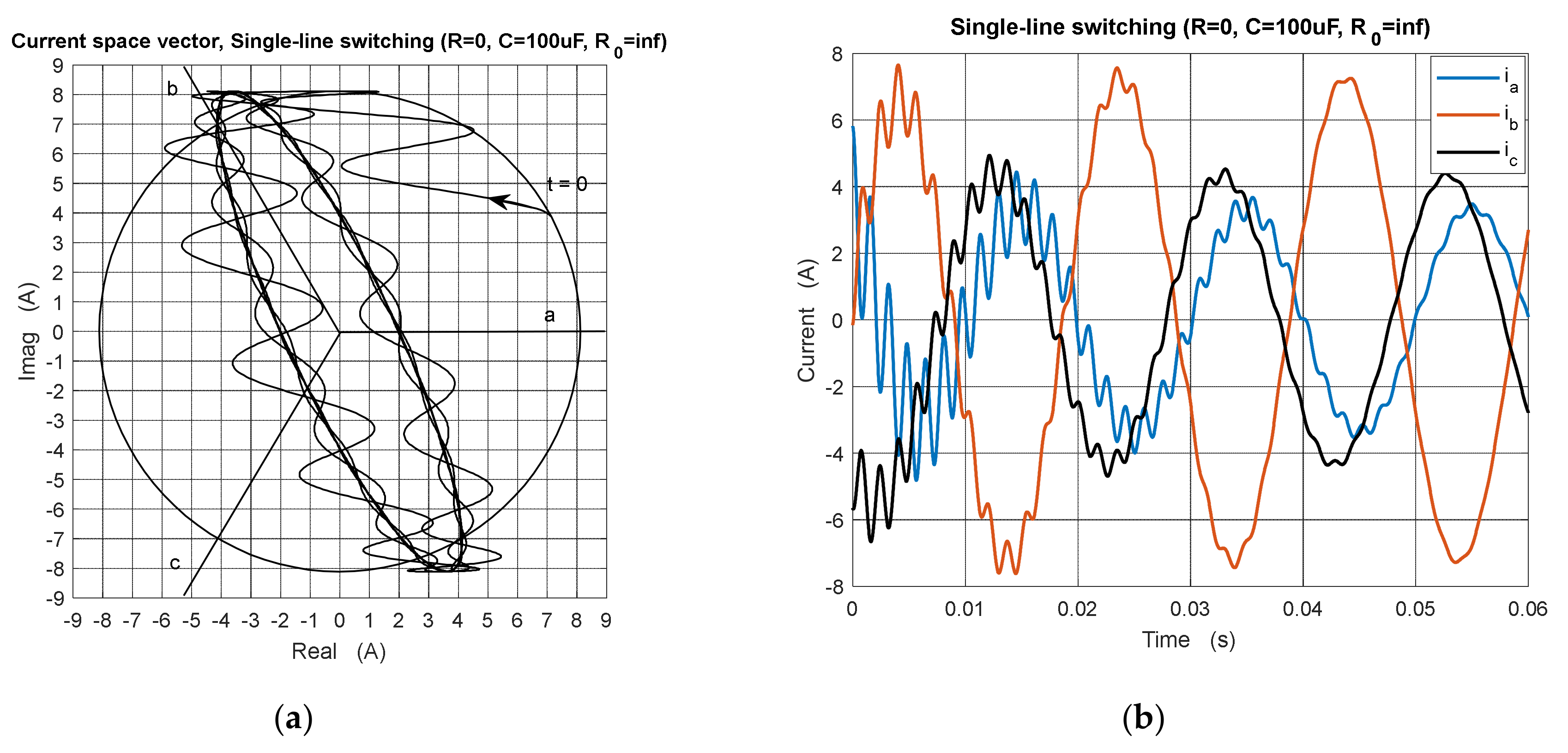All the figures show the time-domain behavior of the space vector $\overline{i}\left(t\right)$ on the complex plane (the figures denoted with letter (a)), and the corresponding phase currents $i_a\left(t\right), i_b\left(t\right), i_c\left(t\right)$ as functions of time (the figures denoted with letter (b)). In each figure, the current space vector is represented also for the steady state preceding the line switching occurring at $t=0$. Such steady-state trajectory is a circle because the voltage source has negative-sequence component equal to zero. The point denoted with $t=0$ on the complex plane is corresponding to the starting point of the transient, where the space vector trajectory leaves the circular shape.

Figure 11a,b shows the case of an open single-phase circuit, and single-line switching with $R=0$ and $C=100 \mathsf{\mu }\mathrm{F}$. Note the high-frequency oscillations captured by the analytical model. According to the modal circuits derived in Section 3 and Section 4, in this case the α circuit has an uncoupled transient (open single-phase circuit), whereas the β circuit has no transient because it is shorted (steady state). Thus, the high-frequency oscillations in Figure 11a (and the corresponding oscillations in Figure 11b) are due to the α component only (i.e., the x-coordinate), whereas the β component (i.e., the y-coordinate) is in steady state and is not affected by the line switching. That is why the high-frequency oscillations in Figure 11a have dominant horizontal direction (axis a). This explains the large relative amplitude of the high-frequency oscillations superimposed to $i_a\left(t\right)$ in Figure 11b. Moreover, notice that the angular orientation of the space vector trajectory in Figure 11a explains the dominant magnitude of the phase current b in Figure 11b since $i_b\left(t\right)$ is given by the space vector component on the axis b represented in Figure 11a.

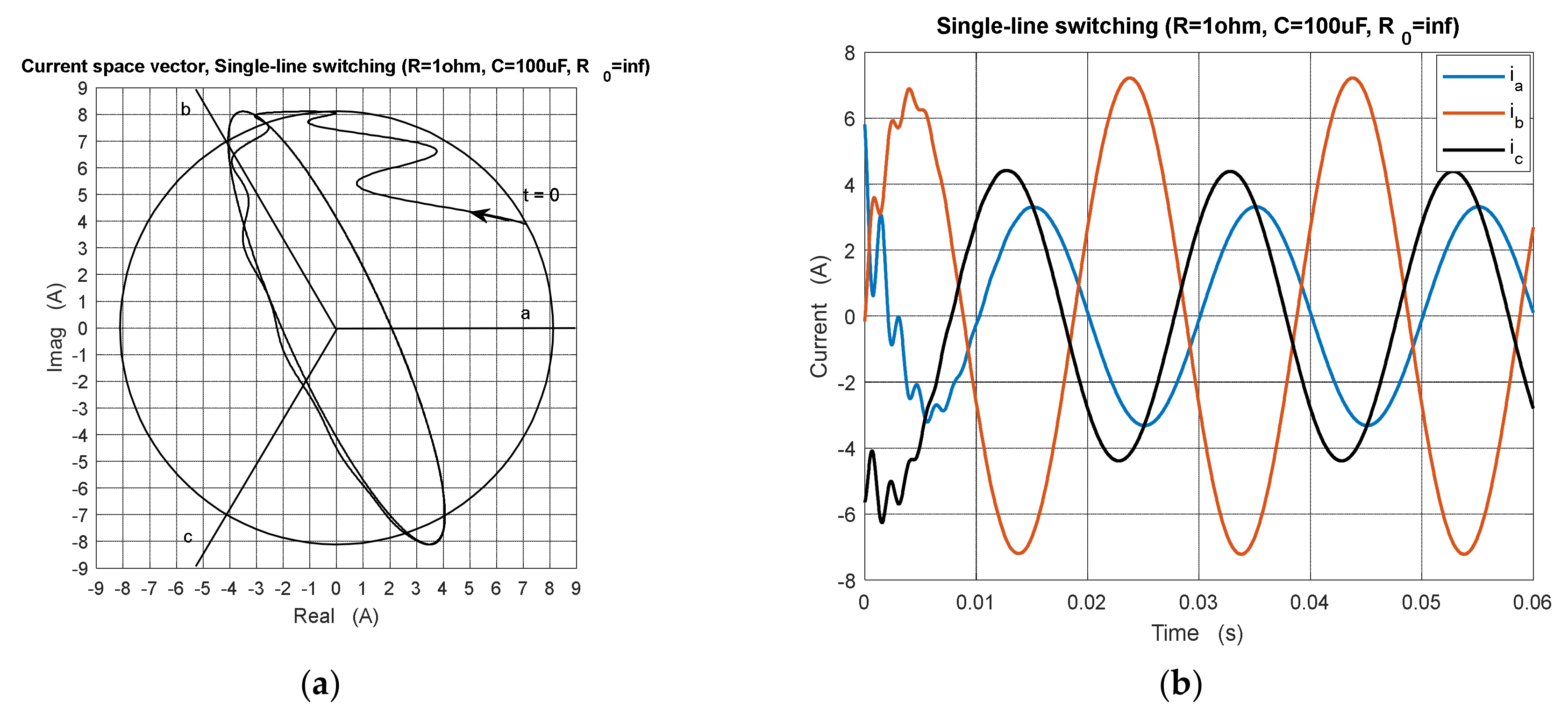
Figure 12a,b shows the effect of a resistor $R=1 \mathsf{\Omega }$ in series with the capacitor C in the line-switch impedance Z. Comparison with Figure 11a,b shows the damping effect of the resistor. In fact, oscillations are rapidly attenuated both in the space vector and in the phase currents. Notice that the ellipse in Figure 12a, corresponding to the new steady state, is fundamentally the same as in Figure 11a. This is because, according to Figure 6a, the load of the α circuit is $2Z/3$, where Z is dominated by the capacitive component at 50 Hz (i.e., $R\ll 1/\left(\omega C\right)$).

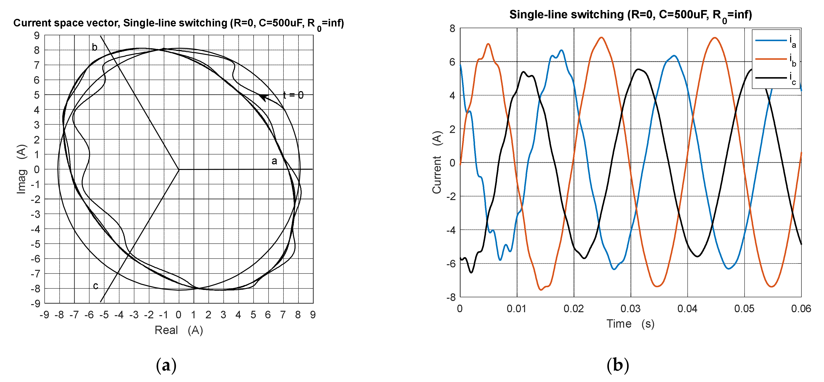
Figure 13a,b should be compared with Figure 11a,b since only the value of the capacitance C was changed to $C=500 \mathsf{\mu }\mathrm{F}$. Two main effects can be highlighted. First, the amplitude of the oscillations is smaller. Second, the ellipse in Figure 13a, corresponding to the new steady state, is wider than the ellipse in Figure 11a. This is due to the smaller impedance Z (i.e., larger capacitance C) forming the load of the α circuit. Thus, a wider excursion of the α component of the space vector results in a wider elliptical shape. Notice that the maximum range of the β component remains unchanged, since the β circuit is not affected by the line switch. As a result, the time-behavior of the phase currents represented in Figure 13b is more regular and shows closer peak values with respect to Figure 11b and Figure 12b.

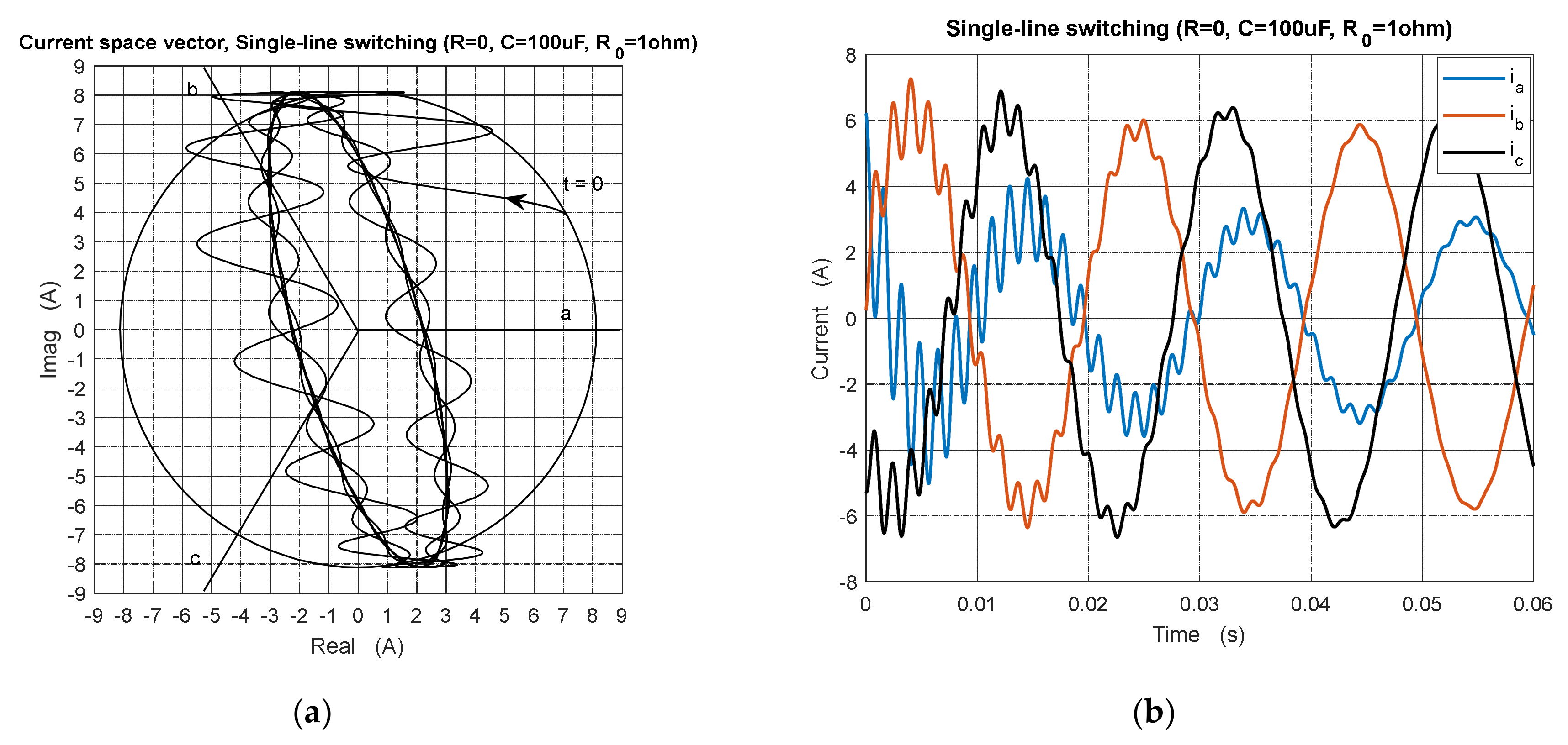
Figure 14a,b shows the effect of the interaction between the 0 and the α circuits. In fact, in this case the resistance of the single-phase circuit was set to $R_0=1 \mathsf{\Omega }$. According to the circuit model in Figure 6, in this case the transient of the α circuit is affected by the 0 circuit, whereas the β circuit is still in steady state. Actually, by comparing Figure 14a with Figure 11a, we observe a different inclination angle of the two ellipses, whereas the range of the β component is still unchanged. The small clockwise rotation of the space vector ellipse in Figure 14a with respect to Figure 11a results in a change in phase currents amplitude, i.e., a decreased amplitude for $i_a$ and closer amplitudes for $i_b$ and $i_c$.

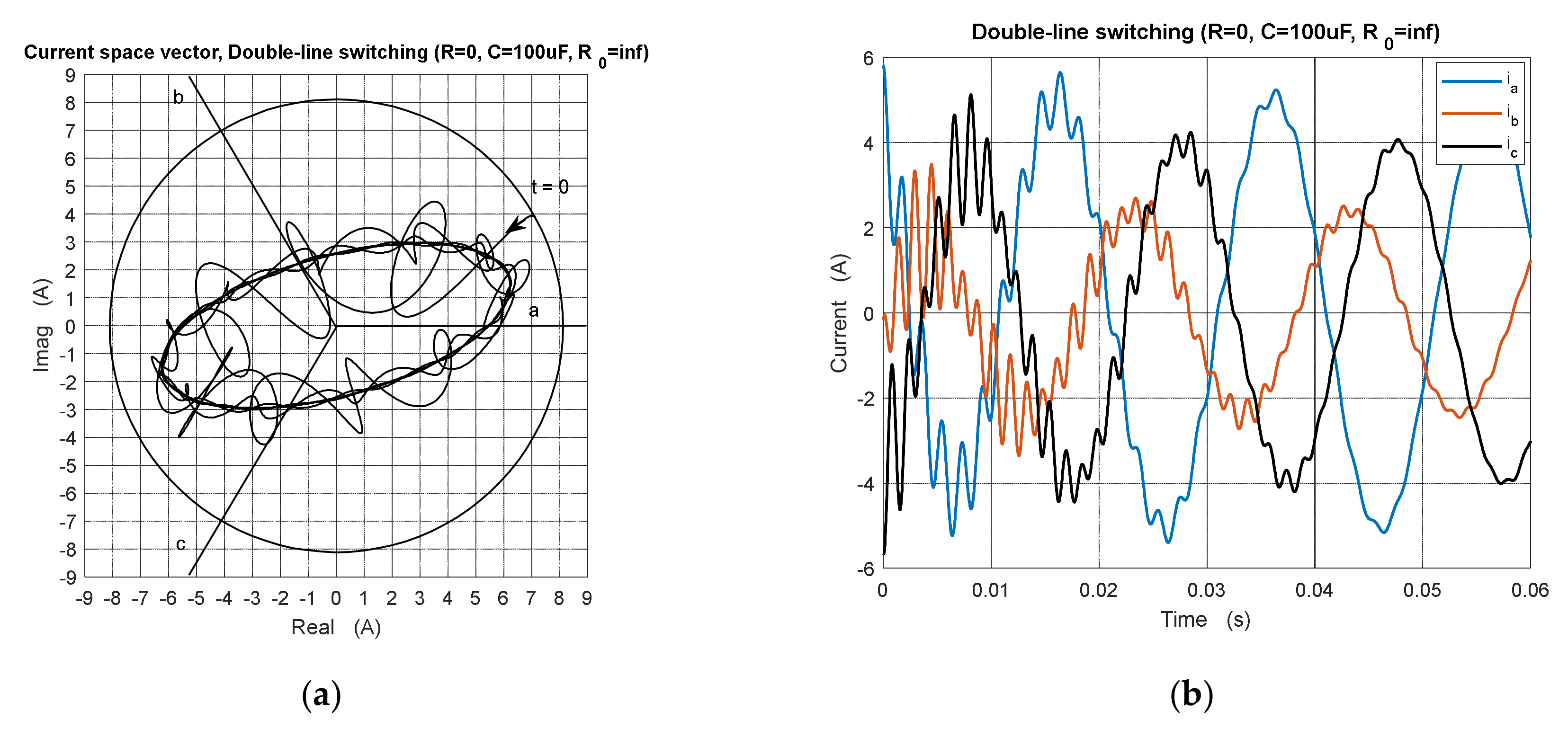
Figure 15a,b shows the results related to the double-line switching, with switch impedance Z consisting only of a capacitor $C=100 \mathsf{\mu }\mathrm{F}$, and an open single-phase circuit (i.e., $R_0\to \infty$). From the circuit models in Figure 7, we observe that in this case, the β circuit has a transient since it is loaded by Z. Therefore, the whole transient is split in two uncoupled transients: the α circuit transient (independent from the 0 circuit because it is open in this case), and the β circuit transient. Notice that the two modal circuits have a different load, i.e., $Z/3$ for the α circuit and Z for the β circuit. Thus, the two solutions must be evaluated separately. The consequence of a transient in the β circuit is clearly apparent in Figure 15a where the range of the β component (i.e., the y-coordinate) of the space vector is much smaller than in the steady state (circle). On the contrary, in the single-line switching, the range of the β component remained unchanged (see Figure 11a). Moreover, since the β component also experiences a transient, the oscillations in the space vector have no preferential direction (unlike the horizontal direction in Figure 11a). Thus, in Figure 15a, the oscillations assume a kind of twirled behavior around the elliptical steady state. Such uniform distribution of the high-frequency oscillations can be clearly observed on the phase currents in Figure 15b.

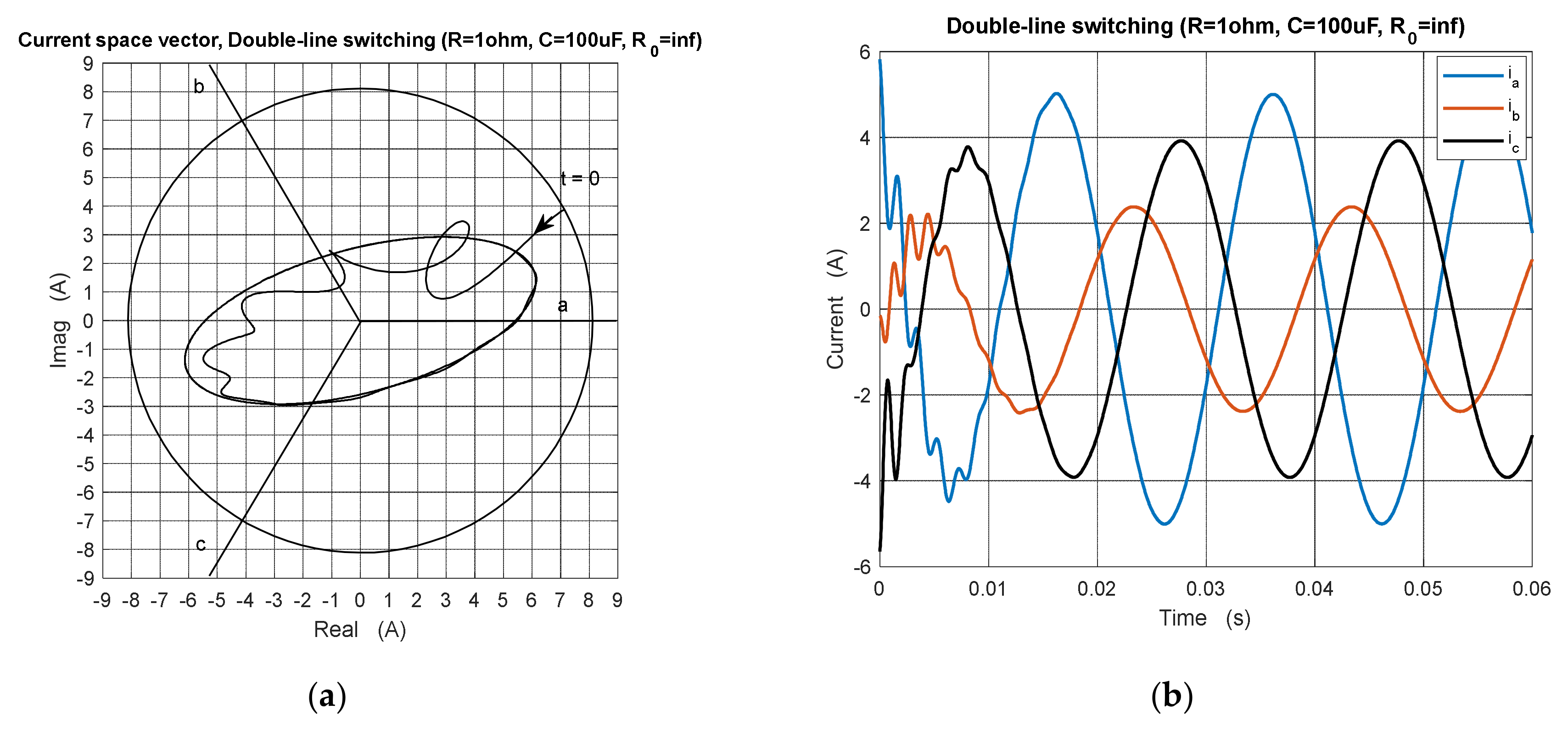
Figure 16a,b shows the effect of a resistor $R=1 \mathsf{\Omega }$ in series with the capacitor $C=100 \mathsf{\mu }\mathrm{F}$ in the line-switch impedance Z. The same damping effect already observed in the single-line case represented in Figure 12a,b is evidenced. The small inclination angle of the ellipse in Figure 16a shows a steady state where the phase current with maximum amplitude is $i_a$ (space vector component on the axis a) and the phase current with minimum amplitude is $i_b$ (space vector component on the axis b). This is confirmed by the time-behavior of the phase currents in Figure 16b.

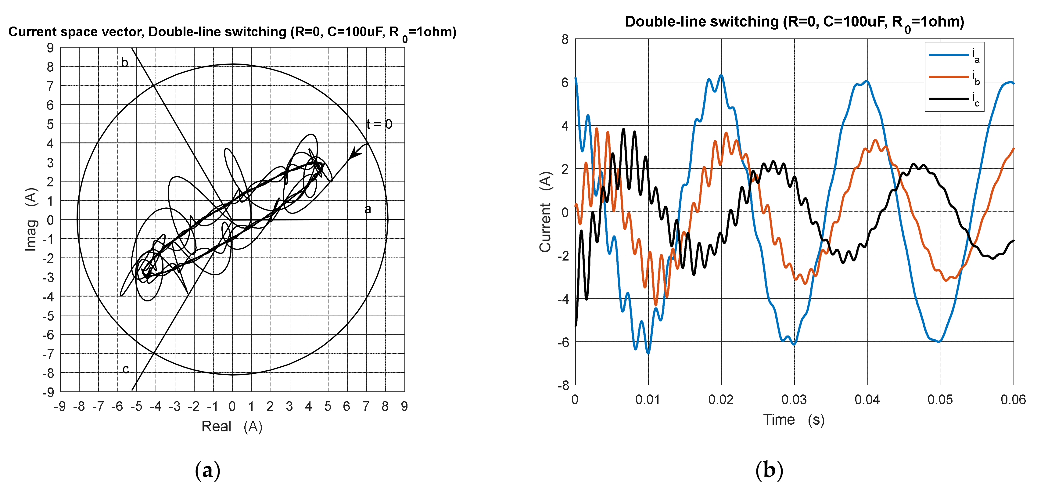
Figure 17a,b shows the effect of the interaction between the 0 circuit and the α circuit (see Figure 7a) due to the single-phase circuit $R_0=1 \mathsf{\Omega }$. The transient of the α circuit is affected by this interaction, whereas the β circuit has an independent transient. This is apparent from the comparison between Figure 15a and Figure 17a. In the two figures, the range of the β component is the same, whereas the dynamics of the α component is different. This results in an ellipse with a smaller range in the α direction. The high-frequency behavior and the steady state in the phase currents are represented in Figure 17b where the relation with the corresponding space vector in Figure 17a can be observed as in the previous cases.

6. Conclusions

The circuit models derived in the paper provide a novel theoretical contribution to the field of asymmetrical three-phase transients which is commonly tackled through numerical approaches. The space vector tool has proven to be very effective in representing in compact form the information about the transient properties.

Future work will be devoted to extending the analysis to the study of a sequence of switching events. This point would be useful to model non-simultaneous operation of the three poles of a breaker, or to model switching events in different sections of a three-phase system.

References

1. Fortescue, C.L. Method of symmetrical coordinates applied to the solution of polyphase networks. Trans. AIEE 1918, 37, 1027–1140. [Google Scholar]
2. Clarke, E. Problems solved by modified symmetrical components. Gen. Electr. Rev. 1938, 41, 488–494. [Google Scholar]
3. Das, J.C. Understanding Symmetrical Components for Power System Modeling; John Wiley & Sons, Inc.: Hoboken, NJ, USA, 2017. [Google Scholar]
4. O’Rourke, C.J.; Qasim, M.M.; Overlin, M.R.; Kirtley, J.L., Jr. A geometric interpretation of reference frames and transformations: dq0, Clarke and Park. IEEE Trans. Energy Convers. 2019, 34, 2070–2083. [Google Scholar] [CrossRef] [Green Version]
5. Paul, C.R. Analysis of Multiconductor Transmission Lines; John Wiley & Sons, Inc.: Hoboken, NJ, USA, 2008. [Google Scholar]
6. Bollen, M.H.J.; Gu, I.Y.H. On the analysis of voltage and current transients in three-phase power systems. IEEE Trans. Power Deliv. 2007, 22, 1194–1201. [Google Scholar] [CrossRef]
7. Mahseredjian, J.; Dinavahi, V.; Martinez, J.A. Simulation tools for electromagnetic transients in power systems: Overview and challenges. IEEE Trans. Power Deliv. 2009, 24, 1657–1669. [Google Scholar] [CrossRef]
8. Van der Sluis, L. Transients in Power Systems; John Wiley & Sons Ltd.: Chichester, UK, 2001. [Google Scholar]
9. Greenwood, A. Electrical Transients in Power Systems, 2nd ed.; Wiley India (P.) Ltd.: New Delhi, India, 1991. [Google Scholar]
10. Owen, M. Transient analysis using component transforms. In Proceedings of the 2011 IEEE Power Engineering and Automation Conference, Wuhan, China, 8–9 September 2011. [Google Scholar]
11. Aller, J.; Bueno, A.; Paga, T. Power system analysis using space vector transformation. IEEE Trans. Power Syst. 2002, 17, 957–965. [Google Scholar] [CrossRef]
12. Ignatova, V.; Granjon, P.; Bacha, S. Space vector method for voltage dips and swells analysis. IEEE Trans. Power Deliv. 2009, 24, 2054–2061. [Google Scholar] [CrossRef] [Green Version]
13. Paap, G.C. Symmetrical components in the time domain and their application to power network calculations. IEEE Trans. Power Syst. 2000, 15, 522–528. [Google Scholar] [CrossRef]
14. Bellan, D.; Superti-Furga, G. Space-vector state-equation analysis of three-phase transients. J. Electr. Syst. 2018, 14, 188–198. [Google Scholar]
15. Bellan, D.; Superti Furga, G.; Pignari, S.A. Circuit representation of load and line asymmetries in three-phase power systems. Int. J. Circuits Syst. Signal Process. 2015, 9, 75–80. [Google Scholar]
16. Bellan, D. Analytical approach to transient solution of single-line and double-line faults in three-phase circuits. Int. J. Circuits Syst. Signal Process. 2019, 13, 647–653. [Google Scholar]
17. Paranavithana, P.; Perera, S.; Koch, R.; Emin, Z. Global voltage unbalance in MV networks due to line asymmetries. IEEE Trans. Power Deliv. 2009, 24, 2353–2360. [Google Scholar] [CrossRef]
18. Dufour, C.; Mahseredjian, J.; Belanger, J. A combined state-space nodal method for the simulation of power system transients. IEEE Trans. Power Deliv. 2011, 26, 928–935. [Google Scholar] [CrossRef]
19. Plumier, F.; Aristidou, P.; Geuzaine, C.; Van Cutsem, T. Co-simulation of electromagnetic transients and phasor models: A relaxation approach. IEEE Trans. Power Deliv. 2016, 31, 2360–2369. [Google Scholar] [CrossRef] [Green Version]
20. Lewis, W.P. Solution of network transients using symmetrical-component techniques. Proc. Inst. Electr. Eng. 1966, 113, 2012–2016. [Google Scholar] [CrossRef]
21. Peralta, J.; De Leon, F.; Mahseredjian, J. Assessment of errors introduced by common assumptions made in power system studies. In Proceedings of the IEEE Power and Energy Society General Meeting, San Diego, CA, USA, 24–28 July 2011. [Google Scholar]
22. Watson, N.R.; Farzanehrafat, A. Three-phase transient state estimation algorithm for distribution systems. IET Gener. Transm. Distrib. 2014, 8, 1656–1666. [Google Scholar] [CrossRef]
23. Kai, T.; Takeuchi, N.; Funabashi, T.; Sasaki, H. A simplified fault currents analysis method considering transient of synchronous machine. IEEE Trans. Energy Convers. 1997, 12, 225–231. [Google Scholar] [CrossRef]
24. Bo, Z.; Weller, G.; Lomas, T. A new technique for transformer protection based on transient detection. IEEE Trans. Power Deliv. 2000, 15, 870–875. [Google Scholar]
25. Wang, X.; Zhang, H.; Shi, F.; Wu, Q.; Terzija, V.; Xie, W.; Fang, C. Location of single phase to ground faults in distribution networks based on synchronous transients energy analysis. IEEE Trans. Smart Grid 2010, 11, 774–785. [Google Scholar] [CrossRef] [Green Version]
26. Cui, T.; Dong, X.; Bo, Z.; Juszczyk, A. Hilbert-transform-based transient/intermittent Earth fault detection in noneffectively grounded distribution systems. IEEE Trans. Power Deliv. 2011, 26, 143–151. [Google Scholar] [CrossRef]
27. Mardiana, R.; Motairy, H.A.; Su, C.Q. Ground fault location on a transmission line using high-frequency transient voltages. IEEE Trans. Power Deliv. 2011, 26, 1298–1299. [Google Scholar] [CrossRef]
28. Ahmadimanesh, A.; Shahrtash, S.M. Transient-based fault-location method for multiterminal lines employing S-transform. IEEE Trans. Power Deliv. 2013, 28, 1373–1380. [Google Scholar] [CrossRef]
29. Satpathi, K.; Yeap, Y.M.; Ukil, A.; Geddada, N. Short-time fourier transform based transient analysis of VSC interfaced point-to-point DC system. IEEE Trans. Ind. Electron. 2018, 65, 4080–4091. [Google Scholar] [CrossRef]
30. Sadeghkhani, I.; Hamedani Golshan, M.E.; Mehrizi-Sani, A.; Guerrero, J.M.; Ketabi, A. Transient Monitoring Function–Based Fault Detection for Inverter-Interfaced Microgrids. IEEE Trans. Smart Grid 2018, 9, 2097–2107. [Google Scholar] [CrossRef] [Green Version]
31. Martins, L.S.; Martins, J.F.; Pires, V.F.; Alegria, C.M. The application of neural networks and Clarke-Concordia transformation in fault location on distribution power systems. In Proceedings of the IEEE/PES Transmission and Distribution Conference and Exhibition, Yokohama, Japan, 6–10 October 2005; pp. 2091–2095. [Google Scholar]
32. Zin, A.A.M.; Saini, M.; Mustafa, M.W.; Sultan, A.R. New algorithm for detection and fault classification on parallel transmission line using DWT and BPNN based on Clarke’s transformation. Neurocomputing 2015, 168, 983–993. [Google Scholar]
33. Bellan, D.; Pignari, S.A.; Superti-Furga, G. Consistent circuit technique for zero-sequence currents evaluation in interconnected single/three-phase power networks. J. Electr. Syst. 2016, 12, 230–238. [Google Scholar]
Figure 1. The phase variables a, b, c can be recovered as the instantaneous components of the space vector on the three axes a, b, and c whose angular displacement on the complex plane is 2 π / 3 .
Energies 13 05231 g001
Figure 2. A generic three-phase circuit including a single-phase circuit connected to the star centers. The three-phase port S is where asymmetrical line switching is operated.
Energies 13 05231 g002
Figure 3. No-load three-phase circuit in the Laplace domain once the asymmetrical three-phase port S is removed.
Energies 13 05231 g003
Figure 4. Laplace-domain Thevenin equivalents of the three modal circuits α, β, 0, according to the Clarke transformation.
Energies 13 05231 g004
Figure 5. Circuit models for the single-line (a) and the double-line (b) switching. When t = 0, the ideal switches open, and the impedances Z are series connected to the corresponding lines.
Energies 13 05231 g005
Figure 6. Connection of Thevenin modal circuits in the Laplace domain. Line switching of phase a result in (a) coupled α and 0 circuits through an ideal transformer with ratio k 1 = 2 and (b) an uncoupled and shorted steady-state circuit β.
Energies 13 05231 g006
Figure 7. Connection of Thevenin modal circuits in the Laplace domain. Line switching of phases b and c results in (a) coupled α and 0 circuits through an ideal transformer with ratio k 2 = 1 / 2 , and (b) an uncoupled circuit β.
Energies 13 05231 g007
Figure 8. Connection of modal circuits in the time domain. Line switching of phases b and c results in (a) coupled α and 0 circuits through an ideal transformer with ratio k 1 = 2 , and (b) an uncoupled and shorted steady-state circuit β.
Energies 13 05231 g008
Figure 9. Connection of modal circuits in the time domain. Line switching of phases b and c results in (a) coupled α and 0 circuits through an ideal transformer with ratio k 2 = 1 / 2 and (b) an uncoupled circuit β.
Energies 13 05231 g009
Figure 10. The three-phase circuit used for simulation analysis of the circuit models derived in the paper. The three-phase port S operates the line switching.
Energies 13 05231 g010
Figure 11. Single-line switching of phase a. Time-behavior of the current space vector (a) and the related phase currents (b) for the three-phase circuit in Figure 10 where S operates single-line switching of phase a with an impedance Z consisting in a capacitor C = 100   μ F . The single-phase circuit is open since R 0 .
Energies 13 05231 g011
Figure 12. Single-line switching of phase a. Time-behavior of the current space vector (a) and the related phase currents (b) for the three-phase circuit in Figure 10 where S operates single-line switching of phase a with an impedance Z consisting of a capacitor C = 100   μ F in series with a resistor R = 1   Ω . The single-phase circuit is open since R 0 .
Energies 13 05231 g012
Figure 13. Single-line switching of phase a. Time-behavior of the current space vector (a) and the related phase currents (b) for the three-phase circuit in Figure 10 where S operates single-line switching of phase a with an impedance Z consisting of a capacitor C = 500   μ F . The single-phase circuit is open since R 0 .
Energies 13 05231 g013
Figure 14. Single-line switching of phase a. Time-behavior of the current space vector (a) and the related phase currents (b) for the three-phase circuit in Figure 10 where S operates single-line switching of phase a with an impedance Z consisting of a capacitor C = 100   μ F . The single-phase circuit consists in R 0 = 1   Ω .
Energies 13 05231 g014
Figure 15. Double-line switching. Time-behavior of the current space vector (a) and the related phase currents (b) for the three-phase circuit in Figure 10 where S operates double-line switching of phases b and c with an impedance Z consisting of a capacitor C = 100   μ F . The single-phase circuit is open since R 0 .
Energies 13 05231 g015
Figure 16. Double-line switching. Time-behavior of the current space vector (a) and the related phase currents (b) for the three-phase circuit in Figure 10 where S operates double-line switching of phases b and c with an impedance Z consisting of the series connection of a capacitor C = 100   μ F and a resistor R = 1   Ω . The single-phase circuit is open since R 0 .
Energies 13 05231 g016
Figure 17. Double-line switching. Time-behavior of the current space vector (a) and the related phase currents (b) for the three-phase circuit in Figure 10 where S operates double-line switching of phases b and c with an impedance Z consisting of a capacitor C = 100   μ F . The single-phase circuit consists in R 0 = 1   Ω .
Energies 13 05231 g017