Thermal Distortion of Signal Propagation Modes Due to Dynamic Loading in Medium-Voltage Cables

Abstract

Temperature variation from dynamic cable loading affects the propagation characteristics of transient signals. The distortion of modal signal components as a function of temperature in a three-phase medium-voltage cable is investigated. The temperature influence arises mainly through the complex insulation permittivity, which has a non-linear relationship with temperature. Near the maximum operating temperature of the cross-linked polyethylene insulation, the propagation velocity increases by 0.56% per degree centigrade but is an order of magnitude less sensitive at ambient temperature. The paper presents modeling results based on cable impedance and admittance matrices obtained from electromagnetic field simulation, taking into account the time-varying temperature distribution in the cable cross-section. The results are verified by applying Rayleigh–Schrödinger perturbation analysis. In the time domain, signal patterns shift when the modal propagation velocities change upon cable loading. Moreover, separation of degenerate modes is observed when the cable phase conductors carry an unbalanced current. The perspectives for exploiting the temperature dependency of signal propagation for pinpointing cable defects and for dynamic rating of underground power cables are discussed.

1. Introduction

Defects in underground power cables can be a source of partial discharges. Partial discharge (PD) signals travel from their origin to the cable ends, where detection takes place. From known propagation characteristics, the location can be determined and the severity of the defect can be assessed [1]. In addition, short faults are observed in live grids both in low-voltage and medium-voltage cables [1,2]. These events concern transient short circuits, typically lasting for a fraction of a power cycle, which is too short to directly cause a system outage. However, these events may act as a precursor for an upcoming failure. In both examples, pinpointing the fault location requires accurate knowledge of the propagation of the transient signals caused by these events.

Propagation characteristics relate to the material properties of the transmission channel. The dielectric permittivity of insulation materials employed in a cable design depends on the temperature, as well as frequency. The consequences for signal velocity can be significant. As an example, Figure 1 illustrates the variation in the propagation velocity along a mass-impregnated cable, which experiences a daily load cycle (mainly during working days). This recording is obtained from online monitoring of a cable connection on PD activity over almost one year. The specific PD system employed here injects a reference pulse every minute to synchronize the detection equipment installed at both cable ends [1]. The figure shows an excerpt of the full recording over four weeks of operation, based on averages over one hour of the measured transit times. The variation is estimated to be around 0.10%/°C [3]. This sensitivity suggests that signal propagation velocity is a feasible indicator of the cable temperature, which can be exploited to optimize the utilization of a cable connection.

A commonly employed insulation material for medium-voltage cables is XLPE (cross-linked polyethylene). The literature on single-phase XLPE cables shows a non-linear increase in the propagation velocity with increasing temperature [4,5,6]. These results are obtained either by time-domain reflectometry (TDR) on a cable section or by analysis of the dielectric material using a vector network analyzer (VNA). As the interests of the authors are related to diagnostic techniques or power line communication, the frequency aimed for is typically in the range of 10 kHz to 10 MHz.

Table 1. Temperature dependency of signal propagation velocity based on time-domain reflectometry (TDR) and permittivity measurement by means of a vector network analyzer (VNA).

Author	Temperature	Change Velocity	Rate of Change	Method
Dubickas et al., 2006 (Table 1 in [4], v~1/√ε’)	20–40 °C 40–60 °C	0.76% 0.92%	0.038 %/°C 0.046 %/°C	TDR and VNA measurement
Li et al., 2015 (estimate from in [5])	25–36 °C 25–45 °C	0.22% 0.90%	0.020 %/°C 0.045 %/°C	TDR and VNA measurement
Nyamupangedengu et al., 2015 1 (abstract of [6])	22–58 °C	4%	0.11 %/°C	TDR measurement

¹ The measured temperature is taken from the earth screen, whereas the phase conductor was inductively heated; the inside cable temperature could have been underestimated.

summarizes the findings of these authors. The relative change in velocity over a given temperature range is provided together with the change per degree centigrade. The literature agrees in the observation that the increased velocity arises from a lowered relative permittivity and that the effect becomes more pronounced at higher temperatures, but it disagrees on the magnitude.

This paper provides a modeling approach to analyze the influence of cable loading on the propagation of modes in a multi-conductor XLPE cable. As a result of the discrepancy in the reported velocity change, the frequency and temperature dependent complex permittivity has been measured. The results of these experiments are presented in Section 2. The modeling approach described in Section 3 consists of modal analyzes, focusing on modified propagation modes in terms of eigenvectors and eigenvalues depending on the temperature distribution. It is applied for both a balanced and an unbalanced cable load. Section 4 analyzes the model results. The implications for the accuracy of defect locating in the case of PD or fault monitoring are discussed. As a second application, the perspective of employing the temperature dependency of signal propagation for dynamic rating of power cables is addressed. The main findings are summarized in Section 5.

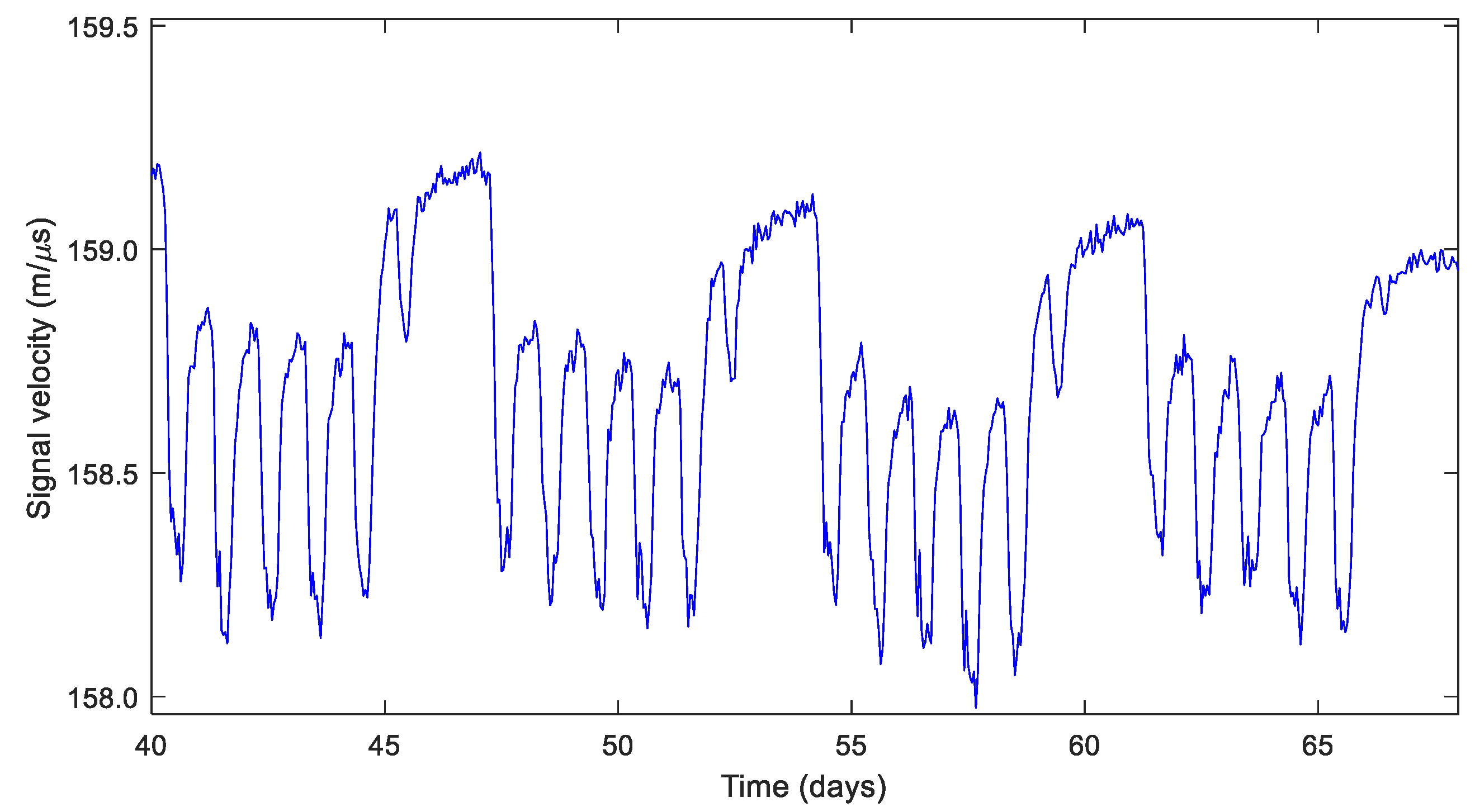
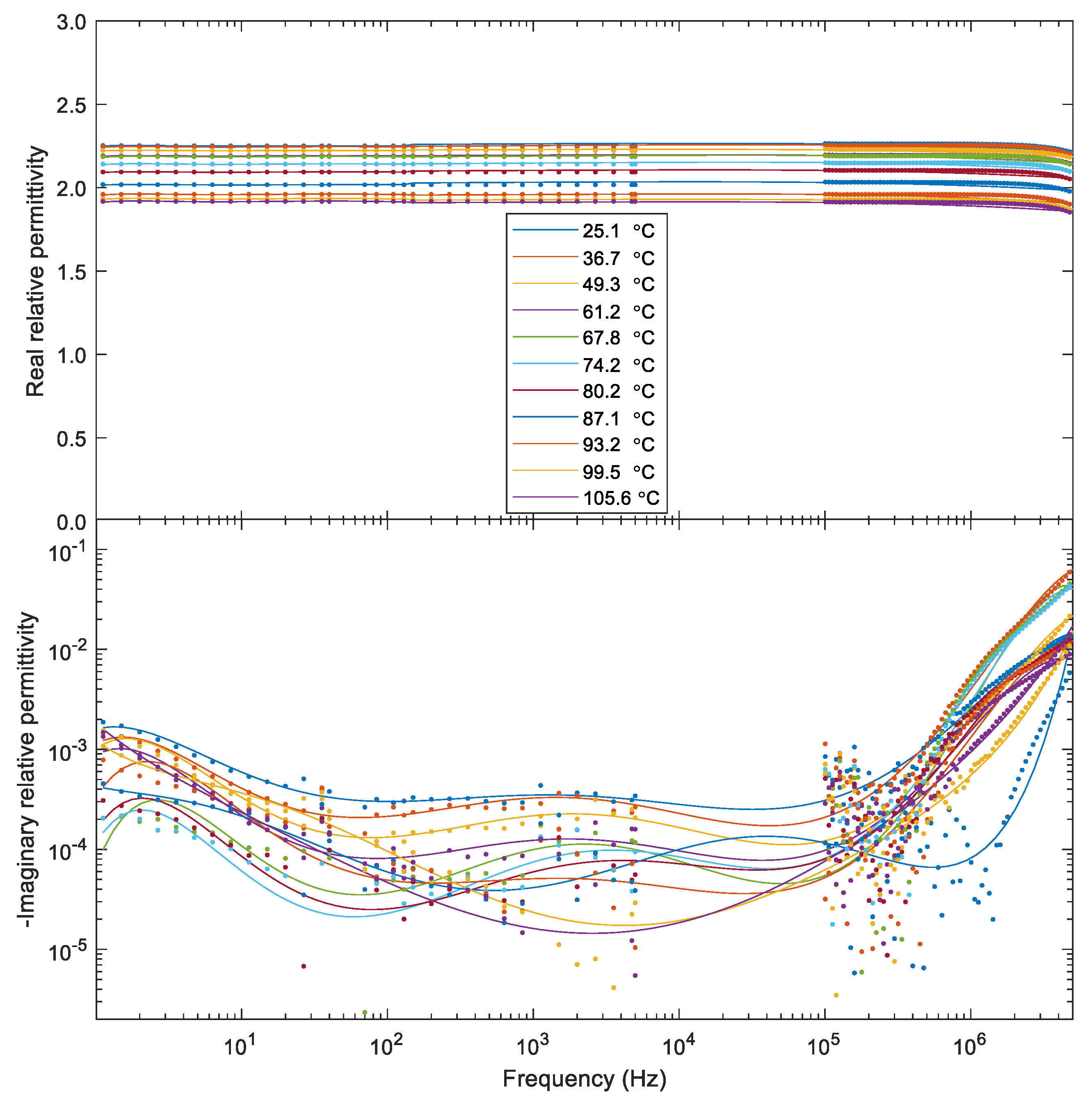
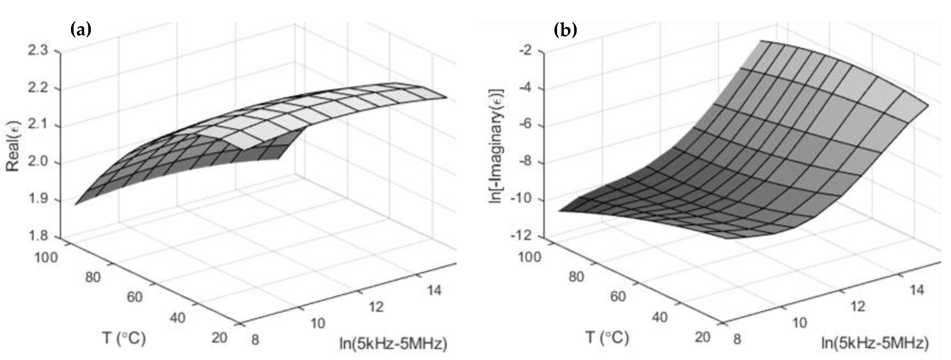
2. Complex Relative Permittivity of XLPE

The permittivity of XLPE is measured over a wide frequency range with dedicated equipment from [7].

• For frequencies up to 5 kHz, a dielectric material analyzer is employed (Spectano 100, test amplitude 200 V)
• A VNA is used for the higher frequency range, up to 5 MHz (Bode 100, test voltage 1 V_rms).
• The upper frequency is restricted by the dielectric sample holder design (DSH 100, temperature up to 125 °C).

The sample holder is thermally insulated by a custom-made box from polyisocyanurate and the temperature is controlled within 0.1 °C. An XLPE sample was prepared with thickness of 1.22 mm (variation of ± 0.02 mm). The electrode diameter (within the guarding electrode) was 5.00 cm.

The relative permittivity is determined by comparing the frequency response of the XLPE sample to the response from an air gap with equivalent dimensions. Such calibration is part of the dielectric material analyzer’s operating procedure but needs to be implemented for the VNA. The measured response represents a first-order high-pass filter. The sample corresponds to its capacitance, which is terminated with resistance R₀ = 50 Ω. The transfer function with the sample can be expressed in terms of the equivalent air capacitance C₀ and the complex relative permittivity ε’ − jε’’:

$$H\left(\omega \right)=\frac{R_0}{R_0+1/\mathrm{j}\omega C_0\left({\epsilon }^{\prime }-\mathrm{j}{\epsilon }^{″}\right)}$$

(1)

Dividing this response by the response H₀ from the air gap (relative permittivity 1) gives

$$\frac{H}{H_0}\left(\omega \right)=\frac{1+\mathrm{j}\omega R_0{C}_0}{\frac{1}{\left({\epsilon }^{\prime }-\mathrm{j}{\epsilon }^{″}\right)}+\mathrm{j}\omega R_0{C}_0}$$

(2)

The complex relative permittivity can therefore be expressed in terms of the transfer function ratio of measurements with the XLPE sample and with an equivalent air gap:

$${\epsilon }^{\prime }\left(\omega \right)-\mathrm{j}{\epsilon }^{″}\left(\omega \right)=\frac{H}{H_0}{\left[1+\mathrm{j}\omega R_0{C}_0\left(1-\frac{H}{H_0}\right)\right]}^{-1}$$

(3)

The value for the air capacitance is taken from the dielectric material analyzer calibration, C₀ = 14.25 pF. The absolute value of the second term between square brackets in (3) at the maximum frequency of 5 MHz is relatively small (around 2% of the first term). This means that the real permittivity is equal to the ratio of the transfer functions with a small correction. The reported dielectric losses of XLPE in the literature are low, with a typical value of −0.001 j for the imaginary permittivity [8]. This challenges its accurate determination. The imaginary part of the transfer function ratio is small compared to the real part and the aforementioned correction in (3) compensates with a value of almost the same magnitude. This can cause relatively large uncertainty.

Figure 2 shows the real and imaginary permittivity over a frequency range from 1 Hz to 5 MHz. The real part is constant with frequency. A small correction of 2% was made on the VNA dataset for the real permittivity to match more precisely the real permittivity values from the dielectric material analyzer data [3]. Such differences can arise due to instrument tolerance. Moreover, the dielectric material analyzer software corrects for fringing electric fields at the sample edges. The sample temperature is varied from ambient to just over 100 °C. The decrease in the real permittivity with temperature as observed in [4,5] is confirmed, including its non-linearity. Near ambient temperature, the change is relatively small, measuring −0.068 %/°C (mean difference over measurements at 25.1 and 36.7 °C). The signal velocity scales inversely with the square root of the relative permittivity, resulting in a value of 0.034 %/°C, agreeing closely with [4]; see Table 1. The relative permittivity change is largest near 90 °C (maximum operating temperature for XLPE), with −1.12 %/°C, corresponding to a velocity variation of 0.56 %/°C.

The imaginary part is hard to determine accurately and exhibits a large spread, particularly for the VNA measurements. The solid lines in Figure 2 are polynomial fits, meant as a “guide to the eye”. The losses increase beyond 0.1–1 MHz and may add to the signal attenuation caused by conductor losses and losses related to the semiconductive material [9,10]. For signal propagation analysis, the response in the higher frequency range is most relevant. Therefore, the data below 5 kHz will be discarded from further analysis.

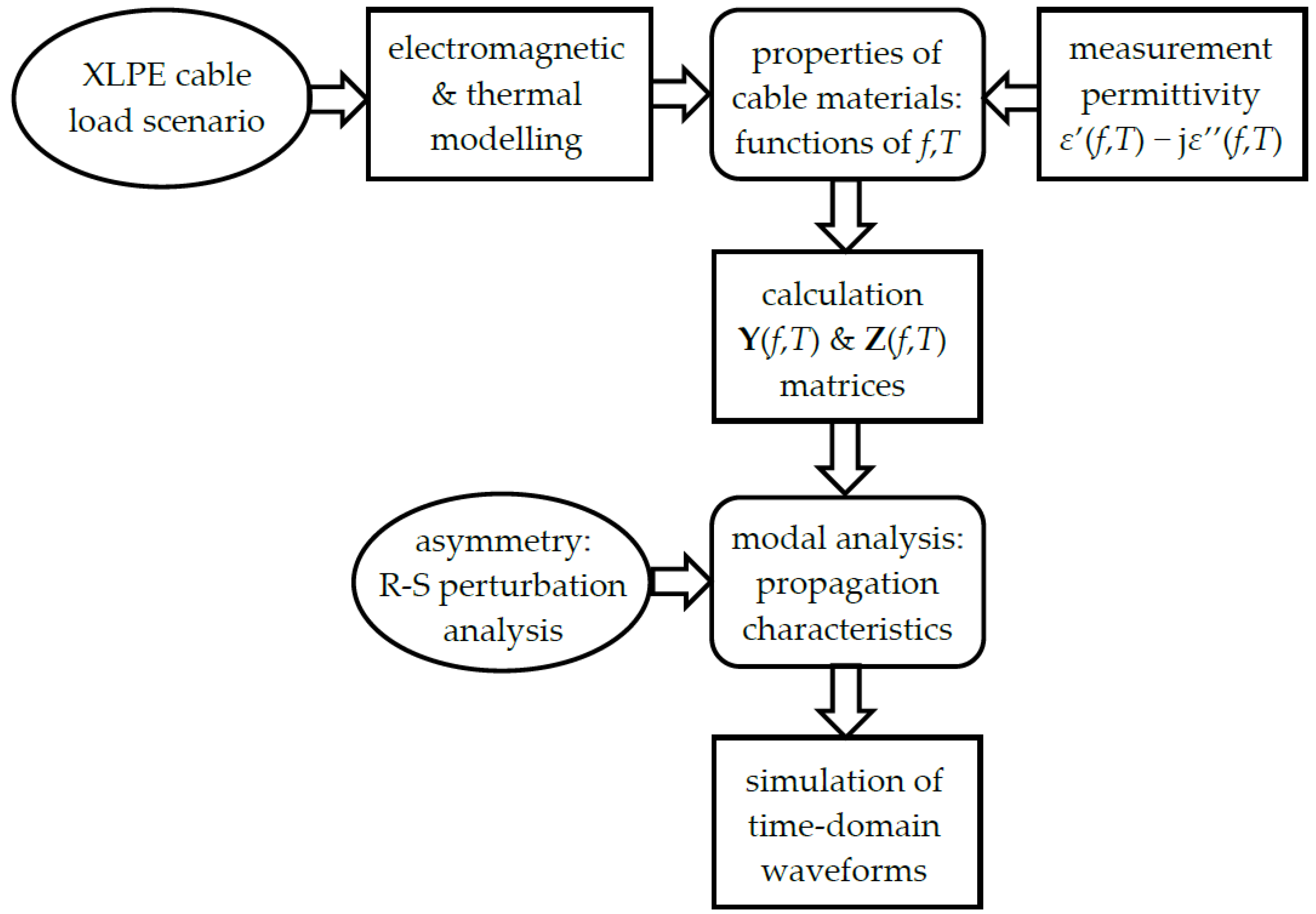
3. Propagation Mode Modeling

The scheme to model the signal propagation along a multi-core XLPE-insulated cable is depicted in Figure 3. First, for a defined load applied to the cable, the electromagnetic field distribution is determined. This information is used to calculate the heat dissipation needed for thermal modeling. Next, the temperature distribution is converted to a distribution of the complex permittivity throughout the cable cross-section. The temperature and frequency dependent permittivity affects the admittance matrix Y. The impedance matrix Z is temperature dependent through the conductor resistivity. Frequency dependency arises from skin and proximity effect. From the matrices, the eigenmodes with their propagation coefficients are calculated. The modes have a simple structure for three-fold rotation-symmetric cables with balanced loading. For unbalanced phase currents, the modes are distorted. The eigenmodes become frequency dependent but can still be related to the original symmetric modes, e.g., through Rayleigh–Schrödinger (R–S) perturbation analysis [11]. Finally, the time-domain responses are evaluated upon an injected pulse.

The cable design is depicted in

Table 2. Dimensions of a three-phase medium-voltage XLPE cable.

Parameter	Value
radius aluminum conductors, r1	8.55 mm
radius conductor screens, r2	9.35 mm
radius XLPE insulation layers, r3	12.75 mm
radius insulation screens, r4	14.00 mm
distance conductors to center, dk	16.16 mm
radius filler material, rp1	30.15 mm
radius swelling tape, rp2	30.50 mm
radius copper earth screen, rp3	31.50 mm
outer radius cable jacket, rp4	33.00 mm

. It consists of three aluminum phase conductors and a common copper earth screen. Semiconductive screens are located at the inside and outside of the XLPE insulation and a swelling tape is applied at the inside of the earth screen. The space in between contains a filler material and a jacket surrounds the assembly.

3.1. Electromagnetic and Thermal Modeling

The conductor resistivity is temperature dependent. This implies the need for a multi-physics approach. Skin and proximity effects determine the current distribution in the conductors, which causes the heat generation. As temperature rises, the conductor resistivity changes, which in turn affects the current distribution. The semiconductive layers and swelling tape are integrated with the insulation material in this modeling stage, since these layers are relatively thin and are expected to have similar thermal properties as XLPE and filler material. The heat loss from the cable to the environment is modeled by means of a soil layer with a one meter radius with constant ambient temperature outside. In reality, the soil temperature dynamics are complex because the heat transfer to the soil depends on the load history and also on thermal variations in the local environment [12].

The thermal response simulated with Comsol Multiphysics [13] is shown in Figure 4. The relevant material parameters are summarized in

Table 3. Electrical and thermal properties; brackets indicate no relevance for the simulations.

Material Property 1	Aluminum	Copper	XLPE	Filler	Jacket	Soil
electric resistivity in Ω·m	2.65 × 10−8	1.72 × 10−8	(∞)	(∞)	(∞)	(100)
at reference temperature	20 °C	25 °C
relative permittivity	1	1	Figure 5	4	(4)	(10)
specific heat capacity in J/kg·K	900	385	2581	1700	1000	1470
thermal conductivity in W/m·K	238	400	0.29	0.26	0.19	1
density in kg/m3	2700	8960	930	1150	1300	1300

¹ Semiconductive layers and swelling tape are omitted from thermal modeling; for analysis of the propagation coefficient, relative permittivity is 1000, resistivity is 0.033 Ω·m and 0.010 Ω·m, respectively.

. The current applied to the cable is taken 1¾ times and 1¼ times the nominal value (nominal current: 360 A). Similar conductor temperatures are reached at the end of both simulations, i.e., after 1¾ hours and 75 h, respectively. Although the final conductor temperatures are similar, there is a significant difference of 14 °C in the temperatures of the earth screen. Rapid heating results in a large temperature gradient in the cable cross-section. The simulation suggests that signal propagation is expected not to be solely determined by the conductor temperature. It also depends on the loading scenario by which the temperature is reached.

3.2. Modeling Material Properties

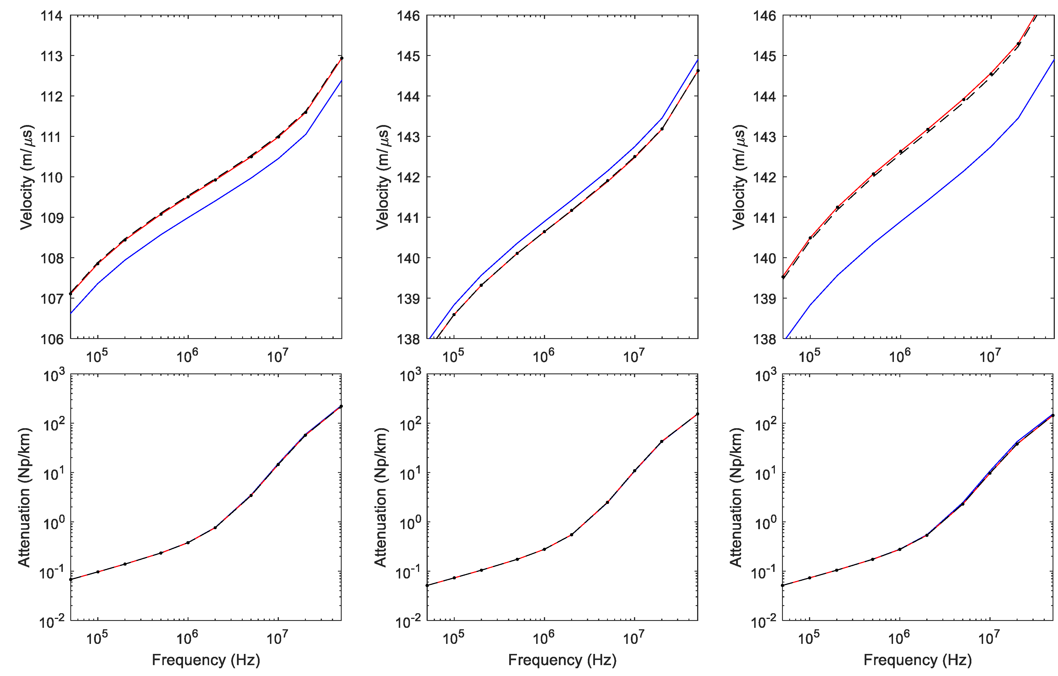
For the simulation of the propagation characteristics, the impedance and admittance matrices are determined. The former are calculated through a magnetic field solver (Oersted [14]) and the latter through an electric field solver (Electro [14]). As input, the temperature dependent conductor resistivity and the insulation permittivity distribution need to be supplied, respectively.

For the resistivity ρ, a linearized temperature dependency is used:

$$\rho \left(T\right)={\rho }_0\left[1+\alpha \left(T-T_0\right)\right]$$

(4)

The resistivity ρ₀ at reference temperature T₀ is provided in Table 3. A resistivity temperature coefficient α = 0.0039 °C⁻¹ is taken for both the aluminum conductors and the copper earth screen.

The complex permittivity is based on the experimental data presented in Section 2. The temperature dependency is only relevant for the XLPE layers since the electric field is confined by the semiconductive layers. Each XLPE layer is divided into smaller segments, and, for each, the average temperature from the thermal simulation is taken. The corresponding permittivity is based on the data in Figure 2. A two-dimensional polynomial fit is made as a function of ln(f), with frequency f ranging from 5 kHz to 5 MHz, and temperature T. The fitted relationships for ε’(ln(f),T) and ln(ε’’(ln(f),T)) shown in Figure 5 enable interpolation of the complex permittivity and suppress the scatter in the data. The fit parameters are provided in Appendix A.

3.3. Modal Analysis

Medium-voltage power cables can be realized with three rotationally symmetric positioned phase conductors enclosed by a common earth screen. Modal analysis of such multi-conductor transmission lines is treated in several textbooks, e.g., [15,16,17]. The phase voltages in the frequency domain as a function of the cable position z can be expressed in terms of the cable impedance matrix Z and admittance matrix Y:

$$\frac{{\partial }^2}{\partial z^2}\mathit{U}\left(z\right)=\left(ZY\right)\mathit{U}\left(z\right)$$

(5)

The impedance matrix includes per-unit-length series inductances and resistances. Per-unit-length shunt capacitances and conductances are accounted for by the admittance matrix. Modal voltages are obtained by finding the eigenvectors and eigenvalues of the product ZY.

The cable geometry shown next to Table 2 has a three-fold rotational symmetry as well as reflection symmetry with respect to a line through the cable center and a phase conductor. This will be reflected in the structure of the ZY matrix if the cable material properties exhibit similar symmetry. When all conductors carry equal currents and the thermal losses to the environment are homogeneous, the temperature distribution will obey the same symmetry. Such a ZY matrix is referred to as “circulant” [18,19] and the eigenvectors take a simple form [11]:

$$\left(\begin{array}{c}⅓\sqrt{3}\\ ⅓\sqrt{3}\\ ⅓\sqrt{3}\end{array}\right) , \left(\begin{array}{c}½\sqrt{2}\\ 0\\ -½\sqrt{2}\end{array}\right) , \left(\begin{array}{c}⅙\sqrt{6}\\ -⅓\sqrt{6}\\ ⅙\sqrt{6}\end{array}\right)$$

(6)

The first eigenvector is nondegenerate, whereas the second and third eigenvector belong to the same eigenvalue. The degenerate eigenvectors are chosen to be orthogonal, and all vectors are normalized. These vectors are the columns of the transformation matrix T, which relates the phase voltages U to the modal voltages U_m. The eigenvalues provide the modal propagation coefficients γ_m,k and are numerically calculated from the simulated impedance and admittance matrices as functions of frequency and temperature:

$$\begin{array}{c}{\mathit{U}}_m\left(z\right)=T^{-1}\mathit{U}\left(z\right)={\mathrm{e}}^{-{\gamma }_{m}z}{\mathit{U}}_m\left(0\right)\\ {\gamma }_{m,k}={\alpha }_k+\mathrm{j}{\beta }_k \mathrm{and} v_k=\frac{{\beta }_k}{2\mathsf{\pi }f}\end{array}$$

(7)

The diagonal matrix γ_m contains the modal propagation coefficients as diagonal elements, which are the square roots of the eigenvalues of matrix ZY. The real part of each mode k provides the signal attenuation coefficient α_k and the phase velocity v_k is found from the imaginary part, the phase coefficient β_k.

With an unbalanced load, the symmetry is broken and the modes in (6) are distorted. The overall change in the real permittivity observed from Figure 2 is around 10%. This implies that the propagation velocity varies by around 5%. One can expect that the distortion in eigenvectors and eigenvalues is small as well. However, the originally degenerate mode will become nondegenerate. Which linear combination of the degenerate modes in (6) will match the distorted system depends on the kind of perturbation. Numerical analysis of the perturbed ZY matrix will provide the correct eigenvalues and eigenvectors. The latter will become complex, with frequency dependent components upon asymmetry. An alternative approach is to apply Rayleigh–Schrödinger perturbation analysis [20,21]. The deviation due to the unbalanced current distribution with respect to a balanced one, in terms of the ZY product, is determined. This difference is considered as a perturbation term from which a correction of the corresponding eigenvalues can be calculated [11]. It informs whether the original eigenvectors are still good representations of the perturbed modes.

A simulation example is depicted in Figure 6. It corresponds to the thermal distribution reached after three hours, starting from 15 °C, with 1.8 times the nominal current. This (unusual) condition is taken to enforce a relatively large temperature gradient throughout the cable cross-section to demonstrate the effect on the propagation coefficients. Details of the simulation are provided in Appendix B. Propagation velocity and attenuation are depicted as functions of frequency, which are ordered according to the corresponding eigenvectors in (6). For a balanced load (blue curves), the phase velocity of the first mode is significantly lower, with slightly increased attenuation compared to the others. Unbalance is added by an increased current of 20% in one phase, while the others are reduced with 10%. From the analysis of the corresponding ZY matrices (red curves), it is observed that the velocities of the degenerate modes diverge by around 1.4%. Results of Rayleigh–Schrödinger perturbation analysis indicate that the distorted modes can still be interpreted in terms of the original ones valid for perfect symmetry. First-order perturbation results (dashed curves) match closely already. With second-order perturbation (dotted curves), equal results are obtained as from directly evaluating the ZY matrices. Appendix B shows that the eigenvector elements remain close to the ones in (6).

The average temperature of the insulation around the phase carrying the largest current was around 95 °C. The average insulation temperature near the other phases was 85 °C. Although the temperature difference is only 10 °C, it occurs at the range where the relative permittivity variation is largest.

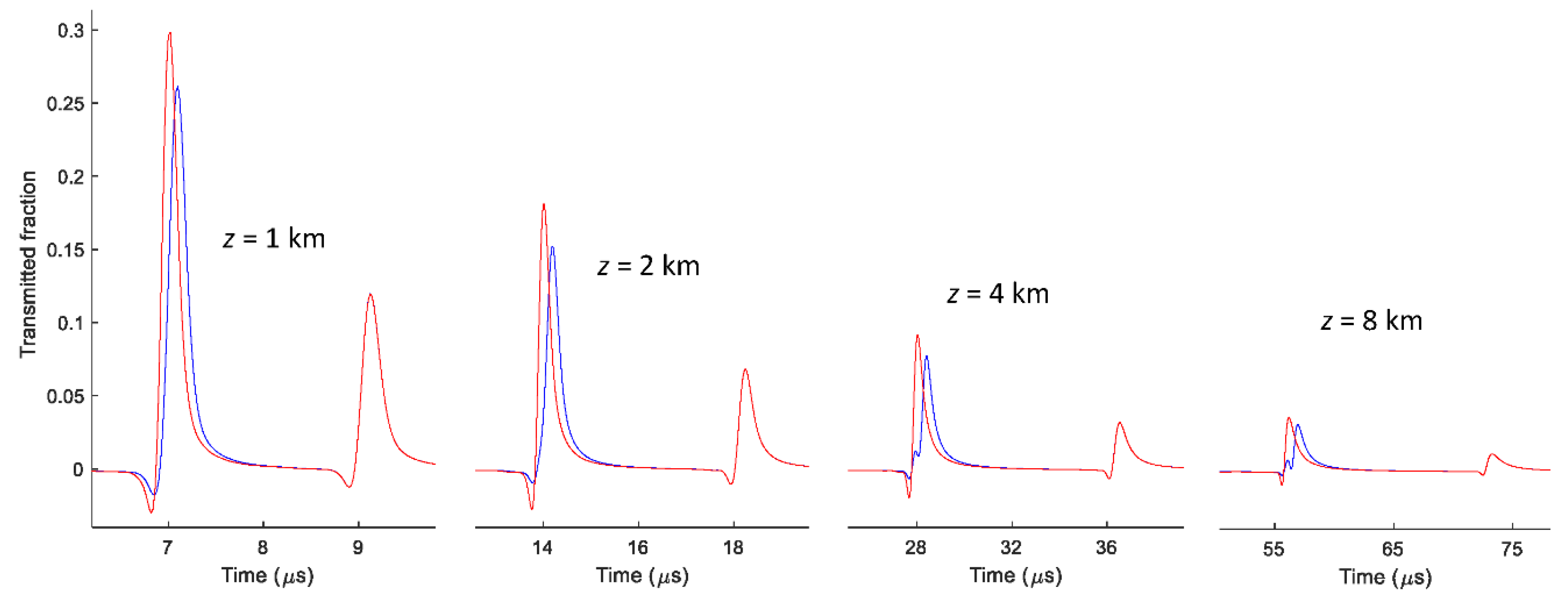
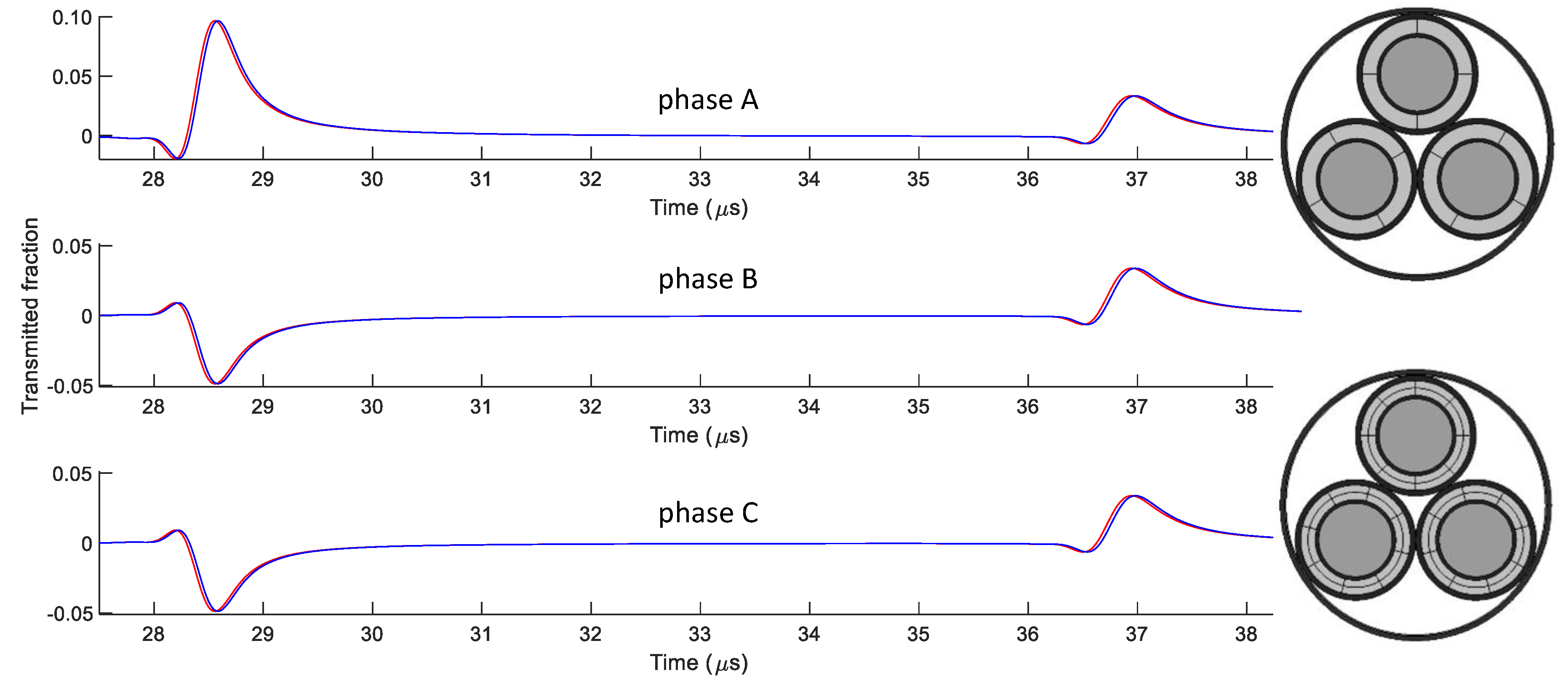
3.4. Time-Domain Response

The time-domain response u(t,z) on an initial signal u(t,0) is calculated in the following sequence:

• The initial signal at z = 0 is converted to the frequency domain by a Fourier transform

  $$\mathit{U}\left(\omega ,0\right)=ℱ\left(\mathit{u}\left(t,0\right)\right)$$
• The frequency-domain signal is decomposed in the modal components

  $${\mathit{U}}_m\left(\omega ,0\right)=T^{-1}\mathit{U}\left(\omega ,0\right)$$
• The modal components after traveling distance z are calculated

  $${\mathit{U}}_m\left(\omega ,z\right)={\mathrm{e}}^{-{\gamma }_m\left(\omega \right)z}{\mathit{U}}_m\left(\omega ,0\right)$$
• The modal components are converted back to phase signals

  $$\mathit{U}\left(\omega ,z\right)=T{\mathit{U}}_m\left(\omega ,z\right)$$
• The phase signals are converted to the time domain with the inverse Fourier transform

  $$\mathit{u}\left(t,z\right)={ℱ}^{-1}\left(\mathit{U}\left(\omega ,z\right)\right)$$

For a narrow pulse (approximated as delta function) applied to a single phase, and applying the eigenvectors of (6) for the transformation matrix T, the response in the frequency domain is

$$\begin{gathered} \mathit{U}\left(\omega ,z\right)={\mathrm{e}}^{-{\gamma }_0\left(\omega \right)z}\left(\begin{array}{c}⅓\\ ⅓\\ ⅓\end{array}\right)+{\mathrm{e}}^{-{\gamma }_{11}\left(\omega \right)z}\left(\begin{array}{c}½\\ 0\\ -½\end{array}\right)+{\mathrm{e}}^{-{\gamma }_{12}\left(\omega \right)z}\left(\begin{array}{c}⅙\\ -⅓\\ ⅙\end{array}\right) \\ =⅓\left(\begin{array}{c}{\mathrm{e}}^{-{\gamma }_0\left(\omega \right)z}+2{\mathrm{e}}^{-{\gamma }_1\left(\omega \right)z}\\ {\mathrm{e}}^{-{\gamma }_0\left(\omega \right)z}-{\mathrm{e}}^{-{\gamma }_1\left(\omega \right)z}\\ {\mathrm{e}}^{-{\gamma }_0\left(\omega \right)z}-{\mathrm{e}}^{-{\gamma }_1\left(\omega \right)z}\end{array}\right) \end{gathered}$$

(8)

Each propagation coefficient contributes to a distinct structure in the time-domain waveforms (γ₀: nondegenerate mode; γ₁₁ and γ₁₂: degenerate modes). With symmetry, the degenerate coefficients are equal (γ₁ ≡ γ₁₁ = γ₁₂) and the modes cannot be distinguished. When introducing asymmetry through unbalanced phase currents, these modes separate.

The aforementioned scheme is applied for the unbalanced current distribution from Section 3.3. Figure 7 demonstrates the signal waveforms for an injected pulse (100 ns wide) either at the phase with the highest temperature (red curves) or at one of the other phases (blue curves). The responses for a TDR measurement on a 0.5, 1.0, 2.0 and 4.0 km cable length (traveled distance is twice this length) are shown. The signals are recorded at the phase conductor with signal injection. The (originally) degenerate modes are around 30% faster than the nondegenerate one according to Figure 6. This agrees with the time difference between the peaks in each waveform. The amplitude ratio complies with the expected relative contributions from the modes according to (8). When injection takes place in the phase with a different temperature compared to the others, reflection symmetry remains. As a consequence, the second mode in (6) is not excited. Both degenerate modes are excited with injection in one of the other phase conductors. These modes deviate slightly upon unbalance because of the 1.4% difference in velocity. This difference becomes visible in peak separation after sufficient traveled distance.

4. Discussion

The sensitivity to material properties and model simplifications are evaluated in Section 4.1. Simulations include the thermal response of a cable after three hours for an overload of 80%. The perspectives on implementing thermal modeling as part of cable condition assessment or dynamic loading are briefly discussed in Section 4.2. The thermal response of a cable for an overload situation of 75% after three hours is compared to the response after several days for nominal current and 25% overload. All simulation conditions correspond to TDR on 2 km cable length and at an initial ambient cable temperature of 15 °C.

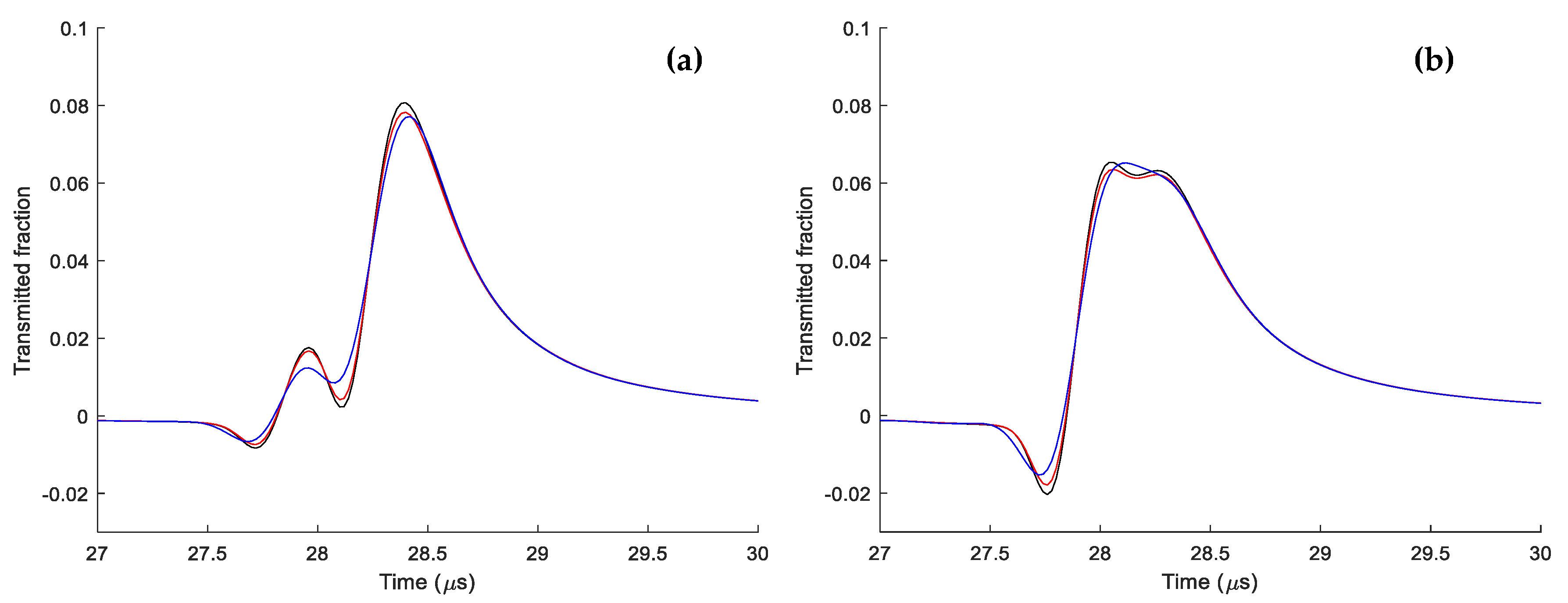
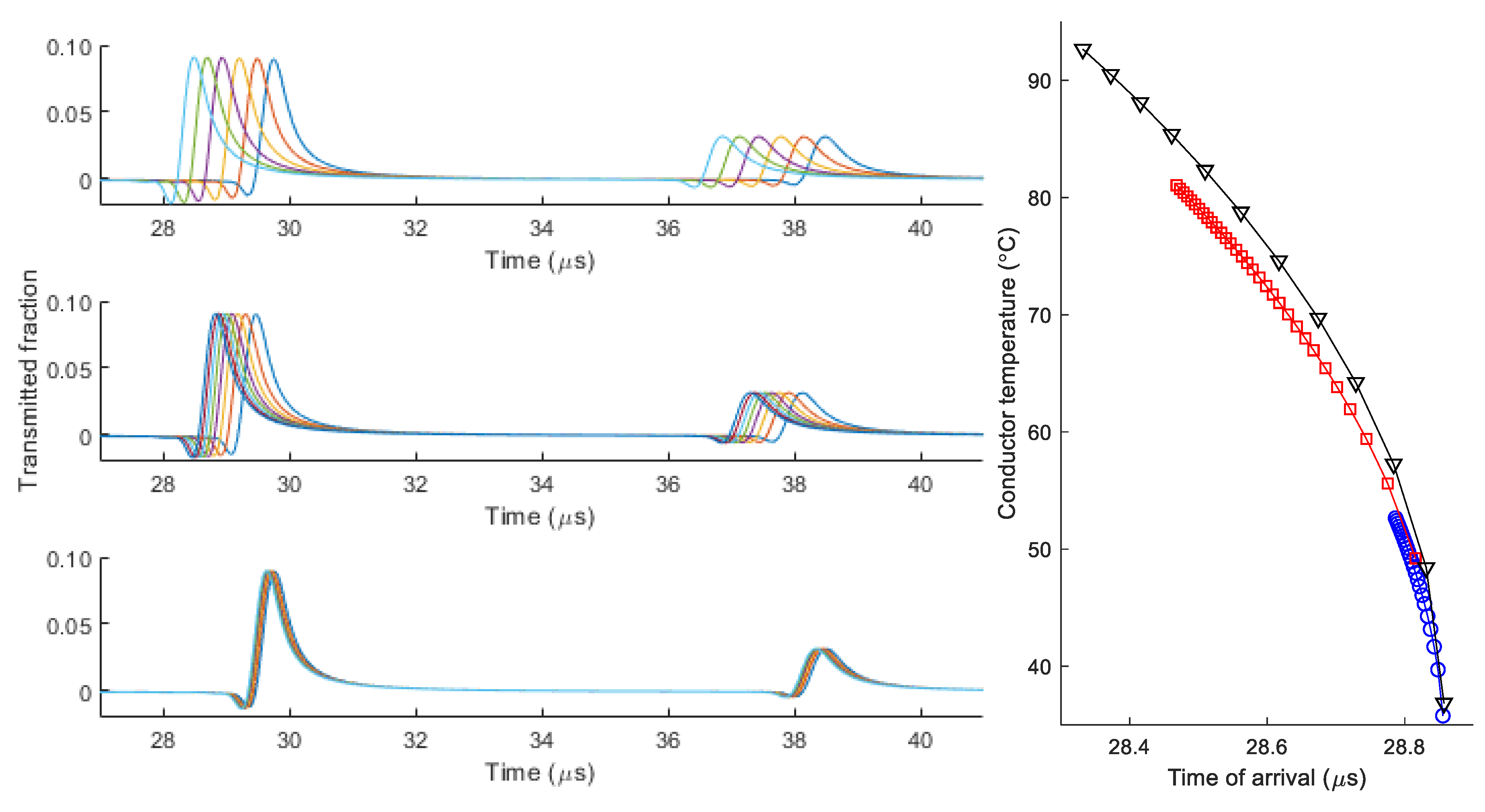
4.1. Sensitivity Analysis

Assumptions and simplifications are unavoidable in the modeling procedure. Thermal analysis is performed without considering the semiconductive layers and swelling tape as part of the insulation. Resistive losses in the conductors are the dominant source of heat dissipation. The time averaged losses over a complete power cycle are used because the temperature hardly varies within this timescale. The dissipation is calculated from the equivalent resistivity of the conductors, which accounts for the skin and proximity effects on the current distribution.

The electric fields are confined to the XLPE layers by the semiconductive layers. Therefore, the temperature dependency of XLPE properties mainly contributes to the shunt admittance. The dielectric permittivity is based on the interpolation of measured values (Appendix A). The dielectric losses are small and could suffer from measurement inaccuracy. Figure 8 shows the effect on the peak arising from the degenerate mode for unbalanced loading. The measured complex permittivity is compared with a fixed complex permittivity of −0.001 j [8] and with no dielectric losses at all. The double peak structure diminishes in Figure 8a, representing the situation in which one phase carries 20% more and the others 10% less than the average current. In Figure 8b, with one phase 20% lower and the others 10% higher current, the double peak vanishes when accounting for the measured dielectric losses. This can be attributed to the steep rising imaginary permittivity, as observed above 1 MHz in Figure 2.

The information passed on from the thermal model (based on the finite element method with [13]) to the pulse propagation modeling (using the boundary element method with [14]) involves average temperature values in defined regions of the cable cross-section. Electric conductors are good thermal conductors, meaning that the temperature across each separate conductor cross-section is close to constant. Electric insulators are thermally insulating as well, which causes a temperature gradient in the insulation. Therefore, each XLPE layer has been divided into four segments (each the size of a quarter of a ring). The electric field is expected to be roughly homogeneous and concentrated in the relatively narrow XLPE layers. Furthermore, the temperature difference and consequently the variation in permittivity are modest. To investigate whether the low number of four XLPE segments is sufficient, each XLPE layer has also been divided into 16 segments (two concentric layers of eight equal segments around the conductor). Figure 9 shows the waveforms observed at the three conductors for a balanced loaded cable. An increased number of XLPE segments causes a systematic but minor shift of around 0.1%. Note that the relative amplitudes of the contributions from the different modes recorded at the three phase conductors agree strongly with the ratios expected from (8).

4.2. Application Perspectives

Defect locating based on traveling waves relies on time of arrival, both when double-sided detection and when TDR from a single end are employed. Signal distortion may diminish the accuracy of either technique. For example, the small peak preceding the larger one in Figure 8a can be below or above a detection threshold level for assigning the time of arrival of the signal. Contributions in the waveforms from similar modes need to be compared. If the sum signal of the three phase conductors is detected (e.g., by having a current probe as sensor enclosing all phase conductors), the contributions from the degenerate modes cancel and only the slower nondegenerate mode is observed. A sensor at a single phase will respond on the first arriving peak in the waveform. This is the degenerate mode for the cable investigated here, which is also detected most easily because of its larger amplitude. The difference in time of arrival is preferably related to the full cable transit time. Such information is available when, in the recorded waveform, patterns are present that have traveled the full cable length. The defect location can then be determined as a fraction of the cable transit time. Otherwise, precise knowledge of the propagation velocity is required.

The change in velocity with temperature is significant mainly at higher temperatures for XLPE. This presents the opportunity to employ propagation characteristics as a source of information for the dynamic rating of medium-voltage cables. For medium-voltage cables, the temperature monitoring functionality is commonly not present as in high-voltage cable connections with optical fibers [22]. Signal propagation analysis can serve as an alternative for monitoring the average temperature of a cable. Contrary to fiber optic techniques, this approach lacks the option to detect local hotspots along a cable connection. An advantage could be that the insulation temperature itself is probed rather than an outer, less heated cable region where a glass fiber is usually situated.

As illustration, Figure 10 compares shifts in recorded signals for three situations with balanced currents.

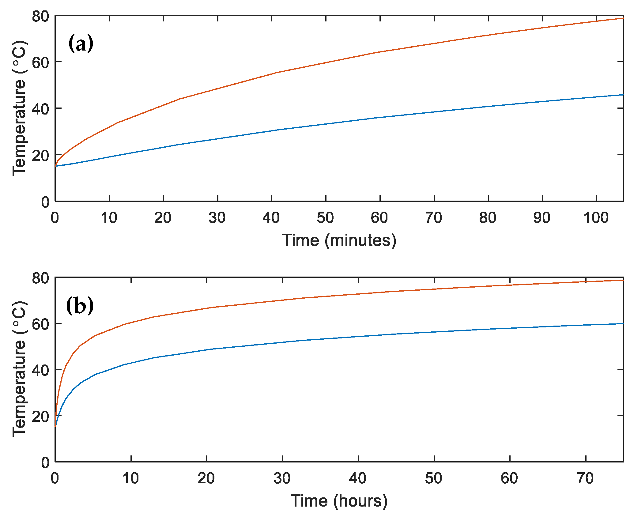
• When the load is 75% higher than nominal, the maximum temperature allowed is reached in three hours. This unrealistic load situation exemplifies the effect of large temperature differences in the cable cross-section.
• A 25% increase over the nominal current is more realistic. Such situations can arise, for instance, in which a parallel connection is temporarily out of service. The current level can be maintained as long as the cable temperature remains within safe operation range.
• For a nominal load, the cable temperature stays within a safe range. The change in the relative permittivity is low, resulting in only minor shifts in the waveform.

The waveforms in Figure 10 show samples taken up to the maximum simulated time every half hour for the first subfigure and every twelve hours for the others. The conductor temperature for the simulations over several days only slightly increases afterwards. The waveforms still shift because of the relatively large change in relative permittivity. The time of arrival, used for the right subfigure in Figure 10, is defined as the moment at which the signal level reaches 10% of its peak value. The conductor temperature is not uniquely determined by the time of arrival. A higher load causes a larger temperature gradient, meaning a reduced average XLPE temperature compared to the conductor temperature. This is reflected in a lower signal velocity as compared to the other load scenarios. The figure indicates that uncertainty in the measured time of arrival causes inaccuracy in the temperature estimate. The slope of the curve is considerably less when reaching 90 °C, resulting in higher precision compared to near ambient temperatures.

5. Conclusions

Temperature variation affects propagation characteristics in multi-conductor power cables. The dependency arises mainly from the relative permittivity, which, for XLPE, drops with increased temperature. This paper presents a modeling scheme to predict the signal waveforms for dynamical cable load patterns.

Distorted propagation modes in multi-conductor cables upon an inhomogeneous temperature distribution can have adverse effects on condition monitoring techniques that rely on the detection of transient signals traveling along the cable. Each mode has a well-defined velocity. Selection of the contributions of the same mode in the signals from TDR measurements or recordings at both cable ends in the case of two-sided detection improves accuracy.

The change in propagation velocity offers the opportunity to monitor cable temperature through measuring the transit times of injected signals. The temperature distribution not only depends on the momentary temperature but is also affected by the load history. Therefore, accurate temperature monitoring also involves thermal modeling based on logged load currents. Such modeling can be delicate, because the heat transfer to the environment depends on the soil properties, particularly its humidity. As soil dries around a hot cable, the thermal conductance may experience dynamic changes. Therefore, any online registered cable temperature information helps to reduce modeling uncertainty and allows the power cable to be operated closer to its limits.

References

1. Steennis, E.F.; Wagenaars, P.; van der Wielen, P.C.J.M.; Wouters, P.A.A.F.; Li, Y.; Broersma, T.; Harmsen, D.; Bleeker, P. Guarding MV cables on-line: With travelling wave based temperature monitoring, fault location, PD location and PD related remaining life aspects. IEEE Trans. Dielectr. Electr. Insul. 2016, 23, 1562–1569. [Google Scholar] [CrossRef] [Green Version]
2. Van Deursen, A.; Wouters, P.A.A.F.; Steennis, E.F. Corrosion in low-voltage distribution networks and perspectives for online condition monitoring. IEEE Trans. Power Deliv. 2019, 34, 1423–1431. [Google Scholar] [CrossRef] [Green Version]
3. Wouters, P.A.A.F.; Tong, A.; van Deursen, A.; van der Wielen, P.C.J.M.; Li, Y. Temperature dependency of transient signal propagation in underground power cables. In Proceedings of the International Conference on High Voltage Engineering and Application (ICHVE), Beijing, China, 6–10 September 2020. [Google Scholar]
4. Dubickas, V.; Edin, H. On-line time domain reflectometry measurements of temperature variations of an XLPE power cable. In Proceedings of the IEEE Conference on Electrical Insulation and Dielectric Phenomena (CEIDP), Kansas City, MI, USA, 15–18 October 2006; pp. 47–50. [Google Scholar] [CrossRef]
5. Li, Y.; Wouters, P.A.A.F.; Wagenaars, P.; van der Wielen, P.C.J.M.; Steennis, E.F. Temperature dependent signal propagation velocity: Possible indicator for MV cable dynamic rating. IEEE Trans. Dielectr. Electr. Insul. 2015, 22, 665–672. [Google Scholar] [CrossRef]
6. Nyamupangedengu, C.; Sotsaka, M.; Mlangeni, G.; Ndlovu, L.; Munilal, S. Effect of temperature variations om wave propagation characteristics in power cables. S. Afr. Inst. Electr. Eng. 2015, 106, 28–38. [Google Scholar] [CrossRef]
7. Omicron Lab. Available online: www.omicron-lab.com (accessed on 15 August 2020).
8. Dubickas, V. Development of on-Line Diagnostic Methods for Medium Voltage XLPE Power Cables. Ph.D. Thesis, Kungl Tekniska Högskolan, Stockholm, Sweden, 2009. [Google Scholar]
9. Mugala, G.; Eriksson, R.; Pettersson, P. Dependence of XLPE insulated power cable wave propagation characteristics on design parameters. IEEE Trans. Dielectr. Electr. Insul. 2007, 14, 393–399. [Google Scholar] [CrossRef]
10. Jung, C.-K.; Kim, J.-T.; Lee, J.-B. Partial discharge simulation and analysis based on experiment in underground distribution power cables. J. Electr. Eng. Technol. 2013, 8, 832–839. [Google Scholar] [CrossRef] [Green Version]
11. Wouters, P.A.A.F.; van Deursen, A.; Li, Y. Rayleigh-Schrödinger perturbation analysis of signal propagation modes in inhomogeneous multi-conductor power cables. Int. J. Electr. Power Energy Syst. 2020, 121. [Google Scholar] [CrossRef]
12. Plesch, J.; Pack, S.; Schort, H. Soil temperature profile due to stationary and transient operation of energy cables. In Proceedings of the International Conference on High Voltage Engineering and Application (ICHVE), Shanghai, China, 17–20 September 2012; pp. 47–50. [Google Scholar] [CrossRef]
13. COMSOL Multiphysics. Available online: www.comsol.com (accessed on 15 August 2020).
14. Integrated Engineering Software, Electro and Oersted. Available online: www.integratedsoft.com (accessed on 15 August 2020).
15. Paul, C.R. Analysis of Multiconductor Transmission Lines, 2nd ed.; Wiley: Hoboken, NJ, USA, 2007; ISBN 978-0-470-13154-1. [Google Scholar]
16. Da Silva, F.F.; Bak, C.L. Electromagnetic Transients in Power Cables, 1st ed.; Springer: London, UK, 2013; ISBN 978-1-4471-5236-1. [Google Scholar]
17. Miano, G.; Maffucci, A. Transmission Lines and Lumped Circuits, 1st ed.; Elsevier Academic Press: Cambridge, MA, USA, 2001; ISBN 978-0-12-189710-9. [Google Scholar]
18. Barnett, S. Matrices—Methods and Applications, 1st ed.; Oxford University Press: Oxford, UK, 1990; ISBN 978-0-19-859680-6. [Google Scholar]
19. Davis, P.J. Circulant Matrices, 1st ed.; Wiley: Hoboken, NJ, USA, 1979; ISBN 978-0-471-05771-0. [Google Scholar]
20. Strutt, J.W. The Theory of Sound; McMillan and Co.: London, UK, 1877. [Google Scholar]
21. Schrödinger, E. Quantisierung als Eigenwertproblem. Ann. Phys. 1926, 80, 437–490. [Google Scholar] [CrossRef]
22. Cherukupalli, S.; Anders, G.J. Distributed Fiber Optic Sensing and Dynamic Rating of Power Cables, 1st ed.; Wiley-IEEE Press: Hoboken, NJ, USA, 2019; ISBN 978-1-119-48770-8. [Google Scholar]
Figure 1. Measured variation in signal propagation velocity of a 1195 m mass-impregnated cable from load cycles during four weeks’ operation (based on data from [1]); days are counted from the beginning of the year 2014 and the full vertical scale corresponds to a temperature variation of 10 °C (according to the thermal model in [3]).
Energies 13 04436 g001
Figure 2. Real and imaginary relative permittivity as function of frequency and temperature; the results up to 5 kHz were obtained with a dielectric material analyzer and the results as from 100 kHz were obtained with a vector network analyzer.
Energies 13 04436 g002
Figure 3. Scheme for modeling the time-domain response during cable loading.
Energies 13 04436 g003
Figure 4. Simulated conductor temperature (red) and earth screen temperature (blue) for cable with 1¾ times (a) and 1¼ (b) times nominal current; initial (ambient) temperature is 15 °C and the simulation is continued until a conductor temperature of around 80 °C is reached.
Energies 13 04436 g004
Figure 5. Polynomial fits for real relative permittivity (a: 2 by 2 fit) and natural logarithm of imaginary relative permittivity (b: 4 by 2 fit) as function of frequency ln(f) and temperature T.
Energies 13 04436 g005
Figure 6. Propagation velocity and attenuation of the modes in (6) for a balanced load (blue curves) and an unbalanced load (red curves); dashed and dotted curves represent the results from first and second-order Rayleigh–Schrödinger perturbation analysis, respectively.
Energies 13 04436 g006
Figure 7. Time-domain waveforms as function of traveled distance z; red curves correspond to signal injection in the phase conductor with higher temperature, the blue curves correspond to injection in one of the other phase conductors.
Energies 13 04436 g007
Figure 8. Waveforms for unbalanced current with one phase 20% higher (a) or 20% lower (b) current than average; injection and detection take place in one of the other phases carrying equal currents; blue, red and black curves correspond to measured, constant and no imaginary permittivity, respectively.
Energies 13 04436 g008
Figure 9. Waveforms arising on the phase conductors for a balanced current distribution, modeled with 4 (blue waveform, inset at top) and 16 (red waveform, inset at bottom) XLPE segments around each phase conductor; first subfigure belongs to the conductor with signal injection (phase A).
Energies 13 04436 g009
Figure 10. Relationship between temperature and signal time of arrival for the following: up to 3 h with 1¾ times nominal current (top waveform and black triangles), 4 days with 1¼ times nominal current (middle waveform, red squares) and 3 days with nominal current (bottom waveform, blue circles); the black markers represent samples taken every quarter of an hour, the red and blue markers every three hours.
Energies 13 04436 g010