Abstract
Ultracapacitors have recently received great attention for energy storage due to their small pollution, high power density, and long lifetime. In many applications, ultracapacitors need to be charged with a high current, where a multi-module charging system is typically adopted. Although the classical decentralized control method can control the charging process of ultracapacitors, there exists a problem that the charging current may be imbalanced among charging modules. In this paper, a cooperative cascade charging method is proposed for the multi-module charging system to reduce the current imbalance among charging modules. First, the state-space averaging method and graph theory are used to model the multiple-module charging system. Second, an effective cooperative cascade control is proposed, where the outer voltage loop stabilizes the output voltage to the desired voltage and the inner current loop guarantees the current of each charger to follow the target current. The block diagram is used to establish the closed-loop model of the charging system. In order to evaluate the proposed charging method, a laboratory prototype was established. Compared with the classical decentralized method, this method can effectively suppress the current imbalance, which is proved by simulation and experimental results.
1. Introduction
As an emerging energy storage device, ultracapacitors have been widely used in many high-power applications, including catenary-free trams [1,2], elevators [3], and electric vehicles [4,5,6]. Compared with traditional batteries, ultracapacitors have its merits such as faster charging and discharging, greater power density, and longer service lifetime [7,8,9].
In practical applications, the ultracapacitors need to be charged and discharged frequently [10]. There is a great demand for the charging speed of the ultracapacitor and high current charging is required generally. For instance, in the catenary-free tram applications, onboard supercapacitors need to be recharged at each station where the charging time is limited to 30 s [11]. In order to satisfy the fast charging requirement, the multi-module charging system is typically adopted [12,13].
In practice, a decentralized control method is applied to manage the multi-module charging system, which means that charging modules work independently [14,15,16]. Due to the differences of the charging modules, this method may cause charging current imbalance among charging modules, resulting in different lifetimes of each charging module. Extensive centralized control methods have also been proposed to manage multiple modules, i.e., the currents of all modules are collected and processed in a central node [17]. The drawback of the centralized methods is that the single point failure degrades the reliability of the multi-module charging system [15].
In a multi-agent system, cooperative control describes a situation where the state of each agent is affected by other agents, so that all agents track the leader simultaneously [18]. The cooperative cascade control of multiple charging modules is proposed [19]. By considering the communication of the various charging modules, the charging current of each module is synchronized, and then the stability and lifetime of the entire charging system are guaranteed.
There are three innovations in this paper:
- We propose the cooperative cascade control for multiple charging modules to restrain the current imbalance and increase the life of charging modules.
- The closed-loop transfer function matrix is proposed to describe the charging system. The design of the controllers is illustrated with a practical case study.
- Extensive simulation and experiment results verify the effectiveness and superiority of the proposed method in the charging of ultracapacitors.
2. System Modeling
The averaging method of state-space and graph theory are the media used to describe the modeling of multi-module charging system in this section.
2.1. Physical Modeling
In this paper, we choose the buck converter as the main topology, because the buck converter has significant advantages such as the simple structure and good dynamic performance. The buck converter and ultracapacitor stack are the main part of physical layer. The average method is used to establish the state-space model of physical layer, and the transfer function of physical layer is solved by Laplace transform.
A combination of multiple charging modules and ultracapacitor stacks forms the charging system. The input of charging module is power grid. The ultracapacitor stack is charged by the output ports of n charging modules in parallel. Therefore, the charging current of ultracapacitor is the sum of each modules’ output current. Next, we model the ultracapacitor stack and the charging module respectively. Then, we build the system-level model according to the model of the charging modules and ultracapacitor stack.
The equivalent circuit method is used to model the ultracapacitor. It is well known that the single R-C model is generally accepted as an equivalent electrical model due to its simplicity and rapid caculation [20]. A resistor and a capacitor are connected in series to form the main part of the model. The R is the equivalent internal resistor and C is the equivalent capacitor of ultracapacitor stack. Then, we have
where stands for the terminal voltage of ultracapacitor stack, is the summed charging current, and is the voltage of internal equivalent capacitor.
In Figure 1, the components of charging module k are as follows; rectifier , a MosFET , a freewheeling diode , and an inductor . The input of charging module is power grid, and then the DC flow is adjusted as the output current of the charging module k. By choosing the and as the state variables, we can derive the state equation of buck converter.
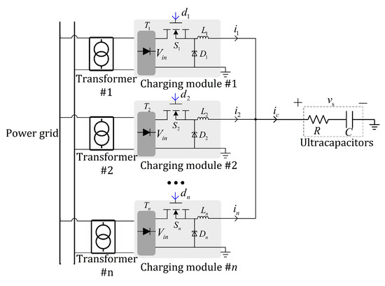
Figure 1.
The scheme of the multi-module charging system.
When the MosFET is on, we have
The matrix expression is
When the MosFET is off, the state equation of buck converter is
The corresponding expression is
Then, the state space average equation can be deduced as follows,
where is the rectified DC input voltage for each charging module, and are the inductor and duty cycle of charging module k, respectively; and and are the average current and voltage of charging module k during the switching cycle, respectively. The symbol is omitted later, but all variables represent the mean of their switching cycles.
As is shown in Figure 1, the topology of entire system consists of multiple charging modules connected in parallel, i.e.,
The system-level state-space model is described as
differential equations are used to describe the charging system. The time-domain model (9) can be converted to a transfer function model. According to the model (9), we have
where is the Laplace transform of charging current , is the Laplace transform of terminal voltage , is the Laplace transforms of output current , and is the Laplace transform of duty cycle of the charging module k.
Then, (10) can be simplified by eliminating the variable as
We define as the output of system, as the reference and as input of system. Therefore, the , , and can be written as follows,
Now, the matrix form of the physical layer model is derived as
where is the Laplace transform of , is the Laplace transform of , and is
The transfer function matrix from to is
The transfer function model of charging system is established from to . The derivation process is as follows.
Then, we have
As the charging modules is connected in parallel, we have
Now, the transfer function matrix from to is derived as
2.2. Cyber Modeling
In this section, the interconnection topology among n charging modules is described by graph theory. The charging modules are regarded as nodes in graph [21]. If node m can send information to node k, we denote , otherwise . We define an adjacency matrix A to describe the communication relationship among n charging modules, i.e., . The degree matrix which is a diagonal matrix can be defined as , where is the number of the nodes which can send information to node k. is defined as the Laplacian matrix L.
The design objective is to guarantee the charging currents/voltages of each charging module follow the target current/voltage. In order to describe the availability of the reference to charging modules, we define a diagonal pinning matrix G as
where if the reference is available to node k, and otherwise.
The matrices and can characterize the interactions of charging modules. The matrix represents the communication topology of neighbor modules and the matrix indicates whether the modules receive the reference information or not.
There are two prerequisites for the effectiveness of the proposed method: (i) at least one charging module is pinned to the reference and (ii) the communication graph of modules is connected.
3. Cooperative Cascade Charging
In this section, a cooperative cascade controller is designed to regulate the charging process of onboard ultracapacitors. The proposed charging scheme consists of an inner current loop and an outer voltage loop. The current loop balances the charging current among charging modules and the voltage loop guarantees the voltage of ultracapacitors follows the reference voltage.
3.1. Cyber-Physical Representation
Figure 2 shows the cyber-physical representation of the proposed charging method, which consists of three layers: physical layer, cyber layer, and control layer. The physical layer mainly includes ultracapacitor stack and multiple parallel charging modules. The sum current of all charging modules serves as the charging current of the ultracapacitor. In the cyber layer, each charging module is regarded as a node in the graph. The connection of the nodes represents that the two modules can communicate with each other. Unlike other nodes, node 0 is a virtual leader representing the reference information. In the control layer, a cooperative control method is designed to eliminate the current imbalance of charging modules.
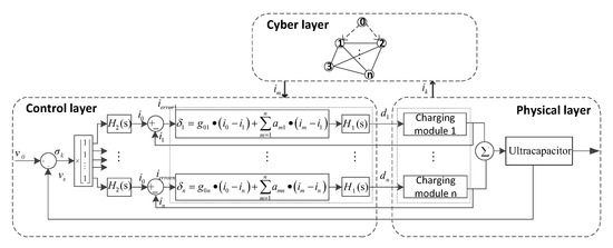
Figure 2.
The cyber-physical representation of the proposed charging control system.
3.2. Cooperative Current Control
The inner current loop is responsible for the constant-current charging. The inner cooperative current controller consists of two terms: a compensator and a cooperative current tracker. The control strategy is shown as follows,
where is the reference current, is the output current of charging module k, is output current of module k’s neighbor, is the pinning gain, and is the adjacent modules.
The reference current is the leader and is the follower. The goal of the cooperative current tracker is that the follower follows the leader while reducing the current difference with it’s neighbors’ current [18].
The second term is the compensator . The input of compensator is the output of the current tracker . The compensator generates duty cycle to ensure the converge to zero. The compensator is shown as follows,
where and are the proportional coefficient and integral coefficient, respectively. The compensator can reduce steady state error and improve the transient response of the charging control system.
Theorem 1.
If the current loop satisfy the following conditions. (i) The reference pins to at least one charging module; (ii) the modules are connected; (iii) the compensator can ensure the formation of a closed-loop system, all followers can be synchronized with the reference finally.
Proof.
From (19), we have
Formula (21) is written in matrix form as
where .
From the definition of the Laplacian matrix, we can know the sum of each row of is zero. Then we have . Adding it to (22) gives the following result:
If the closed-loop system is stable due to the action of compensator , the feedback error will be suppressed to zero. It means that
The matrix is invertible if the reference pin and the module diagram of at least one module are connected.
This completes the proof. ☐
Figure 3 shows the block diagram of the inner cooperative current loop, where the input signal is , and the output is . According to the block diagram, we can obtain the open-loop transfer function matrix as
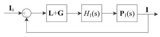
Figure 3.
The control block diagram of the current loop.
The closed-loop transfer function matrix is
where is the identity matrix of order .
3.3. Pinning-Based Voltage Control
Parallel connection is used in charging modules, i.e., the voltage of each module is equal to the voltage of ultracapacitor stack. It means that the ultracapacitor voltage can be controlled by anyone of charging modules.
There are two parts of the outer voltage loop, and the first part is the voltage tracker:
where the is the input of the voltage closed-loop controller, is reference voltage, is the actual output voltage, and is the pinning gain.
The second part is a compensator :
where and are proportional coefficient and integral coefficient, respectively.
3.4. Closed-Loop Modeling
The MIMO model is determined to be the closed-loop model of the whole system. We can use a transfer function matrix to characterize the n-order system.
A control system can be represented by a block diagram which consists of signal lines, lead points, comparison points, and blocks. The signal line is a straight line with an arrow indicating the direction of the signal. The lead point indicates where the signal is taken or measured. Comparison point means the sum or difference of more than two signals. The block indicates the mathematical transformation of the signal, and the transfer function of the component or system is written in the block.
The proposed control system has two main parts: outer voltage loop and inner current loop, where the output of the voltage loop is the reference of inner current loop. The objective of the control system is to ensure the voltage of the ultracapacitor converges to the reference voltage , i.e., the input signal of the system is . The tracking error goes to to generate the reference current . As is a scalar, it is multiplied by a vector to produce . Then, the negative feedback signal generated by is transmitted to the to generate the tracking error . The compensator generates the duty cycle signal according to the current error. Finally, the multi-module charging system obtains the duty cycle signal to provide the output current . The charging block diagram of the system is shown in Figure 4.
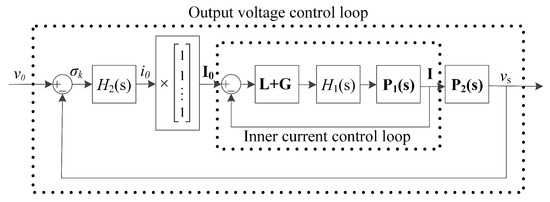
Figure 4.
The closed-loop model of the multi-module charging system.
4. Case Studies
In this section, we evaluate the proposed charging method based on experimental results, and in order to illustrate how to design compensators and , we provide a practical case study. Without loss of generality, we consider the case of three chargers, which can charge ultracapacitors with three chargers connected in parallel.
4.1. Parameter Setting
We first provide the physical and cyber parameters, and then compute the control parameters of and .
4.1.1. Physical Parameters
We design the parameters of the whole charging system: the input voltage V, reference current A, desired voltage V, the capacitance of ultracapacitors F, the ESR of ultracapacitors , and three inductors mH.
4.1.2. Cyber Parameters
Without losing generality, we assume that three chargers are interconnected and the three chargers follow the reference signal. In this case, the matrix and matrix are
4.1.3. Control Parameters
The control parameters of in the current control loop are determined first, and then the control parameters of in the voltage control loop are calculated.
Current Compensator Design: From the work in (27), the closed-loop model of the current loop is determined as
where is the component of the closed-loop transfer function matrix in (27).
Then, represents the closed-loop transfer function from reference to the output current of module k, which can be derived as
The transfer function is calculated by Matlab
The transfer function (32) is a standard second-order transfer function in form. The dynamic performance of the system is determined by the parameters and . The natural frequency and damping ratio of (33) are derived as follows,
The time required for a system to stabilize within of the reference signal is called the setting time. In the second-order system, the settling time is approximated as [22,23]
The stabilization time is usually selected as 0.01 s during CC charging. Substituting into (34) and (35), we obtain
The transient response can be improved when the damping ratio is small during the CC charging. We typically choose [22]. On the premise of generality, we choose . Then, from (34)
The parameters and of compensator in the current control loop have been calculated. Next, the parameters of in the voltage control loop will be determined.
Voltage Compensator Design: The current control loop response is extremely fast compared to the outer voltage loop. Thence in the process of modeling the outer voltage loop, the current loop can be approximated that . Analogy to the above derivation (31)–(33), the transfer function of the voltage circuit is
We can compute
Now the parameters and of compensator are also determined. The effectiveness of the compensators and will be verified with simulation and experiment results.
4.2. Simulation Results
By selecting the corresponding module in Simulink, connecting each module with reference to the mathematical model, and adjusting the parameters, we build the Simulink block diagram, where the reference voltage is set to 2.7 V, and the three charging modules charge the capacitor with a total current of 3 A [24].
The total current and the charging voltage of the ultracapacitor are shown in the Figure 5. The total current quickly rises to 3 A. The current drops after the capacitor voltage reaches the reference value. The voltage of the capacitor increases linearly to a reference value and then stabilizes.
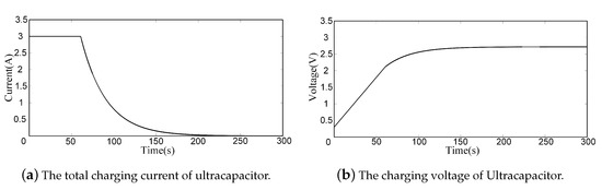
Figure 5.
The total charging current and the charging voltage of ultracapacitor.
As shown in the Figure 6, the three charging modules’ current of the cooperative charging method and the decentralized control method is as follows. If choosing the decentralized control as the method of multi-module charging system, the current among the modules is unbalanced because each charging module operates independently, which reduces the service life of the system. The designed collaborative control method can avoid this situation because the charging current of the three modules are equal.
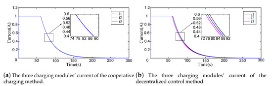
Figure 6.
The three charging modules’ current of two methods.
4.3. Hardware Setup
The experiment platform is shown in Figure 7 which consists of (1) direct current (DC) power source, (2) measurement board, (3) three buck converters, (4) ultracapacitor, (5) PXI platform, and (6) Labview. The charging system consists of one micro-controller, three buck converters, and one ultracapacitor. In this paper, we choose the DSP2808 as the control chip, the controllable DC power supply as the power source [25], and a 100 F ultracapacitor of Maxwell as the load. The PXI platform is used to observe and record the waveform of the ultracapacitor voltage and three chargers’ currents.
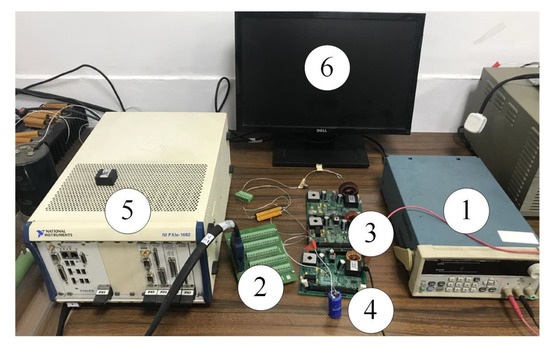
Figure 7.
The hardware setup of the three-charger testbed: (1) power source; (2) measurement board; (3) three buck converters; (4) ultracapacitor; (5) PXI platform; (6) Labview.
The TMS320F2808 is the heart of the control board. It is a fixed-point DSP chip on the C2000 platform introduced by Texas Instruments, and the chip has the advantage of low-cost, low-power, and high-performance processing capabilities. There are 16 PWM outputs, 2 CAN modules, and 16 ADC channels. The measured analog signal is filtered by the operational amplifier TL074ID. In the experiment, we apply one micro-controller to control three charging modules, i.e., the micro-controller consists of three control procedures. The control procedure collects the current of the corresponding charging module and then communicates with each other through the signal flow to make a control decision. The communications among modules are signal flows in the software design.
4.4. Experiment Results
4.4.1. Constant-Current Charging
The constant-current (CC) charging is adopted for fast charging of the ultracapacitors. The current of each charging module and the voltage change of the ultracapacitor are shown in Figure 8. It can be seen from the profiles that the ultracapacitor is charged with a total current of 3 A provided by three charging modules in parallel. When the voltage increases linearly to 2.7 V, the current is disconnected and the charging time is 87 s. Due to the internal resistance of ultracapacitor, the voltage has a sudden drop of 300 mV.
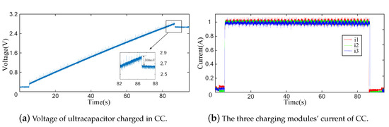
Figure 8.
The CC charging profiles.
4.4.2. Constant Current-Constant Voltage Charging
Cascade charging method can achieve the constant current-constant voltage charging of ultracapacitors when the full charging is required. The charging curves of the charging system are shown in Figure 9, which comprises the voltage profile of the ultracapacitor and current profiles of three charging modules. There are two stages in the charging process: CC charging stage and CV charging stage. In the CC stage, three charging modules supply 1 A output current, respectively. The ultracapacitor is charged with a total current of 3 A, and the voltage increases linearly to the desired voltage 2.5 V. The CC charging protocol is transformed to the CV charging protocol, with the help of algorithm, when the ultracapacitor voltage increases to the desired voltage 2.5 V at 75 s. In the CV stage, the ultracapacitor voltage increases slowly and maintains at 2.7 V. The current of three charging modules decrease to zero exponentially. The ultracapacitor is fully charged and the total charging time is 100 s.
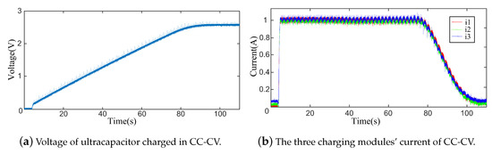
Figure 9.
The CC-CV charging profiles.
4.5. Fault-Tolerant Charging
The superiority of cooperative control is verified with Figure 10, in which we find that the proposed method can reduce the current imbalance effectively. In the decentralized control method, charging modules supply unbalanced charging current. Then, charging modules with larger current will be affected by overload, which will reduce the lifetime of the charging modules and the reliability of the whole charging system will be reduced.
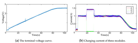
Figure 10.
Fault-tolerant Charging Process.
The control strategy of this paper adopts a distributed structure. The advantage is that it avoids failure of single point and improves the fault tolerance ability of the system. Figure 10b illustrates that during the normal operation of the circuit, the third charging module suddenly fails and the output current becomes zero. When the third charging module fails, the other two charging modules still provide the current required for the ultracapacitor and are not affected by the third charging module. As shown in Figure 10a, the ultracapacitor can be charged to full charge. Due to the failure of other modules, the current of single module may be too high. When the current of a module reaches the limit, we limit its value through the program design to ensure safety.
Due to all of the charging modules are connected with the virtual leader in cyber layer, so the three charging modules work cooperatively to power the ultracapacitor instead of simply paralleling together. From Figure 10b, we can also know that when the third current becomes 0, the current of the ultracapacitor is provided by two charging modules. If the three charging modules are simply connected in parallel, the normal two buck circuit will maintain the original current. In the proposed control scheme of this paper, three parallel current loops are connected in the same voltage loop, so , change from 1 A to 1.5 A when changes from 1 A to 0 A.
At 32 s, where the second charging module is back to normal, Figure 10b shows that returns back to 1 A and , return to 1 A too. Moreover, the slope of the change in ultracapacitor voltage did not change too much during the whole process, and the ultracapacitor voltage rises steadily which is shown in Figure 10a. From Figure 10b we can know the total current of three charging modules is 3 A all the time. It indicates that the faulty of the second charging module has no effect on the normal operation of the system, which confirms the independence among modules of the system.
4.6. Discussions
4.6.1. Effectiveness
In practice, the ultracapacitors can be charged by constant-current (CC) method and constant-current constant-voltage (CC-CV) method. From Figure 8, the charging of CC method is fast but there is a voltage drop of 300 mV at the end of charging. The charging speed of CC-CV method is a little slow but can charge ultracapacitor more fully.
4.6.2. Superiority
As shown in Figure 6, the current imbalance can be restrained by the cooperative charging method which means that the effect is better than that of decentralized control method. The stability and lifetime of the entire charging system are guaranteed. As shown in Figure 10, compared with the classical centralized control method, good scalability, and fault tolerance can be shown in the proposed method.
4.6.3. Scalability
The method proposed in this paper is a cooperative control method. Each charger only communicates with adjacent modules. Therefore, this method has a good scalability. The number of chargers will not affect the stability of the whole system. The proposed method is suitable for multi-module charging applications.
4.6.4. Fault Tolerance
We prove the fault-tolerant ability of the proposed charging system by setting a charging module to fail, and then resume normal operation. As shown in Figure 10. From the figure we can see the failure of second charging module has no effect on the total charging current and ultracapacitor’s voltage, and the entire charging system can still complete the charging task successfully. In addition, Figure 10b also demonstrates the cooperative work ability among charging modules. The output of each charging module is not only related to local information, but also has a relationship with neighbor information.
4.6.5. Communication Delays
The proposed method can be applied in small-scale or large-scale scenarios. In small-scale application, only one micro-controller is needed. The micro-controller can provide the port needed for control without delay problem. In large-scale application where multiple micro-controllers are required, the communication delays between modules will affect the effectiveness of the system.
5. Conclusions
In this paper, we proposed a charging scheme which incorporates cooperative control and cascade control for the ultracapacitor. The cooperative control in the inner current loop of cascade control guarantee that the charging current among charging modules is balanced for the charging system with multiple modules. The outer voltage loop of cascade control can guarantees the ultracapacitor to be charged fully. We also build the block diagram of the proposed control scheme. Moreover, the proposed charging system has a great fault-tolerant ability. The experimental results show the effectiveness of the proposed method. Time delay and synchronization issues of multiple micro-controllers and measurement noises will be considered in our future work.
Author Contributions
Conceptualization, H.L. (Heng Li) and J.P.; methodology, X.Z. and H.L. (Heng Li); validation, J.L.; data curation, J.L. and H.L. (Hongtao Liao); writing–original draft preparation, X.Z. and J.L.; writing–review and editing, H.L. (Heng Li) and J.P. All authors have read and agreed to the published version of the manuscript.
Funding
This research is supported by the National Natural Science Foundation of China (Grant No. 61803394), the National Natural Science Foundation of China (Grant No. 61873353) and the Natural Science Foundation of Hunan Province (Grant No. 2019JJ50822).
Conflicts of Interest
The authors declare no conflict of interest.
References
- Zhang, Y.; Wei, Z.; Li, H.; Cai, L.; Pan, J. Optimal charging scheduling for catenary-free trams in public transportation systems. IEEE Trans. Smart Grid 2017, 10, 227–237. [Google Scholar] [CrossRef]
- Li, H.; Peng, J.; He, J.; Zhou, R.; Huang, Z.; Pan, J. A cooperative charging protocol for onboard supercapacitors of catenary-free trams. IEEE Trans. Control Syst. Technol. 2017, 26, 1219–1232. [Google Scholar] [CrossRef]
- Jabbour, N.; Mademlis, C. Supercapacitor-based energy recovery system with improved power control and energy management for elevator applications. IEEE Trans. Power Electron. 2017, 32, 9389–9399. [Google Scholar] [CrossRef]
- Sun, L.; Feng, K.; Chapman, C.; Zhang, N. An adaptive power-split strategy for battery–supercapacitor powertrain—design, simulation, and experiment. IEEE Trans. Power Electron. 2017, 32, 9364–9375. [Google Scholar] [CrossRef]
- El Mejdoubi, A.; Chaoui, H.; Gualous, H.; Sabor, J. Online parameter identification for supercapacitor state-of-health diagnosis for vehicular applications. IEEE Trans. Power Electron. 2017, 32, 9355–9363. [Google Scholar] [CrossRef]
- Zhang, Q.; Deng, W.; Li, G. Stochastic control of predictive power management for battery/supercapacitor hybrid energy storage systems of electric vehicles. IEEE Trans. Ind. Inform. 2017, 14, 3023–3030. [Google Scholar] [CrossRef]
- Zhang, Q.; Li, G. Experimental study on a semi-active battery-supercapacitor hybrid energy storage system for electric vehicle application. IEEE Trans. Power Electron. 2019, 35, 1014–1021. [Google Scholar] [CrossRef]
- German, R.; Sari, A.; Briat, O.; Vinassa, J.M.; Venet, P. Impact of voltage resets on supercapacitors aging. IEEE Trans. Ind. Electron. 2016, 63, 7703–7711. [Google Scholar] [CrossRef]
- Naseri, F.; Farjah, E.; Ghanbari, T.; Kazemi, Z.; Schaltz, E.; Schanen, J.L. Online parameter estimation for supercapacitor state-of-energy and state-of-health determination in vehicular applications. IEEE Trans. Ind. Electron. 2019, 67, 7963–7972. [Google Scholar] [CrossRef]
- Parvini, Y.; Vahidi, A.; Fayazi, S.A. Heuristic versus optimal charging of supercapacitors, lithium-ion, and lead-acid batteries: An efficiency point of view. IEEE Trans. Control Syst. Technol. 2017, 26, 167–180. [Google Scholar] [CrossRef]
- Yıldırım, D.; Akşit, M.H.; Yolaçan, C.; Pul, T.; Ermiş, C.; Aghdam, B.H.; Çadırcı, I.; Ermiş, M. Full-Scale physical simulator of all SiC traction motor drive with onboard supercapacitor ESS for Light-Rail public transportation. IEEE Trans. Ind. Electron. 2019, 67, 6290–6301. [Google Scholar] [CrossRef]
- Uno, M.; Tanaka, K. Single-switch multioutput charger using voltage multiplier for series-connected lithium-ion battery/supercapacitor equalization. IEEE Trans. Ind. Electron. 2012, 60, 3227–3239. [Google Scholar] [CrossRef]
- Luo, X.; He, J.; Zhu, S. On-board supercapacitors cooperative charging algorithm: Stability analysis and weight optimization. In Proceedings of the IEEE 2020 American Control Conference (ACC), Denver, CO, USA, 1–3 July 2020; pp. 4975–4980. [Google Scholar]
- Ibanez, F.M. Analyzing the need for a balancing system in supercapacitor energy storage systems. IEEE Trans. Power Electron. 2017, 33, 2162–2171. [Google Scholar] [CrossRef]
- Shili, S.; Hijazi, A.; Sari, A.; Lin-Shi, X.; Venet, P. Balancing circuit new control for supercapacitor storage system lifetime maximization. IEEE Trans. Power Electron. 2016, 32, 4939–4948. [Google Scholar] [CrossRef]
- Maneesut, K.; Supatti, U. Reviews of supercapacitor cell voltage equalizer topologies for EVs. In Proceedings of the 2017 IEEE 14th International Conference on Electrical Engineering/Electronics, Computer, Telecommunications and Information Technology (ECTI-CON), Phuket, Thailand, 27–30 June 2017; pp. 608–611. [Google Scholar]
- Ding, L.; Han, Q.L.; Sindi, E. Distributed cooperative optimal control of DC microgrids with communication delays. IEEE Trans. Ind. Inform. 2018, 14, 3924–3935. [Google Scholar] [CrossRef]
- Choi, J.; Oh, S.; Horowitz, R. Distributed learning and cooperative control for multi-agent systems. Automatica 2009, 45, 2802–2814. [Google Scholar] [CrossRef]
- Li, H.; Zhang, X.; Peng, J.; He, J.; Huang, Z.; Wang, J. Cooperative CC-CV charging of supercapacitors using multi-charger systems. IEEE Trans. Ind. Electron. 2020, 67, 10497–10508. [Google Scholar] [CrossRef]
- Li, Q.; Su, B.; Pu, Y.; Han, Y.; Wang, T.; Yin, L.; Chen, W. A state machine control based on equivalent consumption minimization for fuel cell/supercapacitor hybrid tramway. IEEE Trans. Transp. Electrif. 2019, 5, 552–564. [Google Scholar] [CrossRef]
- Olfati-Saber, R.; Fax, J.A.; Murray, R.M. Consensus and cooperation in networked multi-agent systems. Proc. IEEE 2007, 95, 215–233. [Google Scholar] [CrossRef]
- Ogata, K.; Yang, Y. Modern Control Engineering; Prentice Hall India: New Delhi, India, 2002; Volume 4. [Google Scholar]
- Pavković, D.; Polak, S.; Zorc, D. PID controller auto-tuning based on process step response and damping optimum criterion. ISA Trans. 2014, 53, 85–96. [Google Scholar] [CrossRef]
- Newman, P.; Hargroves, K.; Davies-Slate, S.; Conley, D.; Verschuer, M.; Mouritz, M.; Yangka, D. The trackless tram: Is it the transit and city shaping catalyst we have been waiting for? J. Transp.Technol. 2018, 9, 31–55. [Google Scholar] [CrossRef]
- Ren, W.; Beard, R.W.; Atkins, E.M. Information consensus in multivehicle cooperative control. IEEE Control Syst. Mag. 2007, 27, 71–82. [Google Scholar]
© 2020 by the authors. Licensee MDPI, Basel, Switzerland. This article is an open access article distributed under the terms and conditions of the Creative Commons Attribution (CC BY) license (http://creativecommons.org/licenses/by/4.0/).