Big Data Analytics for Short and Medium-Term Electricity Load Forecasting Using an AI Techniques Ensembler

Abstract

Electrical load forecasting provides knowledge about future consumption and generation of electricity. There is a high level of fluctuation behavior between energy generation and consumption. Sometimes, the energy demand of the consumer becomes higher than the energy already generated, and vice versa. Electricity load forecasting provides a monitoring framework for future energy generation, consumption, and making a balance between them. In this paper, we propose a framework, in which deep learning and supervised machine learning techniques are implemented for electricity-load forecasting. A three-step model is proposed, which includes: feature selection, extraction, and classification. The hybrid of Random Forest (RF) and Extreme Gradient Boosting (XGB) is used to calculate features’ importance. The average feature importance of hybrid techniques selects the most relevant and high importance features in the feature selection method. The Recursive Feature Elimination (RFE) method is used to eliminate the irrelevant features in the feature extraction method. The load forecasting is performed with Support Vector Machines (SVM) and a hybrid of Gated Recurrent Units (GRU) and Convolutional Neural Networks (CNN). The meta-heuristic algorithms, i.e., Grey Wolf Optimization (GWO) and Earth Worm Optimization (EWO) are applied to tune the hyper-parameters of SVM and CNN-GRU, respectively. The accuracy of our enhanced techniques CNN-GRU-EWO and SVM-GWO is 96.33% and 90.67%, respectively. Our proposed techniques CNN-GRU-EWO and SVM-GWO perform 7% and 3% better than the State-Of-The-Art (SOTA). In the end, a comparison with SOTA techniques is performed to show the improvement of the proposed techniques. This comparison showed that the proposed technique performs well and results in the lowest performance error rates and highest accuracy rates as compared to other techniques.

1. Introduction

The electrical industry plays a very vital role in human life from various angles. The electricity demand is increasing day-by-day with the rapid increase in population [1]. The traditional power grid became an old version; which is not efficient enough now, so, the intelligent and smart version of the power grid known as the Smart Grid (SG) is introduced. Through the SG system, it became very easy to manage the distribution of electric load for utility companies and remain in touch with the consumers. The SG also helps to reduce the variations between power demand and supply. The most important task of the SG is to effectively control the consumption, generation, and distribution of electricity. The utility supplies electricity to consumers, according to their demand. Sometimes, the rate of electricity consumption of the user increases and the utility does not have enough energy be supplied. To overcome the issue of balancing between consumption and utility supply, the utility uses the electricity load forecasting model, which is one aspect of SG. The conceptual diagram of the SG is shown in Figure 1.

Figure 1. Smart grid infrastructure.

The approximate energy consumption pattern of the user is predicted through load forecasting by their historical data. Generally, forecasting is of four types; Short-Term Forecasting (STF), Very Small Term Forecasting (VSTF), Medium-Term Forecasting (MTF), and Long-Term Forecasting (LTF). In STF, electric load of one day-ahead to some weeks-ahead is predicted, VSTF consists of predictions for some hours to one day, MTF predicts data of one week to one year, and through LTF, one year to several years ahead load can be forecasted [2,3,4]. In this paper, STF and MTF are performed with an excessive record of electricity dataset. Data analysis is a process of getting useful information from hidden patterns of data. Data analysts measures the price and load consumption by taking historical data in the form of datasets to perform some tasks which allow us to obtain useful information [5]. In [6], the detailed review of data is available. The volume of real-world data is intensively increasing day-by-day and the large volume of data is referred to as big data. Through data analytics, effective information is collected from massive quantities of historical power data to implement analysis over it, which helps to make more enhancements in the market operations management and planning. Big data is multifaceted and very excessive in volume. The main issue in the big data sets is redundant features; so traditional methods are not very supportive for handling such a large amount of data.

Many techniques are tested and applied to handle big data and extract useful information. Although, big data is still an issue of the current era. Many authors around the globe are working on handling big data using artificial intelligence techniques. The authors in [7,8] improved the price forecasting and load forecasting accuracy; however, the computational time is not considered. Similarly, the issue of load forecasting is addressed in [9]; however, the issue of overfitting is not addressed. Moreover in [10], the author proposed the BPNN model to forecast the day-ahead electricity load; however, the complexity of the proposed model is increased. Additionally, the LSTM-RNN model in [11] is used to forecast an hourly and monthly electricity load. Furthermore in [12], the hybrid of SVM and non-linear regression is used to forecast load; unfortunately, the problem of over-fitting is increased. Hence, conventional simple techniques and methods are not very suitable for a varying electricity load. A better framework and enhanced techniques are required to solve the load forecasting problem. Therefore, the main objective of this paper is to enhance the accuracy rate of electricity load forecasting by optimizing the parameters of machine learning and deep learning techniques on a large amount of electricity load data. As a large amount of data contain redundant and irrelevant features, which increase the time complexity of training. RF and XGB are used as feature selection methods. The RFE technique is used as a feature extraction method to eliminate the redundancy, while SVM with the GWO algorithm and CNN-GRU with the EWO algorithm is used for the classification of electricity load forecasting.

The main contributions of this paper are given below:

• Hybrid of feature selection techniques; Extreme Gradient Boosting (XGB), Random Forest RF and Recursive Feature Elimination (RFE) techniques are applied to clean the huge amount of data.
• Two enhanced classifier techniques, Support Vector Machine with Grey Wolf Optimization (SVM-GWO) and Convolutional Neural Network Gated Recurrent Unit with Earth Worm Optimization (CNN-GRU-EWO) are proposed to forecast the electricity load.
• Grey Wolf Optimization (GWO) and Earth Worm Optimization (EWO) algorithms are used to tune the parameters of SVM and CNN-GRU, respectively.
• The parameters of classifiers are tuned to reduce the computational time efficiently.
• To overcome the overfitting problem, enhanced classifiers are used.
• Our proposed techniques are compared with some State Of The Art (SOTA) to prove the better performance of our enhanced techniques.

The rest of the paper is organized as follows. Section 2 contains the literature review. Section 3 contains the proposed methodology (method). Section 4 contains the results. Section 5 contains the conclusion and policy implications.

2. Related Work

Many techniques and ideas are used and tested to predict the power load and other areas with successive results. In [13], the authors performed load forecasting with various smart home data by applying an analytical approach to the data, however, they were unable to manage a large amount of data properly. Deep Long Short Term Memory (DLSTM) and machine learning-based model are proposed to forecast the price and electricity [14]. The proposed DLSTM outperforms in achieving the accuracy of load forecasting. However, LSTM is not good in terms of training because it needsa memory bandwidth bound calculation and it limits the applicability of neural network solutions.

In [15], the authors performed load forecasting with feature selection and classification models, taking the dataset as input. They used MI to select the best features and discard insignificant features. The authors proposed three-step strategies for load forecasting in [16], in the first step they used Conditional Mutual Information (CMI) for best feature selection. The second step consists of NLSSVM and ARIMA machine learning techniques, which create nonlinear and linear correlations for load forecasting. In the third step, the parameters of NLSSVM are tuned with the ABC algorithm. However, reducing the features with the help of a feature selection method also reduces the forecasting accuracy rate.

For feature selection, IG and MI techniques have been used, which helped measure the redundancy and most relevant features [17]. They also proposed a hybrid wrapper filter-based approach, where the filter part of the method is selected as a little part of the dataset for features by redundancy and iteration of inputs. They introduced a new feature selection method, but failed to maintain high accuracy rates.

The authors in [18] performed hourly forecasting and also defined the uncertainty of the predictive method. They proposed Generalized ELM and Improve WNN techniques to implement on OAE electrical dataset. However, these techniques are outperformed for this development. The parameters of these techniques are manually tuned, however, with dynamically-tuned hyper-parameters, forecasting accuracy rates can be further increased.

In [19], forecasting has been done using a combination of two deep learning techniques; CNN and LSTM. The proposed model is evaluated using the Mean Square Error (MSE). Further, the accuracy rate of the proposed technique also compared with some benchmark techniques, and results show that the proposed technique outclasses all other techniques in terms of the accuracy rate. The proposed technique performed better, but the authors did not consider the feature redundancy. Redundant features can make a negative effect on model accuracy rates.

The authors in [20], performed day-ahead forecasting by increasing the layers of Artificial Neural Networks (ANN) and tuned the hyper-parameters with an optimizing algorithm. To improve the accuracy rate authors in [21] increased the layers of Neural-Network (NN). The enhanced NN is also compared with conventional techniques to demonstrate improved high accuracy rates. The enhanced NN is compared with ARIMA and SVR, showing that it performed better, but failed to avoid overfitting problems.

In [22], each day of the week forecasting is performed by applying the deep CNN for classification. The applied dataset is taken from the Victorian electrical company, Australia. The authors forecast the one day load and analyzed it by comparing the one day load with the same day’s load of the previous three months. However, the author used fewer record datasets and was unable to train the CNN model properly.

The hybrid of CNN and LSTM achieved accuracy in terms of electricity load forecasting in [23]. The objective of their work is short-term forecasting and they used MAPE and MAE error metrics for evaluation of results. The hyperparameters of SVM are tuned with a random search algorithm to achieve improved accuracy and a lower error rate [18]. They performed load forecasting and compared the results with manually tuned SVM and CNN. Results show the improvement of the enhanced technique. The authors used eight years of data for load forecasting purposes, however, SVM is not good for classifying large datasets.

In [24], the authors proposed two techniques named enhanced SVM and enhanced ELM to perform short term load forecasting. A grid search optimization algorithm is used to optimize the hyper-parameters of SVM and the hyper-parameters of the Extreme Learning Machine (ELM) tuned with the Genetic Algorithm (GA). The proposed techniques performed better, but the authors failed to avoid overfitting problems for SVM.

The short-term load forecasting is performed using NN and Levenberg Marquardt learning in [25]. The authors used the Tanzanian dataset duration 2000 to 2008. The author used MAE, MAPE, MSE, and MAPE error matrices to calculate the result. However, the calculated results through MPE and MAPE gave good results, but the error rates calculated through MAE and MSE are very high.

The authors performed forecasting based on a feature selection technique and least square SVM technique in [26]. They used ASF to select the most informative input values and least square SVM used to predict the model. Results were evaluated with MAPE and MAE error metrics. The proposed model gave low error rates concerning MAPE values, but through MAE it showed the worst results. The authors in [27] performed forecasting with feature selection and classification model. Feature selection was based on MI and CA. The classification part was based on the iterative approach of two neural networks. They used the output of the first neural network as an input of the second neural network.

The consumption data of homes are obtained through smart meters and used to perform forecasting with the help of the GRU deep learning technique in [28]. The authors did not consider preprocessing the dataset and did not remove irrelevant features through their applied model. In [29] authors used hourly and historical temperature data for forecasting. The SVM and ANN machine learning techniques are proposed for this purpose. However, the parameters of thr proposed techniques have been tuned manually.

Improved kernel ELM and Cholesky decomposition techniques are used to forecast the electrical load in [30]. The proposed technique is further compared with conventional ELM and GNN. RMSE error evaluator has used to evaluating the results. In their research work, only one evaluator is used to prove the superiority of the proposed model, other error metrics such as MAPE, RMSE, MSE, accuracy, f1-score, and precision, etc. are not included.

In [31,32], authors used the enhanced CNN method to forecast the electricity load. Furthermore, the superiority of the proposed method is shown with different statistical tests. A composite method based on the optimal learning MLP technique is applied to forecast the mid-term electricity load [33,34]. An acceptable accuracy of 85% is achieved to forecast the mid-term electricity load. However, the author has not considered the overfitting problem of MLP and was unable to highlight the issue of disregarding spatial information.

The deep learning techniques CNN and ANN are used for forecasting in [35,36]. The authors tuned the parameters manually and did not eliminate the irrelevant features. The hybrid of CNN and GRU is applied to predict the electricity load in [37,38,39]. Results are evaluated with MAPE and RMSE values. A comparison of the hybrid technique and conventional techniques also performed. Comparison results show that the hybrid technique outclasses all other techniques. The hybrid model performed well, but parameters have been manually tuned. In our work, we have used the latest heuristic algorithm to automatically allocate the optimum values to the parameters of our proposed techniques. In [40,41], the authors used a framework named feature selection, extraction and classification for load forecasting. They used a hybrid of XGB and DTC techniques to select the most relevant features and eliminated the irrelevant features in the feature extraction step using RFE technique. In the end, classification is performed using SVM. The proposed framework performed well, but the computational complexity of SVM is high and SVM is also not good for processing uncertain data [42,43,44]. The literature review shows that most authors performed forecasting with machine learning and deep learning Table 1. By finding the optimal value for the hyperparameters of techniques is tough work. Furthermore, the irrelevant features in electricity datasets also have a negative impact on model training. To solve some of the above-mentioned issues, we used heuristic algorithms to find optimal values of hyperparameters automatically and for feature selection, the extraction model was proposed to remove irrelevant features from a dataset.

Table 1. Tabular form of related work.

Proposed Techniques	Objective	Dataset	Limitations
DA [13]	Reduce peak load	PJM	Issue in managing big data
DLSTM [14]	Price and Load forecasting	ISO-NE	Cannot fulfill the requirement of real time data.
CMI, NLSSVM [15,16]	Forecasting with important feature selection method	PJM	Less amount of data is taken into consideration
GELM, IWNN [17]	Hourly price forecasting	PJM	Model complexity is considered
CNN, LSTM [18,19]	Price forecasting	PJM	Redundancy in features are not considered
DNN [20]	Load forecasting	Irish	Overfitting problem needed to improve
DCNN [21]	Load forecasting of one day	Victoria	Limited use of dataset
ESVM [22,23]	Short term load forecasting	ISO-NE	SVM is not good to deal big dataset because overfitting problem
ANN [24]	Half hourly load forecasting	Tanzanian	Accuracy rates of their work are not satisfactory.
MI, NN [25]	Short term forecasting	PJM	Maximize the penetration of renewable energy
NARX, ARMAX [26]	Residential based short term load forecasting	IESCO	Model complexity increased
GRU [27]	Load forecasting	PJM	Redundancy of features did not considered
SVM, ANN [28]	Short term forecasting	IITK	Very small dataset is used for experiment
ELM-K [29]	Short term forecasting	Southern China	Only one error metrics used for evaluation.
CNN [20]	Short term forecasting	ISO-NE	Manually tuned the hyper parameters of proposed technique
GRU-CNN [31]	Short term forecasting	Wuwei, Gansu province	Manually tuned the hyper parameters of proposed technique
MI, ANN [32]	Day ahead load forecasting	DAYTOWN, AKPC	Feature selection need more improvement

3. Proposed System Model

After evaluating the literature review and the aforementioned techniques for load forecasting, we propose a framework that is based on average feature selection, extraction, and forecasting. The machine learning techniques, RF, and XGB are used as feature selection techniques, while RFE is used for feature extraction activity. For average feature selection, the average score of RF and XGB is considered for the selection of features as described in Equation (1). Moreover, for classification purposes, machine learning-based technique SVM and deep learning-based technique CNN-GRU are used, respectively. Furthermore, the basic parameters of the CNN-GRU and SVM are tuned with a meta-heuristic algorithm, i.e., EWO and GWO, respectively. The forecasting in Figure 2 displayed the working flowchart of the used model.

Figure 2. Detailed flowchart of the proposed model.

3.1. Dataset Description

The latest electricity daily load dataset is used in this paper, which is downloaded from the ISONE website [34]. The columns in the dataset are referred to as “features” in our work. The dataset is organized according to a month-wise pattern, i.e., January 2012, January 2013 up to January 2019 and February 2012, February 2013 up to February 2019, and so on. The benefit of the month-wise organization is to improve the performance and learning rate of training activity on the dataset.

The dataset set contains 14 features. A feature named “System Load” is taken as a label, i.e., target feature. We used 70% of data in the dataset for training and 30% of data for testing our proposed model. Afterwards, the dataset was again divided; 90% for training and 10% for testing. The testing includes the one-week, one-month and four-month prediction, which are shown in the simulation section. The autocorrelation of data is shown in Figure 3. The overview of the dataset is shown in Figure 4.

Figure 3. Autocorrelation of input data.

Figure 4. Dataset Overview (Features and Labels).

3.2. Feature Engineering

Machine learning techniques XGB lnd RF are used for the selection of relevant features. RF and XGB calculate the features’ importance, i.e., the impact of all features on the target feature. The values are calculated in decimals between 0 and 1. To make the feature selection better, the average of feature importance is taken as given in Equation (1). The feature engineering step removes the unnecessary features and reduces the complexity of the proposed model by providing exact and relevant features for training.

$$Fs=\frac{Fi\left(XGB\right)+Fi\left(RF\right)}{2}$$

(1)

Whereas, Fs defines feature selection and Fi describes the feature importance.

After the selection of relevant features, the most redundant features are extracted using the RFE technique. The RFE technique calculates the dimension and priority of features in terms of true/false and positive integer numbers. After calculating the feature importance through feature selection and dimensional conversion with feature extraction, the drop-out rate is set to eliminate unimportant features. According to Equation (2), those features are selected/reserved, whose average feature importance/weight is greater than the defined threshold and the priority of feature is higher than the defined priority threshold. Moreover, those features are rejected/dropped whose feature weight is fewer than defined feature importance selection threshold and priority are greater than the defined feature priority threshold. The selection threshold of features using average feature selection is 0.6. Furthermore, the features with a priority greater than 5 are considered for selection. The overall selection of features is carried out according to the Equation (2).

$$Fos=\sum _{fr=0}^n\left\{\begin{array}{cc}reserveFeature,& {avg}_{imp}\left(f\right)\ge \alpha \&RFE{\left(f\right)}_{pr}\le \beta pr\hfill \\ dropFeature,& {avg}_{imp}\left(f\right)\ge \alpha \&RFE{\left(fr\right)}_{pr}>\beta pr\hfill \end{array}\right.$$

(2)

Whereas, Fos denotes the overall feature selection and f indicates the feature. avgimp denotes the average feature importance while pr represents the priority of the feature. The $\alpha$ and $\beta pr$ describe the feature importance threshold and feature priority threshold. After feature selection and extraction, the most relevant features are passed to the classifier for classification and forecasting.

3.3. Classification and Forecasting

The classification is carried out using machine learning, i.e., SVM and deep learning CNN-GRU techniques set tuned with optimization techniques, i.e., GWO and EWO, respectively. The tuning parameters of SVM are loss function (gamma), cost incentive (C), and kernel function. The tuning parameters of CNN-GRU are numbers of hidden layers, numbers of neurons on each layer, dropout value. The tuning step will provide optimum values to the classifier, which results in the best training of the model and reduces the chance of overfitting the model on a large amount of data.

3.3.1. CNN-GRU-EWO

The hybrid of CNN and GRU has been used, further, the parameters of this hybrid model are tuned with the EWO technique. The output shape of tuned CNN-GRU layers is shown in Figure 5. The detailed description of CNN and GWO is given below.

Figure 5. Output shape of tuned Convolutional Neural Network (CNN) layers.

Convolutional Neural Network: CNN is a type of deep learning algorithm. This technique is widely used in text and image recognition [29]. CNN might have multiple hidden layers between a single input and the output layer. The hidden layers are convolutional, dense, max-pooling, dropout, and flatten.

Input Layer: This layer is used as the beginning of the workflow of proposed CNN. It is used as a 1st layer of the network. It has no previous layer, nor any weight input. The number of neurons and dataset features is equal at this stage.

Hidden Layer: There can be multiple hidden layers on CNN. The output of the first layer is given to these hidden layers. Each hidden layer can have a different number of neurons. The output of these layers is evaluated with the multiplication of matrices and with previous layers output.

Output Layer: The hidden layer’s output becomes the input of this layer. Softmax or sigmoid and logistic functions are used to transfer this input into the probability score.

Convolutional Layer: This layer has multiple filters and performs the most computational work. The convolutional operation is performed through this layer and results are given to the next layer.

Dense Layer: It acts as a conventional MLP. It is directed to connect the neuron of one layer with any other layers’ neurons.

Pooling Layer: This layer is used for combining the output of neurons. Further, it is divided into three types; average-pooling, max-pooling, sum-pooling. In our model, max-pooling is used to minimize the parameters and reduce calculation. Generally, this layer is used between convolutional and drop layers.

Activation Function: The activation function Rectified-Linear-Unit (ReLU) is used in the convolutional layer.

3.3.2. Gated Recurrent Unit (GRU)

GRU is an updated version of the Recurrent Neural Network (RNN). RNN has a problem with short term memory, in this context, LSTM and GRU have been proposed. Both GRU and LSTM are useful for maintaining long term information with the help of a gating mechanism. LSTM consists of three gates and GRU just has two gates, named update gate and reset gate [30].

Update Gate: This gate helps the model to calculate how much previous information is needed to be passed in the future. The update gate is very useful for eliminating the risk factor of the vanishing gradient problem because it remembers past information and decides which information is useful and which is not.

Reset Gate: This gate is used to decide how much of the previous information to forget.

CNN-GRU: CNN is useful to handle high-dimensional datasets and GRU is useful to process sequence data in minimum time. With the hybridization of these techniques, we can achieve both qualities. In this paper, a hybrid of CNN and GRU is proposed. In this proposed model, the output of the feature selection and extraction is given to CNN. After the input layer of CNN, a GRU is placed. After that, fully connected hidden layers are placed. In the end, the model is compiled and trained to get predicted results.

EWO: To tune the hyperparameters of CNN-GRU, the EWO optimization technique is used as shown in Figure 6. EWO is a nature-inspired heuristic algorithm that is used to solve the optimization problem. In this technique, every earthworm can produce offspring of only two kinds. The child earthworm contains the same length gene as his parent earthworm has. Some earthworms have the best fitness and forward this best fitness to the next generation without any change.

Figure 6. CNN-GRU-GWO.

3.3.3. SVM-GWO

To improve the performance of the machine learning technique SVM, the hyperparameters of SVM are tuned with the GWO optimization algorithm.

SVM: It is a type of supervised machine learning algorithm. It is widely used to solve the classification and regression problems. In SVM, a hyperplane line is drawn as in Figure 7, to divide the features into two classes; Linear and Non-Linear. In our proposed SVM, the parameter “gamma”, i.e., loss function used with kernel RBF. After tuning the SVM, the optimization technique GWO calculated an optimum value for the SVM parameters; the value of gamma is 0.1, and the value of C is 1.0.

Figure 7. Support Vector Machine (SVM).

GWO: It is the part of the metaheuristic and swam optimization family. To tune the parameters of the SVM technique, GWO is used. This technique is developed by [31] in 2014, the authors were inspired by the grey wolf’s social behavior and named this technique based on the “Grey Wolf Optimization”. The hybrid of SVM and GWO is shown in Figure 8.

Figure 8. SVM-Grey Wolf Optimization (GWO).

4. Simulation Results

The complete implementation of our proposed framework was carried out on the system with specification; Intel Core i7, 8 GB RAM, dual 2.4 GHz Processor, built-in GPU Intel 5200, and 1TB SSD. The simulation was carried out on software named Anaconda Spyder and the python language environment with packages including Keras v2.3.1, Tensorflow v2.0, pyswarm v1.1.0, mealpy v0.3.0, pandas v1.0.3, and numpy v1.18.4. The simulation results are shown in figures and tables.

4.1. Average Feature Selection Based on RF and XGB

Feature importance calculated by XGB and RF is shown in Figure 9. Features with more importance have high values and less important features have low values. To make selection feasible and effective, the average feature importance was calculated from RF and XGB feature importance as shown in Figure 10. The features which had higher importance than the threshold were selected and low importance features were rejected. The feature importance calculated by RF is shown in Figure 9a, which shows it’s Demand and the Dewpoint feature was most important in the dataset and high impact on the target data. Figure 9b shows the feature score calculated using XGB, which gives RT_CC and Demand as the most relevant feature. The average of Figure 9a,b is taken to calculate the average importance, which is shown in Figure 10. According to the average calculation of features, Demand, RT_MLC, DA_MLC and Dewpoint are the most relevant feature with high influence on the target feature.

Figure 9. Feature importance calculated by (a) Random forest (b) Extra Gradient Boosting.

Figure 10. Average feature importance.

RFE calculates the dimensions of the features, i.e., true/false, and thus it removes the redundant features from the dataset. The threshold set for feature selection and extraction is the features with average importance greater than 0.6 and dimension true, which were selected as the best features, while importance less than 0.6 and false dimension were rejected features. Table 2 shows the feature dimensions calculated by RFE. Furthermore, the abbreviation of features is also described.

Table 2. Features overview and dimensions calculated by Recursive Feature Elimination (RFE).

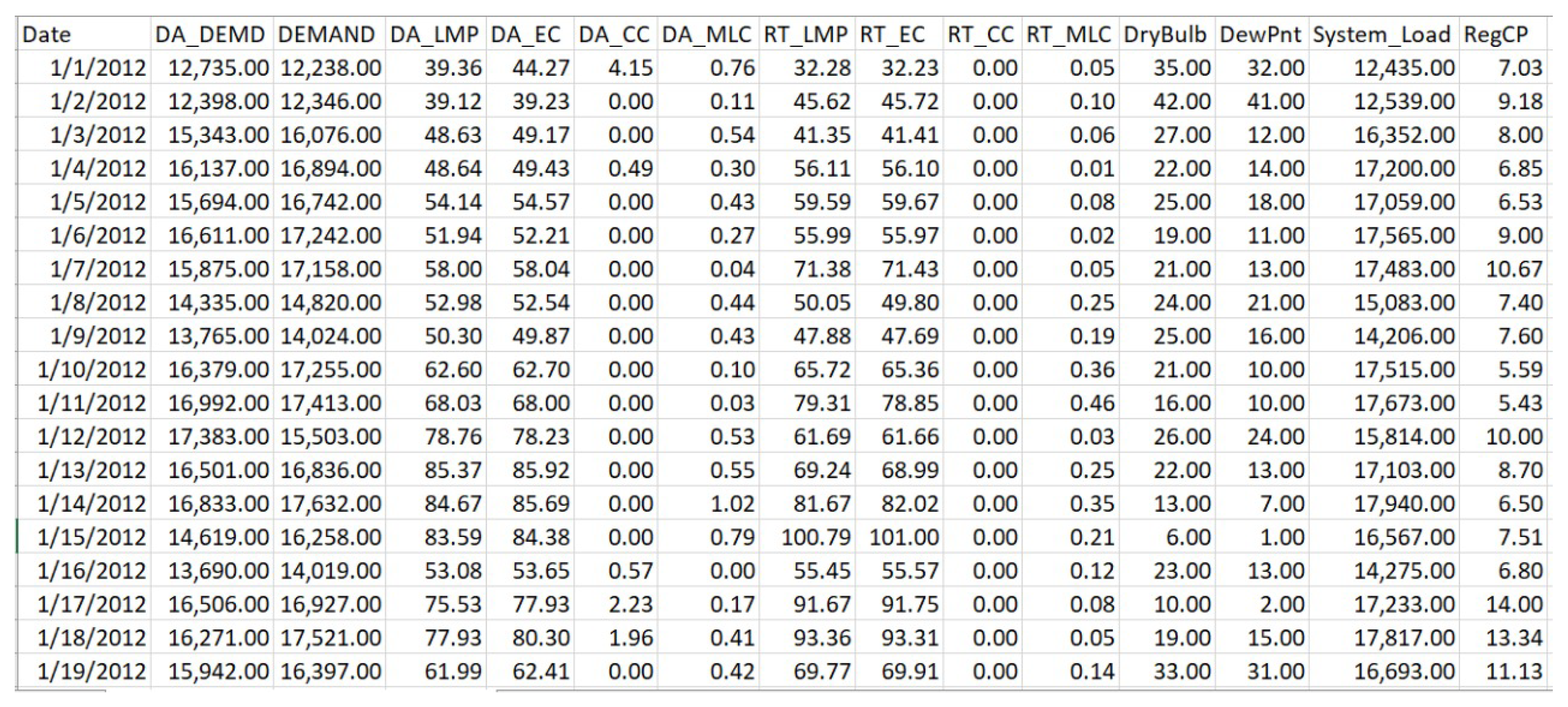
Target Feature	Features	Short Name	Dimension
System Load	Day-Ahead Cleared Demand	DA_Demand	TRUE
	Regulation Market Service clearing price	Reg_Capacity_Price	TRUE
	Real-Time Demand	RT_Demand	TRUE
	The dewpoint temperature	Dew_Point	FALSE
	Day-Ahead Locational Marginal Price	DA_LMP	FALSE
	The dry-bulb temperature	Dry_Bulb	FALSE
	Energy Component of Day-Ahead	DA_EC	FALSE
	Marginal Loss Component of Real-Time	RT_MLC	FALSE
	Congestion Component of Day-Ahead	DA_CC	FALSE
	Congestion Component of Real-Time	RT_CC	FALSE
	Marginal Loss Component of Day-Ahead	DA_MLC	FALSE
	Energy Component of Real-Time	RT_EC	TRUE
	Real-Time Locational Marginal Price	RT_LMP	TRUE
	Regulation Market Capacity clearing	Reg_Service_Price	FALSE

4.2. Classification and Forecasting Using SVM-GWO and CNN-GRU-EWO

Figure 11 shows the normal electricity load data from 1 January 2019 to 31 December 2019, which is provided by ISONE.

Figure 11. Normal electricity load.

The data is arranged month-wise, as the load pattern of similar months are approximately the same, which is shown in Figure 12. The monthly load of the Jan 2018 and Jan 2019 is approximately the same. Similarly, the load pattern of Dec 2018 and Dec 2019 are almost the same. The same pattern of load helps in the training of our model better.

Figure 12. Similar months load pattern.

Figure 13 and Figure 14 describe the prediction of one week, i.e., 1 Feburary 2019 to 7 Feburary 2019 and one month prediction, i.e., March 2019, respectively. The STF and MTF are covered in this paper. While forecasting the first week. All data, except the first week of Feburary 2019, were considered for training. The same case was applied for March 2019. During forecasting the electricity load of March 2019, all data, except March 2019, were considered for training. Figure 13 shows weekly forecast and Figure 14 shows monthly electricity load forecast. Our proposed algorithm performed better in achieving forecasting accuracy.

Figure 13. One-week prediction.

Figure 14. One-month prediction.

In Figure 13 and Figure 14, the prediction values of our proposed techniques were nearly the same as the actual values of electricity load.

Due to efficient training of our proposed techniques on a large amount of data, our proposed model can forecast the load of the upcoming four months, i.e., September 2019, October 2019, November 2019, and December 2019 as shown in Figure 15. While forecasting the electricity load of the last four months of the year 2019, all data except the last four months of the year 2019 are considered for training. The trained model is then tested in the last four months of the year 2019. Our proposed techniques outperform SOTA as shown in Figure 15.

Figure 15. Four-month prediction.

The accuracy of our proposed techniques is higher than the SOTA as described in Figure 16. The enhanced version of the technique outperformed the actual technique. The optimization techniques, i.e., GWO and EWO found the best optimum solutions for the hyperparameters of the techniques, which enhance the accuracy and reduce the time complexity of training the model. The accuracy of our proposed techniques CNN-GRU-EWO and SVM-GWO is 93% and 90%, respectively. The accuracy of SOTA techniques SVM, CNN, LR and ELM is 87.98%, 89%, 78.34%, and 78.98%, respectively, as shown in Figure 16.

Figure 16. Accuracy of proposed techniques vs the State-Of-The-Art (SOTA).

5. Performance Metrics

The performance of our proposed model and SOTA techniques were evaluated using MAPE, MAE, RMSE, MSE, precision, re-call, f-measure, and accuracy. The performance errors of our proposed techniques were much lower than the SOTA as shown in Figure 17. The performance evaluation metrics accuracy was higher than benchmark techniques as shown in Figure 18.

Figure 17. Performance error.

Figure 18. Performance evaluation.

The performance evaluation metrics like precision and recall are calculated using Equations (3) and (4).

$$\mathrm{Precision}=\frac{\mathrm{True}\mathrm{Positive}}{\mathrm{True}\mathrm{Positive}+\mathrm{False}\mathrm{Positive}}$$

(3)

$$\mathrm{Recall}=\frac{\mathrm{True}\mathrm{Positive}}{\mathrm{True}\mathrm{Positive}+\mathrm{False}\mathrm{Negative}}$$

(4)

The performance values i.e., F1-score, accuracy, precision, and recall of CNN-GRU-EWA and CNN-GWO is greater than LG, CNN, SVM, and ELM.

The MAPE error of SVM-GWO and CNN-GRU-EWA is 1.33% and 6%. The LG technique has the highest performance error of 20%. The high-performance error reduces the forecasting accuracy

The training and testing accuracy of our proposed model is shown in Figure 19 and Figure 20. The graph of accuracy is gradually increases with the increase in training on an excessive amount of data. The loss graph is gradually decreased, which shows that our model is well trained and test.

Figure 19. Train–test accuracy.

Figure 20. Train–test loss.

The performance evaluation with the performance metric values of our model is described in Table 3.

Table 3. Performance evaluation results of proposed and benchmark methods.

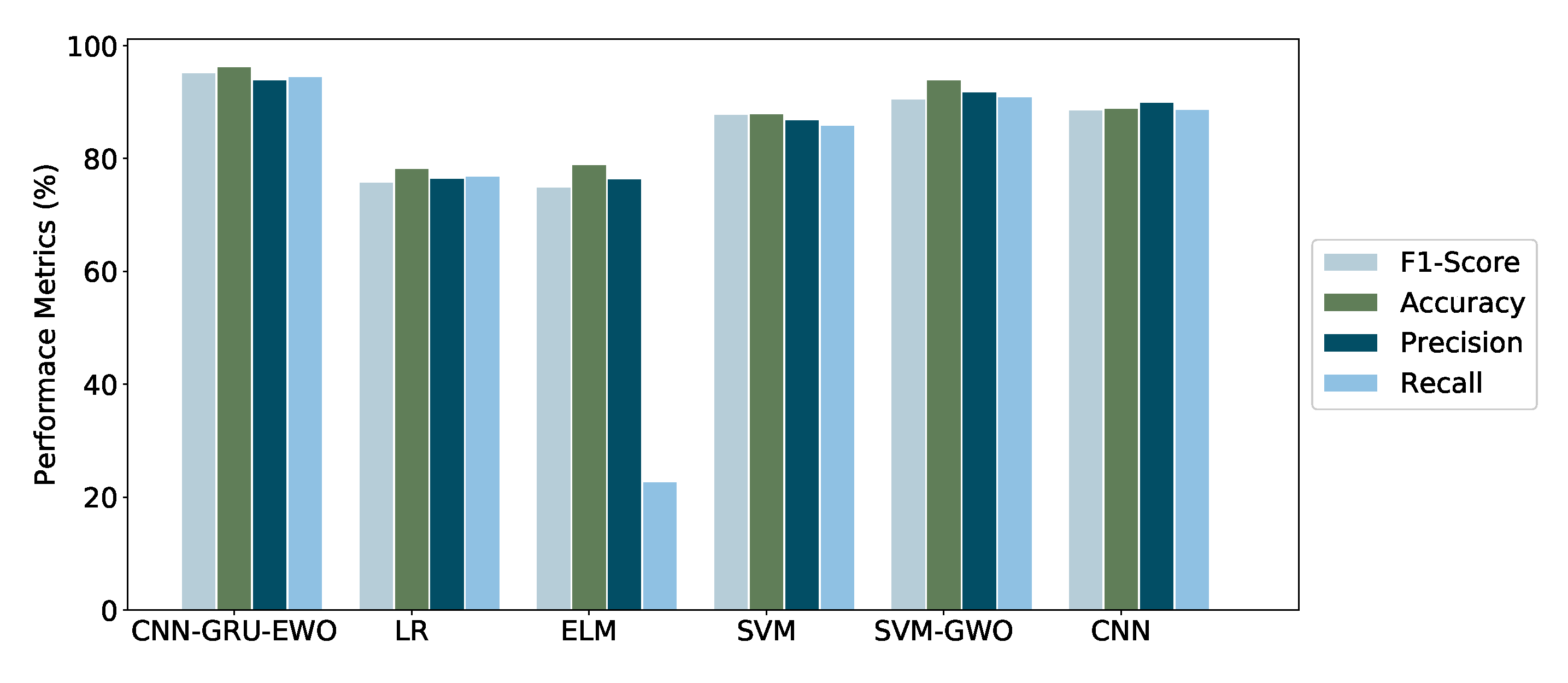
Techniques	Performance Metrics
	F1-Score	Accuracy	Precision	Recall	MAPE	RMSE	MAE	MSE
CNN_GRU_EWA	95.23	96.33	94.00	94.62	6.00	7.00	10.00	13.00
LR	75.88	78.35	76.56	76.98	20.00	23.00	27.00	26.00
ELM	75.00	78.98	76.45	22.78	13.00	12.00	15.00	18.00
SVM	87.88	87.99	86.91	85.99	1.79	12.30	10.50	12.00
SVM_GWO	90.67	93.99	91.87	90.99	1.33	9.12	10.31	9.75
CNN	88.66	89.00	90.00	88.76	10.00	12.00	15.00	18.00

Table 4 shows different correlation-based tests, a parametric statistical hypothesis-based tests and non-parametric statistical hypothesis based statistical tests of proposed techniques and state-of-the-art techniques.

Table 4. Statistical analysis of proposed techniques and benchmark algorithms.

Techniques and Tests		Correlation Tests				Parametric Statistical Hypothesis Tests			Non-Parametric Statistical Hypothesis Tests
		Pearson’s Test	Spearman’s Test	Kendalla’s Test	Chi- Squared Test	Student’s Test	Paired Student’s Test	ANOVA Test	Mann- Whitney Test	Wilcoxon Test	Kruskal Test
SVM	F-stastistic	−0.0404	−0.0549	−0.0362	157,449.28	−5.5019	−5.3941	30	225,955	104,549	26.0883
	p-value	0.2753	0.1379	0.1429	0.0000	0.0000	0.0000	0.0000	0.0000	0.0000	0.0000
SVM-GWO	F-stastistic	−0.0376	−0.0553	−0.0362	164,404.40	0.2530	0.2484	0.0640	262,798	132,003	0.2949
	p-value	0.3106	0.1349	0.1436	0.0000	0.8003	0.8039	0.8003	0.2936	0.8054	0.5871
CNN	F-stastistic	0.9964	0.9963	0.9499	575.09	1.1820	19.2812	1.3971	257,449	37,953	1.4537
	p-value	0.0000	0.0000	0.0000	1.0000	0.2374	0.0000	0.2374	0.1140	0.0000	0.2279
CNN-GRU-EWA	F-stastistic	0.7367	0.7208	0.5321	37,815.93	−0.8087	−1.4750	0.6539	267,085	131,225	0.0001
	p-value	0.0000	0.0000	0.0000	0.0000	0.4188	0.1406	0.4188	0.4953	0.6555	0.9906
ELM	F-stastistic	0.9887	0.9856	0.9143	1865.32	−0.1100	−1.0303	0.0121	26,4803	124,235	0.0868
	p-value	0.0000	0.0000	0.0000	0.0000	0.9124	0.3032	0.9124	0.3842	0.1538	0.7683
LG	F-stastistic	0.2411	0.2033	0.1415	89,538.00	−6.0994	−6.9077	37	218,561	94,749	36.3238
	p-value	0.0000	0.0000	0.0000	0.0000	0.0000	0.0000	0.0000	0.0000	0.0000	0.0000

6. Conclusions

In this paper, a deep learning, machine learning, and optimization techniques-based model is used for short and medium-term electricity load forecasting. The eight-year electricity load data set was downloaded from the ISONE website. The ISONE provides electricity to different cities in England. To deal with such a huge amount of data, normal forecasting models are unable to perform well. A framework consists of feature selection, extraction process, and classification, which is proposed to forecast electricity load. The feature engineering process removes the redundancy and selects the most relevant features which have a high impact on the target feature. Furthermore, it also reduces the complexity of the model by providing the most important features to the classifiers. The RF and XGB techniques are used as a feature selection and RFE as a feature extraction method. The feature engineering activity refined the data and passed it to the classifiers. The techniques CNN-GRU and SVM were used as classifiers. To enhance the performance of classifiers, the parameters of CNN-GRU and SVM were tuned with an optimization algorithm EWO and GWO, respectively. The optimization algorithm finds the best optimum values for the techniques of hyperparameters. Moreover, the tuning of parameters provide optimum values to the classifiers, which reduces the chances of model overfitting and helps to increase the accuracy of the model. Our proposed techniques—CNN-GRU-EWO and SVM-GWO—outperform SOTA. The accuracies of CNN-GRU-EWO and SVM-GWO are 96.33% and 93.99%, respectively. Our proposed techniques perform 7% and 3% better than CNN and SVM classifiers. In the future, other optimization techniques will be applied to the machine learning classifiers to enhance the accuracy of electricity load forecasting.

References

- Zhu, Z.; Tang, J.; Lambotharan, S.; Chin, W.H.; Fan, Z. An integer linear programming based optimization for home demand-side management in smart grid. In Proceedings of the Innovative Smart Grid Technologies (ISGT), Washington, DC, USA, 16–20 January 2012; pp. 1–5. [Google Scholar]
- Samadi, P.; Wong, V.W.S.; Schober, R. Load Scheduling and Power Trading in Systems with High Penetration of Renewable Energy Resources. IEEE Trans. Smart Grid 2016, 7, 1802–1812. [Google Scholar] [CrossRef]
- Chen, X.; Zhou, Y.; Duan, W.; Tang, J.; Guo, Y. Design of intelligent De-mand Side Management system respond to varieties of factors. In Proceedings of the China International Conference on Electricity Distribution (CICED), Nanjing, China, 13–16 September 2010; pp. 1–5. [Google Scholar]
- Hahn, H.; Meyer-Nieberg, S.; Pickl, S. Electric load forecasting methods: Tools for decision making. Eur. J. Oper. Res. 2009, 199, 902–907. [Google Scholar] [CrossRef]
- Wang, K.; Yu, J.; Yu, Y.; Qian, Y.; Zeng, D.; Guo, S.; Xiang, Y.; Wu, J. A survey on energy internet: Architecture, approach and emerging technologies. IEEE Syst. J. 2017, 12, 2403–2416. [Google Scholar] [CrossRef]
- Jiang, H.; Wang, K.; Wang, Y.; Gao, M.; Zhang, Y. Energy big data: A survey. IEEE Access 2016, 4, 3844–3861. [Google Scholar] [CrossRef]
- Fatima, A.; Shabbir, S. Data Analytics for Load and Price Forecasting via Enhanced Support Vector Regression. In Advances in Internet, Data and Web Technologies: The 7th International Conference on Emerging Internet, Data and Web Technologies (EIDWT-2019); Springer: Cham, Switzerland, 2019; Volume 29, p. 259. [Google Scholar]
- Naz, A.; Javed, M.U.; Javaid, N.; Saba, T.; Alhussein, M.; Aurangzeb, K. Short-term electric load and price forecasting using enhanced extreme learning machine optimization in smart grids. Energies 2019, 12, 866. [Google Scholar] [CrossRef]
- Gao, X.; Li, X.; Zhao, B.; Ji, W.; Jing, X.; He, Y. Short-term electricity load forecasting model based on EMD-GRU with feature selection. Energies 2019, 12, 1140. [Google Scholar] [CrossRef]
- Liu, Z.; Sun, X.; Wang, S.; Pan, M.; Zhang, Y.; Ji, Z. Midterm power load forecasting model based on kernel principal component analysis and back propagation neural network with particle swarm optimization. Big Data 2019, 7, 130–138. [Google Scholar] [CrossRef]
- Bouktif, S.; Fiaz, A.; Ouni, A.; Serhani, M.A. Multi-Sequence LSTM-RNN Deep Learning and Metaheuristics for Electric Load Forecasting. Energies 2020, 13, 391. [Google Scholar] [CrossRef]
- Cai, M.; Pipattanasomporn, M.; Rahman, S. Day-ahead building-level load forecasts using deep learning vs. traditional time-series techniques. Appl. Energy 2019, 236, 1078–1088. [Google Scholar] [CrossRef]
- Jindal, A.; Singh, M.; Kumar, N. Consumption-aware data analytical demand response scheme for peak load reduction in smart grid. IEEE Trans. Ind. Electron. 2018, 65, 8993–9004. [Google Scholar] [CrossRef]
- Mujeeb, S.; Javaid, N.; Ilahi, M.; Wadud, Z.; Ishmanov, F.; Afzal, M.K. Deep long short-term memory: A new price and load forecasting scheme for big data in smart cities. Sustainability 2019, 11, 987. [Google Scholar] [CrossRef]
- Chitsaz, H.; Zamani-Dehkordi, P.; Zareipour, H.; Parikh, P.P. Electricity price forecasting for operational scheduling of behind-the-meter storage systems. IEEE Trans. Smart Grid 2018, 9, 6612–6622. [Google Scholar] [CrossRef]
- Ghasemi, A.; Shayeghi, H.; Moradzadeh, M.; Nooshyar, M. A novel hybrid algorithm for electricity price and load forecasting in smart grids with demand-side management. Appl. Energy 2016, 177, 40–59. [Google Scholar] [CrossRef]
- Abedinia, O.; Amjady, N.; Zareipour, H. A New Feature Selection Technique for Load and Price Forecast of Electrical Power Systems. IEEE Trans. Power Syst. 2017, 32, 62–74. [Google Scholar] [CrossRef]
- Rafiei, M.; Niknam, T.; Khooban, M.H. Probabilistic Forecasting of Hourly Electricity Price by Generalization of ELM for Usage in Improved Wavelet Neural Network. IEEE Trans. Ind. Inform. 2017, 13, 71–79. [Google Scholar] [CrossRef]
- Kuo, P.H.; Huang, C.J. An electricity price forecasting model by hybrid structured deep neural networks. Sustainability 2018, 10, 1280. [Google Scholar] [CrossRef]
- Wang, J.; Liu, F.; Song, Y.; Zhao, J. A novel model: Dynamic choice artificial neural network (DCANN) for an electricity price forecasting system. Appl. Soft Comput. J. 2016, 48, 281–297. [Google Scholar] [CrossRef]
- Shi, H.; Xu, M.; Li, R. Deep Learning for Household Load Forecasting-A Novel Pooling Deep RNN. IEEE Trans. Smart Grid 2018, 9, 5271–5280. [Google Scholar] [CrossRef]
- Khan, S.; Javaid, N.; Chand, A.; Rashid, F. Electricity load forecasting for each day of the week using deep CNN. In Proceedings of the Workshops of the International Conference on Advanced Information Networking and Applications, Taipei, Taiwan, 27–29 March 2019. [Google Scholar]
- Tian, C.; Ma, J.; Zhang, C.; Zhan, P. A Deep Neural Network Model for Short-Term Load Forecast Based on Long Short-Term Memory Network and Convolutional Neural Network. Energies 2018, 11, 3493. [Google Scholar] [CrossRef]
- Ali, U.; Rauf, A.; Iqbal, U.; Shoukat, I.A.; Hassan, A. Big data analytics for a novel electrical load forecasting technique. Int. J. Inf. Technol. Secur. 2019, 11, 33–40. [Google Scholar]
- Ahmad, W.; Ayub, N.; Ali, T.; Irfan, M.; Awais, M.; Shiraz, M.; Glowacz, A. Towards short term electricity load forecasting using improved support vector machine and extreme learning machine. Energies 2020, 13, 2907. [Google Scholar] [CrossRef]
- Houimli, R.; Zmami, M.; Ben-Salha, O. Short-term electric load forecasting in Tunisia using artificial neural networks. Energy Syst. 2020, 11, 357–375. [Google Scholar] [CrossRef]
- Yang, A.; Li, W.; Yang, X. Short-term electricity load forecasting based on feature selection and Least Squares Support Vector Machines. Knowl. Based Syst. 2019, 163, 159–173. [Google Scholar] [CrossRef]
- Zheng, S.; Zhong, Q.; Peng, L.; Chai, X. A simple method of residential electricity load forecasting by improved Bayesian neural networks. Math. Probl. Eng. 2018, 2018, 4276176. [Google Scholar] [CrossRef]
- Abbas, F.; Feng, D.; Habib, S.; Rahman, U.; Rasool, A.; Yan, Z. Short term residential load forecasting: An improved optimal nonlinear auto regressive (NARX) method with exponential weight decay function. Electronics 2018, 7, 432. [Google Scholar] [CrossRef]
- Heghedus, C.; Chakravorty, A.; Rong, C. Energy Load Forecasting Using Deep Learning. In Proceedings of the 2018 IEEE International Conference on Energy Internet (ICEI), Beijing, China, 21–25 May 2018; pp. 146–151. [Google Scholar] [CrossRef]
- Zhang, Z.; Ding, S.; Sun, Y. A support vector regression model hybridized with chaotic krill herd algorithm and empirical mode decomposition for regression task. Neurocomputing 2020, 410, 185–201. [Google Scholar] [CrossRef]
- Zhang, Z.; Ding, S.; Jia, W. A hybrid optimization algorithm based on cuckoo search and differential evolution for solving constrained engineering problems. Eng. Appl. Artif. Intell. 2019, 85, 254–268. [Google Scholar] [CrossRef]
- Rafati, A.; Joorabian, M.; Mashhour, E. An efficient hour-ahead electrical load forecasting method based on innovative features. Energy 2020, 201, 117511. [Google Scholar] [CrossRef]
- RAskari, M.; Keynia, F. Mid-term electricity load forecasting by a new composite method based on optimal learning MLP algorithm. IET Gener. Transm. Distrib. 2019, 14, 845–852. [Google Scholar] [CrossRef]
- Khan, A.R.; Dewangan, C.L.; Srivastava, S.C.; Chakrabarti, S. Short Term Load Forecasting using SVM Models. In Proceedings of the 8th IEEE Power India International Conference PIICON, Kurukshetra, India, 10–12 December 2018; pp. 1–5. [Google Scholar]
- Cheng, Y.; Jin, L.; Hou, K. Short-Term Power Load Forecasting based on Improved Online ELM-K. In Proceedings of the 2018 International Conference on Control, Automation and Information Sciences (ICCAIS), Hangzhou, China, 24–27 October 2018; pp. 128–132. [Google Scholar]
- Mujeeb, S.; Javaid, N.; Akbar, M.; Khalid, R.; Nazeer, O.; Khan, M. Big data analytics for price and load forecasting in smart grids. In International Conference on Broadband and Wireless Computing, Communication and Applications; Springer: Cham, Switzerland, 2018; pp. 77–87. [Google Scholar]
- ISO NE Electricity Market Data. Available online: https://www.iso-ne.com/isoexpress/web/reports/load-and-demand (accessed on 28 April 2020).
- Xin, M.; Wang, Y. Research on image classification model based on deep convolution neural network. Eurasip J. Image Video Process. 2019, 2019, 40. [Google Scholar] [CrossRef]
- Wu, L.; Kong, C.; Hao, X.; Chen, W. A Short-Term Load Forecasting Method Based on GRU-CNN Hybrid Neural Network Model. Math. Probl. Eng. 2020, 2020, 1428104. [Google Scholar] [CrossRef]
- Mirjalili, S.; Mirjalili, S.M.; Lewis, A. Grey Wolf Optimizer. Adv. Eng. Softw. 2014, 69, 46–61. [Google Scholar] [CrossRef]
- Ahmad, A.; Javaid, N.; Mateen, A.; Awais, M.; Khan, Z.A. Short-term load forecasting in smart grids: An intelligent modular approach. Energies 2019, 12, 164. [Google Scholar] [CrossRef]
- Ayub, N.; Javaid, N.; Mujeeb, S.; Zahid, M.; Khan, W.Z.; Khattak, M.U. Electricity Load Forecasting in Smart Grids Using Support Vector Machine. In Proceedings of the International Conference on Advanced Information Networking and Applications, Matsue, Japan, 27–29 March 2019; Springer: Cham, Switzerland, 2019; pp. 1–13. [Google Scholar]
- Zhu, Q.; Han, Z.; Başar, T. A differential game approach to distributed demand side management in smart grid. In Proceedings of the 2012 IEEE International Conference on Communications (ICC), Ottawa, ON, Canada, 10–15 June 2012; pp. 3345–3350. [Google Scholar]