Abstract
The nonlinear parity-time-symmetric wireless power transfer (NPTS-WPT) system is more robust against transfer distance than the traditional WPT system. Current studies mainly focus on the situation in which the transmitter (Tx) and the receiver (Rx) are completely matched. Our study focuses on the transfer characteristics of the NPTS-WPT system under detuning between the Tx and the Rx. First, the mathematical model of the detuned system is established, and then the model is solved using Shengjin’s formula. Then, the exact analytical solutions for the operating frequency, the amplification factor of the operational amplifier (OP Amp) and the transfer efficiency at detuning are obtained. It was noted, for the first time, that even though the Tx and the Rx were completely matched, a frequency jump could occur when the distance between the Tx and Rx coils slowly changed. Our study found that when the degree of detuning of the system changed, the operating frequency of the system could jump. By investigating the amplification factor of the OP Amp, the reason for the frequency jump when the system was detuned was explained. Our study also revealed that detuning did not imply a decreased transfer efficiency, and the over-detuning can improve the transfer efficiency sometimes. Finally, an experimental system was constructed, and the correctness of the theory was validated using the experimental system.
1. Introduction
Wireless power transfer (WPT) is a technique that transmits power without contact and is the main method for making electrical devices wireless. WPT systems are widely favored by the public due to their high portability and flexibility [1,2,3]. In June 2017, Assawaworrarit et al. [4] introduced a nonlinear gain saturation mechanism into the parity-time (PT)-symmetric circuit that included two coupled coils, and the transfer efficiency between coils with diameters of 58 cm was maintained at approximately 100% when the distance between them ranged from 20 to 70 cm. Assawaworrarit et al. pointed out that without additional adjustment and control circuit modules, when the distance between the Rx and the Tx changes or other parameters fluctuate, the operational amplifier operating in the nonlinear saturation region can automatically adjust the output frequency through its own gain saturation mechanism to match the resonance frequency required by the transfer system at this time, which maintains the Tx and Rx in resonance state all the time, thus maintaining a stable and highly efficient power transfer within a certain range.
The PT symmetric systems have been studied in many fields including quantum mechanics, optics, electronics and thermophysics [5,6,7,8]. Before the appearance of [4], linear PT symmetric circuit was studied by many scholars, but the transfer power is limited, the robustness is poor, and the strict symmetry requirements make the practical application difficult [9,10]. The principle of nonlinear parity-time-symmetric (NPTS) is mainly used in the research field of lasers [11,12,13]. The publication of [4] creates a new direction for improving the robustness of WPT systems. The authors of [14] used circuit theory to model and analyze the NPTS-WPT system. Under the condition that the diameter of the two coils is 90 mm and the distance between coils varies from 30 to 120 mm, the system can meet the requirements of stable and efficient power transfer. A new type of current mode NPTS-WPT was proposed in [15], focusing on the factors affecting the critical coupling coefficient. The results show that the current mode NPTS-WPT has similar transfer characteristics to the system proposed in [4], and is more suitable for the case of smaller load resistance and higher current requirements. References [16,17,18] innovate and explore the topology of NPTS circuit. The operational amplifier in [4] is replaced by a switch inverter, and a new type of negative resistance is formed by using feedback. The overall transfer efficiency of the system is improved, but the system complexity is increased at the same time. References [19,20] used the metal plate electric field coupling instead of the coil magnetic field coupling in [4], and obtained a similar strong robust transfer effect.
Currently, studies on NPTS-WPT systems mainly focus on complete matching, i.e., the natural resonant frequencies of the transmitter (Tx) and receiver (Rx) circuits are consistent. However, for an actual WPT system, the natural resonant frequencies of the Tx and Rx circuits are difficult to set as identical, and the system cannot always maintain an exact match during actual operation. Moreover, for a completely matched NPTS-WPT system, if the load is not a pure resistor or the impedance of the load changes during the charging process, detuning of the system will inevitably occur. The detuning is caused by inconsistency between the natural resonance frequencies of the Tx and Rx circuits.
For the conventional WPT system, many scholars have studied detuning between the Tx and the Rx [21,22,23,24]. The reactance mismatch caused by detuning can have great influence on the system output power and efficiency so that the performance of the overall system will degrade accordingly [25]. Reference [26] defines the detuned ratio, which shows that detuning will reduce transfer performance, and proposes a dual side detuned series–series compensated resonant converter to reduce the effect of detuning. Slight detuning will severely degrade power transfer capability, even damaging the switching tubes of inverter [27]. However, for the NPTS-WPT system, due to its strong robustness, when the system is detuned, its operating frequency and transfer efficiency have unique characteristics. In this paper, we studied the detuned NPTS-WPT system and focused on the operating frequency and transfer efficiency when the system was detuned. It was found that the detuning of the system might increase its transfer efficiency. Our result is conducive to further understanding the transfer characteristics of the NPTS-WPT system and to promoting its practical application.
The remainder of the paper is organized as follows. Section 2 models the detuned NPTS-WPT system and solves the model equations to derive the exact analytical solutions for the operating frequency, the amplification factor of the OP Amp and the transfer efficiency. Section 3 and Section 4 analyze the transfer characteristics of the NPTS-WPT system at complete matching and detuning, respectively. In Section 5, a system is built to experimentally test the transfer characteristics of the system. Section 6 concludes the paper.
2. Circuit Model and Theoretical Analysis
The circuit diagram of a typical NPTS-WPT system is shown in Figure 1. L1 and L2 are the inductances of the Tx and Rx coils, respectively, and M is their mutual inductance. C1 and C2 are the matching capacitances of the Tx and Rx loops, respectively, which are used to set the natural resonant frequencies of the Tx and Rx loops. R1 and an OP Amp constitute a negative resistance element, which is used to provide the power required by the NPTS-WPT system. RF and RG are the feedback resistance and gain resistance of the OP Amp, respectively, which are used to set the amplification factor of the OP Amp in the linear (unsaturated) region. R2 represents the load resistance at the Rx end. V1 and V2 are the voltages across the Tx and Rx coils, respectively. I1 and I2 are the currents flowing through the Tx and Rx coils, respectively.
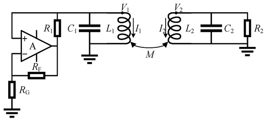
Figure 1.
Block diagram of the circuit of a typical nonlinear parity-time-symmetric wireless power (NPTS-WPT) system.
According to Kirchhoff’s laws, we have
where j is the imaginary unit, ω is the operating angular frequency of the system, and A is the amplification factor of the OP Amp, which is (RF + RG)/RG in the linear region.
Let ω1 and ω2 be the natural resonant angular frequencies of the Tx and Rx loops, respectively: , . For a completely matched NPTS-WPT system, ω1 = ω2 [4,14,15]. However, when the system is detuned, ω1 ≠ ω2.
The coupling coefficient of the two coils is .
Let
where γ1 is the gain rate of the Tx circuit, and γ2 is the loss rate in the Rx circuit [14].
Equation (1) can then be reduced to the following matrix form:
If Equation (4) has a solution, the determinant of the coefficient matrix must be 0, resulting in Equation (5):
Let ω be a real number; the real and imaginary parts of Equation (5) must simultaneously be 0—namely,
To represent the inconsistency between the natural resonant angular frequency at the Rx end and that at the Tx end, we define the degree of detuning of the system as follows:
Given that too much detuning is of little practical value, this paper set the following restriction for αω:
From Equations (6) and (7), Equation (10) can be derived:
Equation (10) can be considered as a cubic equation of the variable (ω/ω1)2 and can be solved based on Shengjin’s formula [28]. Please refer to the Appendix A as Equations (A1)–(A3) for solution details, where Δ and AS are the general discriminant and the first discriminant of Equation (10), which will be frequently mentioned in the following analysis.
The NPTS-WPT system can select an appropriate amplification factor (A) for the OP Amp based on the actual operation of the system to maintain the resonant state [4]. When the system is detuned, the A of the OP Amp of the system can be obtained from Equations (2), (6) and (8):
For a WPT system, the transfer efficiency is an important indicator. In this paper, we consider only the transfer efficiency—i.e., the efficiency from the Tx coil to the load resistor at the Rx end. In the above analysis, for simplicity, the ideal circuit is mathematically modeled. Under ideal conditions, the inductors and capacitors are energy storage and transducer devices and do not consume any energy. In practical scenarios, the intrinsic resistance of a capacitor can be neglected, but the intrinsic resistance of an inductor cannot be ignored. To further consider the transfer efficiency of the system, we will consider the intrinsic resistance of the inductor. Thus, the transfer efficiency of the system is defined by Equation (12)
where RL1 and RL2 are the inherent resistances of the Tx and Rx coils, respectively, and the final formula is shown in Equation (13).
3. Analysis of the Transfer Characteristics at Complete Matching
To analyze the dependence of the transfer characteristics of a system on the distance between the Tx and Rx coils, the dependence of the coupling coefficient between the coils on the distance between them was plotted using the experimentally obtained data, as shown in Figure 2.
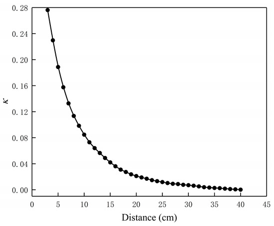
Figure 2.
Coupling coefficient between the Tx and Rx coils versus the distance between them plotted using the experimentally obtained data.
The circuit parameters extracted from the experimental system are substituted into Equations (A4)–(A9) as it is seen in Appendix A. Then, let αω = 1, and the dependence of the operating frequency of the system on the distance between the Tx and Rx coils at complete matching can be obtained, as shown by the black curve in Figure 3. The figure shows that when Δ < 0, there are three frequency branches in the system. According to the relative magnitude of the operating frequency, these branches are called the high-frequency branch, the mid-frequency branch and the low-frequency branch. Moreover, although the mid-frequency branch of the system theoretically exists when Δ < 0, it cannot be observed in the experiment due to its instability. Therefore, a black dotted line is used in Figure 3 to represent the mid-frequency branch. When Δ > 0, there is only one frequency branch in the system.
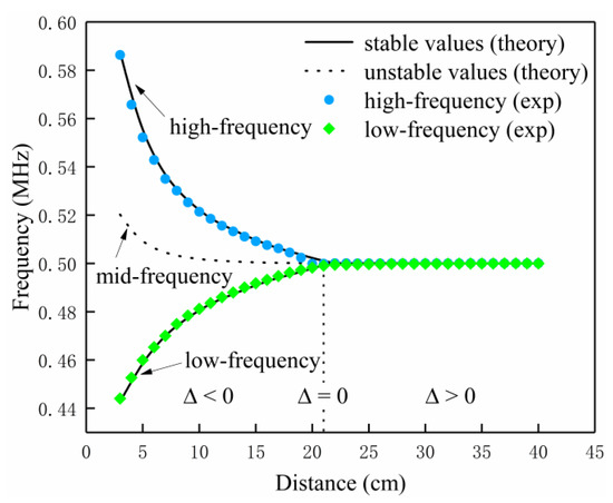
Figure 3.
Operating frequency versus distance between the Tx and Rx coils at complete matching.
When Δ = 0, there are one or two operating frequencies in the system, depending on the value of AS. When AS = 0, there is only one operating frequency in the system, and if two coils pass through this position in the process of gradually moving away, the three frequency branches will converge here, as shown in Figure 4. When AS ≠ 0, there are two frequencies in the system, so two of the three frequency branches will converge in this situation. Because there is only one frequency branch in the system when Δ > 0, if the two coils pass through the position gradually, the operating frequency will change suddenly. For example, at Δ = 0, the low-frequency branch and the mid-frequency branch of the system converge, and when the distance between the two coils further increases, the high-frequency branch of the system will suddenly disappear, leaving only the converged branch, as shown in Figure 5. Thus, even in the case of complete matching, a frequency jump may occur in the system.
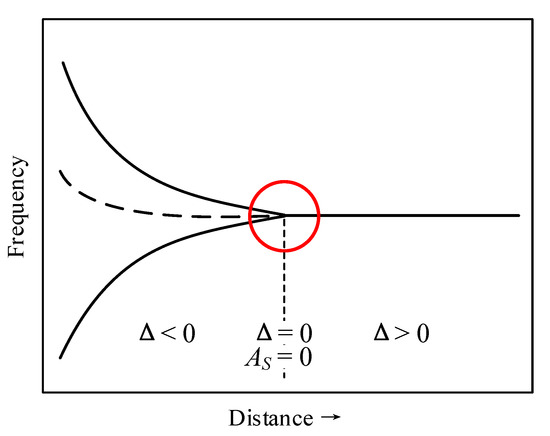
Figure 4.
Operating frequency versus distance between the Tx and Rx coils at complete matching (when Δ = 0, AS = 0).
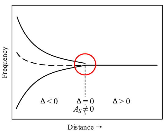
Figure 5.
Operating frequency versus distance between the Tx and Rx coils at complete matching (when Δ = 0, AS ≠ 0).
By substituting the corresponding parameters into Equation (11), the amplification factor A of the different frequency branches at different distances can be obtained, as shown in Figure 6. The figure shows that the high-frequency and low-frequency branches have the same A, while the A values of the unstable mid-frequency branch are higher than those of the high- frequency and low-frequency branches. The difference between the A values of the mid-frequency branch and those of the other two branches becomes more prominent as the distance between the coils decreases. Therefore, it can be seen that the system preferentially selects frequency branches with lower A values.
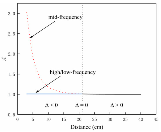
Figure 6.
Amplification factor for different frequency branches versus the distance between the Tx and Rx coils at complete matching.
To further analyze the dependence of A on the distance, the corresponding A of the mid-frequency branch were discarded, and the curve was replotted as shown in Figure 7. The figure shows that when Δ < 0, A basically remains the same; when Δ approaches 0, A starts to gradually decrease; and when Δ > 0, A further decreases. It is worth noting that regardless of how A decreases, its value is always greater than 1.
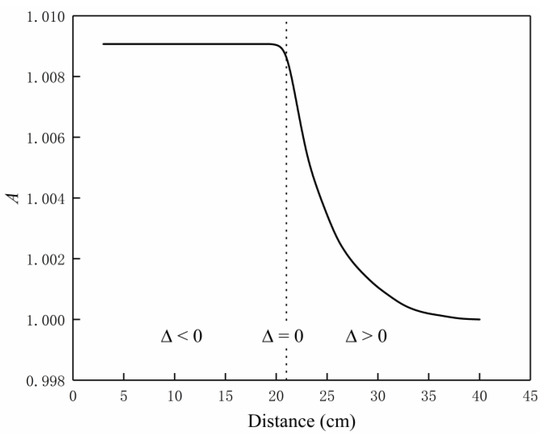
Figure 7.
Amplification factor versus the distance between the Tx and Rx coils at complete matching (the actual values adopted by the system).
4. Analysis of Transfer Characteristics at Detuning
When αω ≠ 1, the system is detuned. The detuning in this paper is classified into two types: under-detuning and over-detuning. For the high-frequency branch, under-detuning refers to the stage with αω < 1, and over-detuning refers to the stage with αω > 1. For the low-frequency branch, under-detuning refers to αω > 1, and over-detuning refers to αω < 1.
Due to the complex characteristics of operating frequency and transfer efficiency of the system when Δ < 0, this paper focuses on the characteristics of detuning when Δ < 0. For comparison, the coupling coefficients κ of 0.11, 0.073, and 0.049 were chosen for three scenarios, and the corresponding distances are 8, 11, and 14 cm. By substituting the relevant parameters into Equations (A4)–(A9), the dependence of the operating frequency of the system on αω can be plotted, as shown by the solid lines in Figure 8. The unstable mid-frequency branch is not considered here.
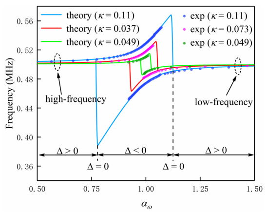
Figure 8.
Operating frequency of the system versus αω at detuning.
Taking κ = 0.11 as an example, the high-frequency branch of the system initiates from the left side of Figure 8. When αω increases, the operating frequency gradually increases. When αω = 1, the system reaches complete resonance, and when αω further increases, the operating frequency further increases. However, when Δ = 0, the high-frequency branch disappears, and the operating frequency jumps to the low-frequency branch. When αω continues to increase, the operating frequency slowly increases on the low-frequency branch. The low-frequency branch of the system is similar to the high-frequency branch.
The figure also shows that two dotted lines (corresponding to Δ = 0) divide the entire region (0.5 ≤ αω ≤ 1.5) into three subregions. Δ is less than zero in the middle region, and the system has two frequency branches (does not consider the unstable mid-frequency branch) in this region. Δ is greater than zero in the two side regions, and the system has only one frequency branch in these regions; the side region on the left has only a high-frequency branch, while the side region on the right has only a low-frequency branch.
Moreover, from the comparison of the three curves for κ values of 0.11, 0.073, and 0.049, it can be seen that as κ decreases, the point at which the frequency jumps keeps advancing.
Next, the amplification factor A of the OP Amp was used to explain the reason for the jump in the operating frequency of the system, as shown in Figure 9. Taking κ = 0.11 as an example, along the arrow in the figure, when αω decreases from 1.5, A gradually increases along the solid blue line. When A reaches the low-frequency-to-high-frequency (LTH) point, A cannot increase further, since there is no higher A value on the low-frequency branch as αω continues to decrease. Therefore, the A value of the system drops along the arrow to the branch on the left side, i.e., the operating frequency of the system jumps from the low-frequency branch to the high-frequency branch, where the LTH point corresponds to Δ = 0. Similarly, if αω starts to move from the left side to the right side, A will jump at the high-frequency-to-low-frequency (HTL) point, i.e., the operating frequency of the system jumps from the high-frequency branch to the low-frequency branch.
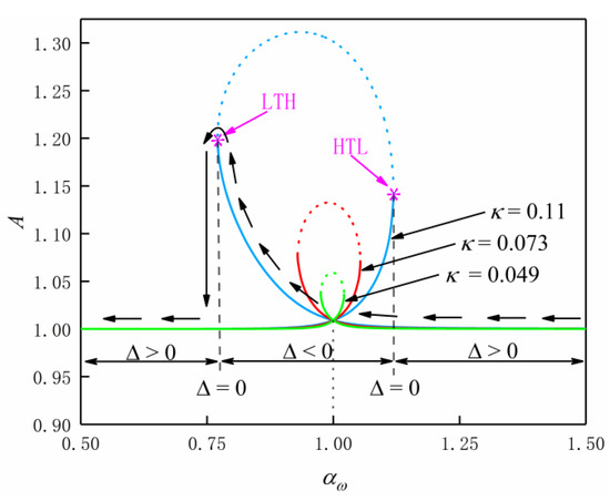
Figure 9.
Amplification factor of the operational amplifier (OP) Amp versus αω at detuning.
In Figure 9, there is a dotted curve in the middle of each curve. Each dotted curve corresponds to the unstable mid-frequency branch. The figure shows that the A values of the dotted curves are much larger than the A values of the solid curves. The system selects the state corresponding to a smaller A value and stabilizes. In the region with Δ < 0, the OP Amp has two stable A values. Although the system prefers the smaller A, in the absence of external disturbance, the system will follow the previous trajectory (similar to inertia), even if the system has the option to choose a smaller A value.
Moreover, from the comparison of the three curves for κ values of 0.11, 0.073, and 0.049, the A required for under-detuning decreases as κ decreases for both the high-frequency branch and the low-frequency branch, and the A required for over-detuning increases as κ decreases. It is worth noting that, as shown in the figure, when αω = 1, the high-frequency branches and the low-frequency branches for the different κ values intersect at the same point, which means the system always requires the same A for complete matching.
Next, the dependence of ƞ on αω was investigated. The figure shows the ƞ values of the high-frequency and low-frequency branches corresponding to the three κ values of 0.11, 0.073, and 0.049. On the ƞ curves corresponding to the high-frequency branches, ƞ increases with αω. More specifically, the growth of ƞ was rapid at under-detuning and was slow at over-detuning. On the ƞ curves corresponding to the low-frequency branches, ƞ decreases with αω. More specifically, the growth of ƞ was rapid at under-detuning and was slow at over-detuning.
It can be seen from Figure 10 that when the detuning factor is fixed, the transfer efficiency decreases with the increase in distance for the under-detuning stage and increases with the increase in distance for the over-detuning stage. However, due to the frequency jump, the transfer efficiency does not increase continuously, because a further increase in distance will make the system jump to the under-detuning stage.
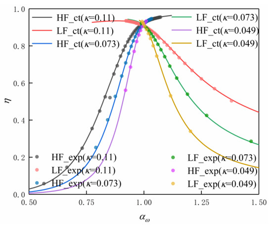
Figure 10.
Transfer efficiency versus αω at detuning where HF_ct, LF_ct, HF_exp and LF_exp mean theoretical high-frequency, theoretical low-frequency, experimental high-frequency and experimental low-frequency, respectively.
The system is completely matched when αω = 1, and it can be seen from Figure 10 that when the system is over-coupled, the transfer efficiency is higher than that when the system is completely matched. Thus, we can see that for an NPTS-WPT system that satisfies Δ < 0, detuning does not mean reduced transfer efficiency. If the system is maintained in an over-detuning mode, the transfer efficiency will be higher than the transfer efficiency at complete matching.
5. Experimental Verification
5.1. Experimental Setup
To verify the validity of the above theory, a prototype was constructed, and the experimental system is shown in Figure 11. The experimental system consists of an LCR tester, an oscilloscope, a DC voltage source, and an NPTS-WPT system. The NPTS-WPT system consists of a Tx circuit, a Tx coil, an Rx coil and an Rx circuit. The LCR tester was mainly used to test the coupling coefficient between the Tx and Rx coils and the natural resonant frequencies of the Tx and Rx loops. The oscilloscope was mainly used to collect the waveforms of the voltages across the Tx and Rx coils and to calculate the operating frequency and voltage amplitude in real time. The DC voltage source was used to power the NPTS-WPT system. The relevant parameters of the experimental system are listed in Table 1. In addition, the system uses a general-purpose OP Amp LM7171, and the peripheral resistances are RF = 510 Ω and RG = 5.1 kΩ.
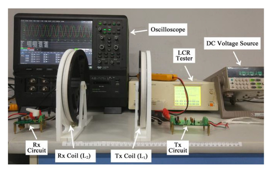
Figure 11.
Experimental setup.

Table 1.
Experiment parameters of the system.
5.2. Verification of the Trasfer Characteristics at Complete Matching
The matching capacitors at the Tx and Rx ends were adjusted so that the natural resonant frequencies of the Tx and Rx loops reached 0.5 MHz, and the system was at complete matching. The position of the Rx coil was fixed, and the position of the Tx coil was adjusted so that the distance between the two coils was changed from 3 to 40 cm, at a step length of 1 cm. The operating frequency solved in real-time on the oscilloscope was recorded, and the dependence of the operating frequency on distance was plotted, as shown by the scattered points in Figure 3. The blue dots represent the dependence of the actual operating frequency on distance when the system is in the high-frequency branch, and the green diamonds represent the dependence of the actual operating frequency on distance when the system is in the low-frequency branch.
The figure shows that when Δ < 0, the system has two frequency branches (high-frequency branch and low-frequency branch). It should be noted that in an actual system, the mid-frequency branch is unstable due to the extremely high amplification factor; therefore, the mid-frequency branch will not appear in the experimental system. Convergence occurs when Δ = 0. When Δ > 0, the system has only one frequency branch. Our experimental system satisfies AS ≠ 1 at the convergence point, and its operating frequency jumps at the convergence point. This phenomenon is observed in the experiment, but it cannot be reflected in the figure because it appears between two continuous measurements. By comparing the solid curves and the scattered points in the figure, we can see that the experimental results are basically in agreement with the theoretical calculations, but the distance corresponding to the frequency convergence point of the experimental results is slightly shorter than the distance corresponding to the theoretically calculated frequency convergence point. This result occurs mainly because the theoretical model did not consider the intrinsic resistance of the coils (parasitic effects, including parasitic capacitance and parasitic inductance, were neglected, since the system frequency was low). In theoretical modeling, the intrinsic resistance of the coils is not considered, greatly simplifying the mathematical model-solving process without having a large impact on the results, so this simplification is acceptable.
5.3. Verification of the Trasfer Characteristics at Detuning
The distance between the fixed Tx coil and the Rx coil is 8 cm. At detuning, the operating frequency characteristics of the system must be tested separately for the two frequency branches. For the high-frequency branch, the capacitor at the Rx end was adjusted so that the operating frequency of the system was 503 kHz. The matching capacitor was separated from the Rx loop, and then the capacitance of the capacitor at the corresponding frequency was measured using the LCR tester. The natural resonant frequency of the Rx loop was calculated using the capacitance and inductance of the Rx coil, and then, αω was calculated. Next, the operating frequency of the system was continuously increased at a step length of 1 kHz, and the above operation was repeated until the system could not maintain its high-frequency branch. For the low-frequency branch, we used a similar method to reduce the operating frequency of the system from 497 kHz at a step length of 1 kHz until the system could not maintain the low-frequency branch. For comparison, we repeated the above experiment when the distance between the Tx and Rx coils was 11 and 14 cm. Using the above method, the dependence of the operating frequency of the system on αω was plotted, as shown by the scatterplots in Figure 8. As long as the amplitudes of the voltages across the coils were simultaneously measured in the above experiment, the dependence of the ƞ on αω could be plotted, as shown by the scatterplots in Figure 10, where we can see that the experimental results are basically in agreement with the theoretical calculations.
The comparison of the experimental results and the theoretical calculations in Figure 8 shows that although the trend of the experimental results is consistent with the trend of the theoretical calculation (experimentally measured datapoints are basically on the theoretically calculated curve), the experimental jump point comes much earlier than the theoretical jump point, not only because of the neglect of the intrinsic resistance of the coils in the theoretical calculation but also because of the unsatisfactory amplification performance of the actual OP Amp. The actual operation cannot provide a sufficiently large amplification factor (theoretically required), and the vibration caused by the experimental operation triggers the early occurrence of the sensitive jumping point.
6. Conclusions
This paper focuses on the transfer characteristics of the NPTS-WPT system at detuning between the Tx and Rx. A system circuit model is established. Based on the circuit theory, an accurate analytical solution for the operating frequency, the amplification factor of the operational amplifier and the transfer efficiency at detuning is derived, and the correctness of the theory is validated through the established experimental system.
The general discriminant of the system state is defined as Δ. When Δ < 0, there are three frequency branches in the system: a high-frequency branch, a low-frequency branch and a mid-frequency branch (because of instability, the mid-frequency branch was not observed in the experiment). When Δ = 0, these three frequency branches converge (three branches converge at the same time, or only two branches converge). When Δ > 0, the system has only one frequency branch. For a completely matched system, when Δ < 0 the system maintains a high transfer efficiency, and when Δ ≥ 0, the transfer efficiency of the system gradually decreases as the distance between Tx and Rx increases.
For the system at detuning, two detuning modes are defined: under-detuning and over-detuning. Under-detuning will reduce the transfer efficiency, while over-detuning can improve the transfer efficiency to a certain extent.
This paper is the first to note that even if the Tx and Rx are completely matched, a frequency jump might occur when the distance between them changes slowly. It has been found that when the degree of detuning changes, the operating frequency of the system will jump. By investigating the amplification factor of the operational amplifier, we preliminarily explained the reason for the frequency jump when the system was detuned. The nonlinear dynamic characteristics of the NPTS-WPT system should be studied to provide further explanations, and we are trying to explore this aspect. The results obtained by this paper are a supplement to the transfer characteristics of the NPTS-WPT system and will improve the popularity of the system in wireless power transfer with variable gap, such as mobile robot charging, electric vehicle charging, and spring chain power supply.
Author Contributions
C.L. and W.D. contributed equally to this work. Conceptualization, C.L.; Methodology, C.L., W.D., L.D.; Validation, C.L., W.D., L.D., H.Z., H.S.; Formal analysis, W.D., C.L.; Investigation, C.L., W.D., H.S.; C.L. and W.D., writing—original draft preparation, and writing—review and editing; Visualization, W.D.; funding acquisition, H.Z. All authors have read and agreed to the published version of the manuscript.
Funding
This work was supported in part by the National Natural Science Foundation of China under Grant 61403201, in part by the Advanced Research Project of the 13th Five-Year Plan under Grant 41419050104, in part by the Six Talent Peak Projects under Grant KTHY-019, and in part by the National Key Laboratory Foundation under Grant 6142601180101.
Conflicts of Interest
The authors declare no conflict of interest.
Appendix A
Solution of operating angular frequencies
Before solving (10), define a, b, c and d as follows:
and let
where AS, BS and CS are called the first, second and third discriminant, respectively.
The general discriminant of (10) is then
According to Shengjin’s formula, (10) has the following solutions (only positive real solutions are considered):
- If Δ < 0, there are three different real rootswhere
- If Δ = 0, and AS ≠ 0, there are three real roots, two of which are equal:
- If Δ = 0 and AS = 0, there is a real triple root:
- If Δ > 0, there is a real root and a pair of complex conjugate roots. The real root can be expressed as (A5)where
It should be noted that the above formulas solve the operating angular frequency, but the oscilloscope measures the operating frequency. Dividing the angular frequency by 2 π is the operating frequency in the paper.
References
- Kim, J.; Kim, H.; Kim, D.; Park, H.-J.; Ban, K.; Ahn, S.; Park, S.-M. A wireless power transfer based implantable ECG monitoring device. Energies 2020, 13, 905. [Google Scholar] [CrossRef]
- Wang, Y.; Song, B.; Mao, Z. Analysis and experiment for wireless power transfer systems with two kinds shielding coils in EVs. Energies 2020, 13, 277. [Google Scholar] [CrossRef]
- Maier, D.; Parspour, N. Wireless charging—A multi coil system for different ground clearances. IEEE Access 2019, 7, 123061–123068. [Google Scholar] [CrossRef]
- Assawaworrarit, S.; Yu, X.; Fan, S. Robust wireless power transfer using a nonlinear parity–time-symmetric circuit. Nature 2017, 546, 387–390. [Google Scholar] [CrossRef] [PubMed]
- Fang, Y.; Wang, Y.; Xia, J. Large-range electric field sensor based on parity-time symmetry cavity structure. Chin. J. Phys. 2019, 68, 92–100. [Google Scholar] [CrossRef]
- Cao, T.; Cao, Y.; Fang, L. Reconfigurable parity-time symmetry transition in phase change metamaterials. Nanoscale 2019, 11, 15828–15835. [Google Scholar] [CrossRef]
- Bender, C.M.; Hassanpour, N.; Klevansky, S.P.; Sarkar, S. PT-symmetric quantum field theory in D dimensions. Phys. Rev. D 2018, 98. [Google Scholar] [CrossRef]
- Schindler, J.; Lin, Z.; Lee, J.M.; Ramezani, H.; Ellis, F.M.; Kottos, T. PT-symmetric electronics. J. Phys. A Math. Theor. 2012, 45, 444029. [Google Scholar] [CrossRef]
- Peng, B.; Özdemir, Ş.K.; Lei, F.; Monifi, F.; Gianfreda, M.; Long, G.L.; Fan, S.; Nori, F.; Bender, C.M.; Yang, L. Parity–time-symmetric whispering-gallery microcavities. Nat. Phys. 2014, 10, 394–398. [Google Scholar] [CrossRef]
- Beygi, A.; Klevansky, S.P.; Bender, C.M. Coupled oscillator systems having partialPTsymmetry. Phys. Rev. A 2015, 91. [Google Scholar] [CrossRef]
- Yang, J. Nonlinear behaviors in a PDE model for parity-time-symmetric lasers. J. Opt. 2017, 19, 054004. [Google Scholar] [CrossRef]
- Li, J.; Zhan, X.; Ding, C.; Zhang, D.; Wu, Y. Enhanced nonlinear optics in coupled optical microcavities with an unbroken and broken parity-time symmetry. Phys. Rev. A 2015, 92. [Google Scholar] [CrossRef]
- Feng, L.; Wong, Z.J.; Ma, R.-M.; Wang, Y.; Zhang, X. Single-mode laser by parity-time symmetry breaking. Science 2014, 346, 972–975. [Google Scholar] [CrossRef] [PubMed]
- Dong, W.; Zhang, H.; Li, C.; Liao, X. Research on variable gap wireless energy transmission method for fuzes based on nonlinear PT symmetry principle. Acta Armamentarii 2019, 40, 35–41. [Google Scholar]
- Dong, W.; Li, C.; Zhang, H.; Ding, L. Wireless power transfer based on current non-linear PT-symmetry principle. IET Power Electron. 2019, 12, 1783–1791. [Google Scholar] [CrossRef]
- Shu, X.; Zhang, B. Single-wire electric-field coupling power transmission using nonlinear parity-time-symmetric model with coupled-mode theory. Energies 2018, 11, 532. [Google Scholar] [CrossRef]
- Zhou, J.; Zhang, B.; Xiao, W.; Qiu, D.; Chen, Y. Nonlinear parity-time-symmetric model for constant efficiency wireless power transfer: Application to a drone-in-flight wireless charging platform. IEEE Trans. Ind. Electron. 2019, 66, 4097–4107. [Google Scholar] [CrossRef]
- Liu, G.; Zhang, B. Dual-coupled robust wireless power transferbased on parity-time-symmetric model. Chin. J. Electr. Eng. 2018, 4, 50–55. [Google Scholar]
- Ra’Di, Y.; Chowkwale, B.; Valagiannopoulos, C.; Liu, F.; Alu, A.; Simovski, C.R.; Tretyakov, S.A. On-site wireless power generation. IEEE Trans. Antennas Propag. 2018, 66, 4260–4268. [Google Scholar] [CrossRef]
- Liu, F.; Chowkwale, B.; Jayathurathnage, P.; Tretyakov, S. Pulsed self-oscillating nonlinear systems for robust wireless power transfer. Phys. Rev. Appl. 2019, 12. [Google Scholar] [CrossRef]
- Pantic, Z.; Lukic, S.M. Framework and topology for active tuning of parallel compensated receivers in power transfer systems. IEEE Trans. Power Electron. 2012, 27, 4503–4513. [Google Scholar] [CrossRef]
- Lu, J.; Zhu, G.; Wang, H.; Lu, F.; Jiang, J.; Mi, C.C. Sensitivity analysis of inductive power transfer systems with voltage-fed compensation topologies. IEEE Trans. Veh. Technol. 2019, 68, 4502–4513. [Google Scholar] [CrossRef]
- Fu, W.; Zhang, B.; Qiu, D. Study on frequency-tracking wireless power transfer system by resonant coupling. In Proceedings of the 2009 IEEE 6th International Power Electronics and Motion Control Conference (IPEMC 2009), Wuhan, China, 17–20 May 2009. [Google Scholar]
- Cao, J.; Zhang, H.; Wang, X.; Miao, D. Influence of load impedance characteristics on transmission performance of fuze wireless setting system based on magnetic resonance coupling. Acta Armamentarii 2018, 39, 2330–2337. [Google Scholar]
- Mai, R.; Liu, Y.; Li, Y.; Yue, P.; Cao, G.; He, Z. An active-rectifier-based maximum efficiency tracking method using an additional measurement coil for wireless power transfer. IEEE Trans. Power Electron. 2018, 33, 716–728. [Google Scholar] [CrossRef]
- Feng, H.; Cai, T.; Duan, S.; Zhang, X.; Hu, H.; Niu, J. A dual-side-detuned series–series compensated resonant converter for wide charging region in a wireless power transfer system. IEEE Trans. Ind. Electron. 2018, 65, 2177–2188. [Google Scholar] [CrossRef]
- Ren, J.; Yang, D.; Liu, D.; Hu, P. Tuning of mid-range wireless power transfer system based on delay-iteration method. IET Power Electron. 2016, 9, 1563–1570. [Google Scholar] [CrossRef]
- Liu, H.; Liu, Q.; Zhou, S.; Li, C.; Yuan, S. A NURBS interpolation method with minimal feedrate fluctuation for CNC machine tools. Int. J. Adv. Manuf. Technol. 2015, 78, 1241–1250. [Google Scholar] [CrossRef]


© 2020 by the authors. Licensee MDPI, Basel, Switzerland. This article is an open access article distributed under the terms and conditions of the Creative Commons Attribution (CC BY) license (http://creativecommons.org/licenses/by/4.0/).