Power, Efficiency, Power Density and Ecological Function Optimization for an Irreversible Modified Closed Variable-Temperature Reservoir Regenerative Brayton Cycle with One Isothermal Heating Process


Abstract
1. Introduction
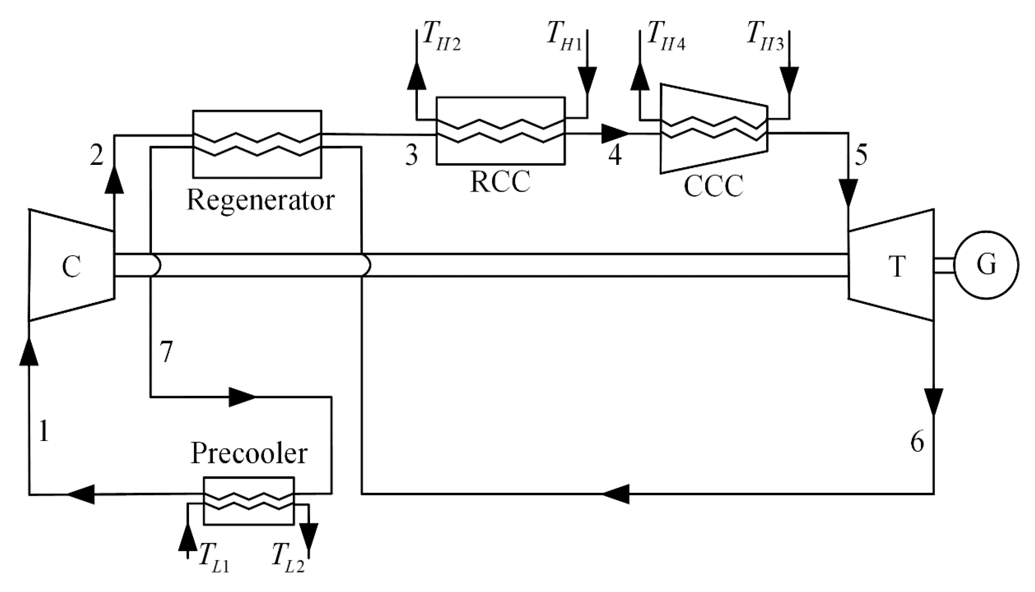
2. Cycle Model
3. Single Objective Analysis and Optimization
3.1. Single Objective Analysis
3.2. Single Objective Optimization
3.2.1. Optimal Distributions of Heat Exchanger Inventory
3.2.2. Optimal Thermal Capacitance Rate Matching among the WF and Heat Reservoir
4. Multi-Objective Optimization
5. Conclusions
- (1)
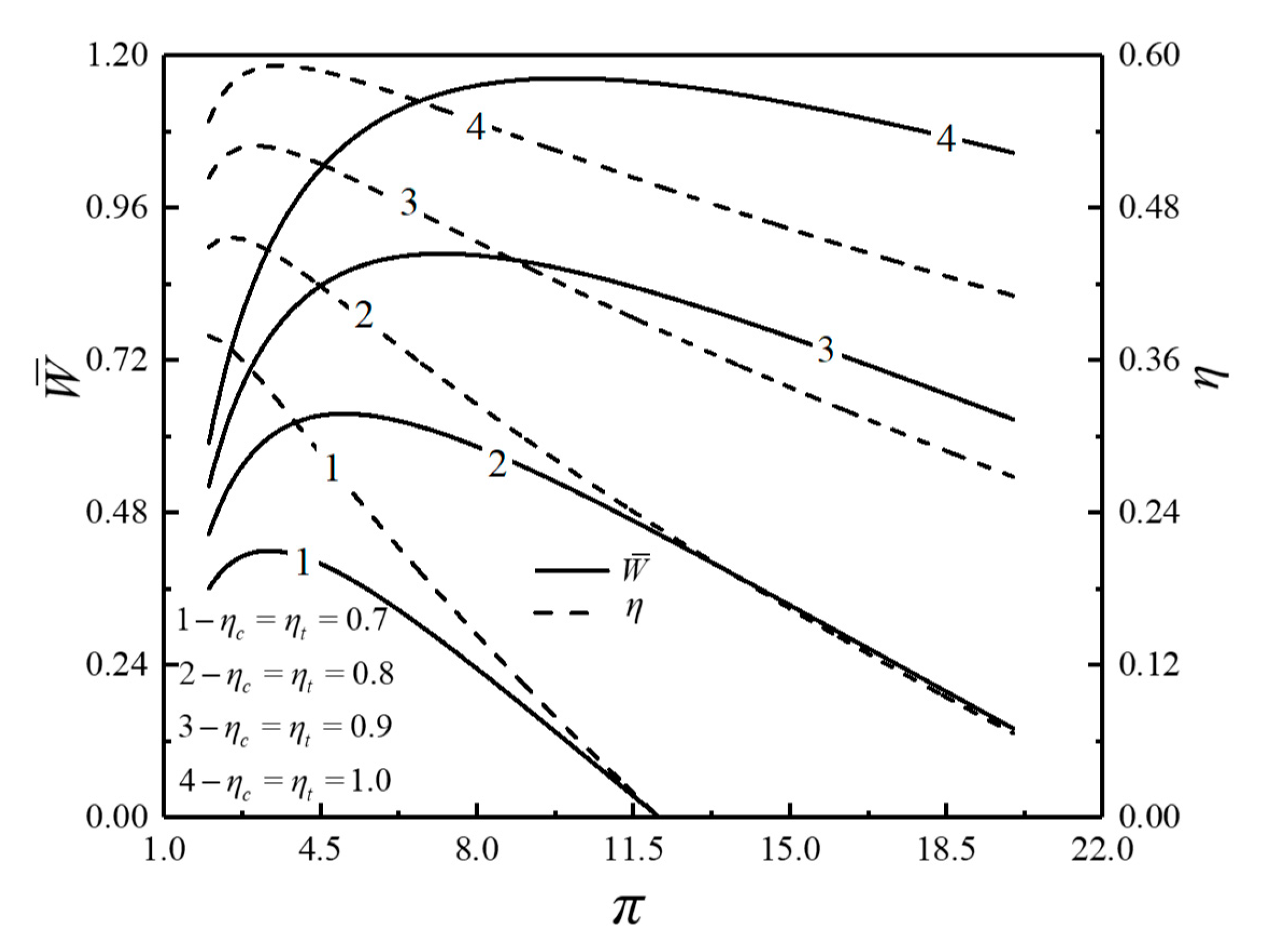
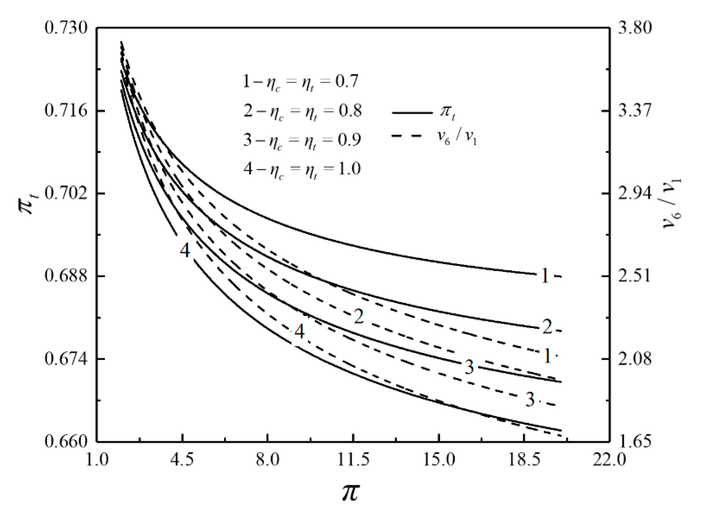
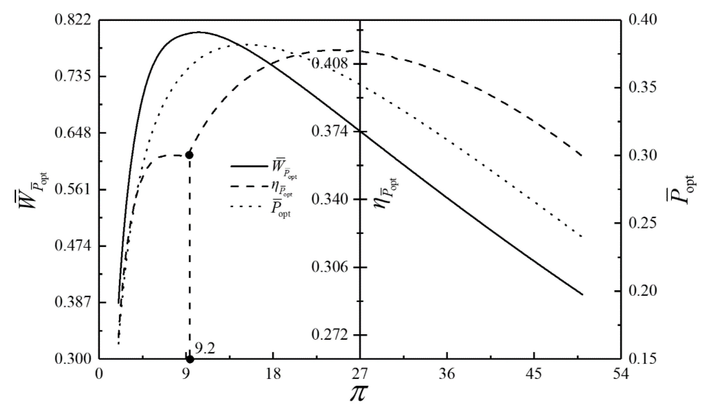
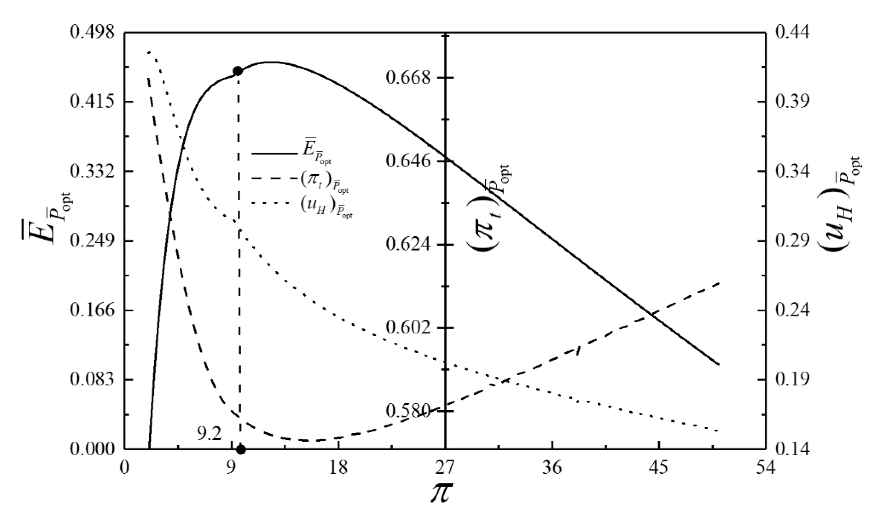
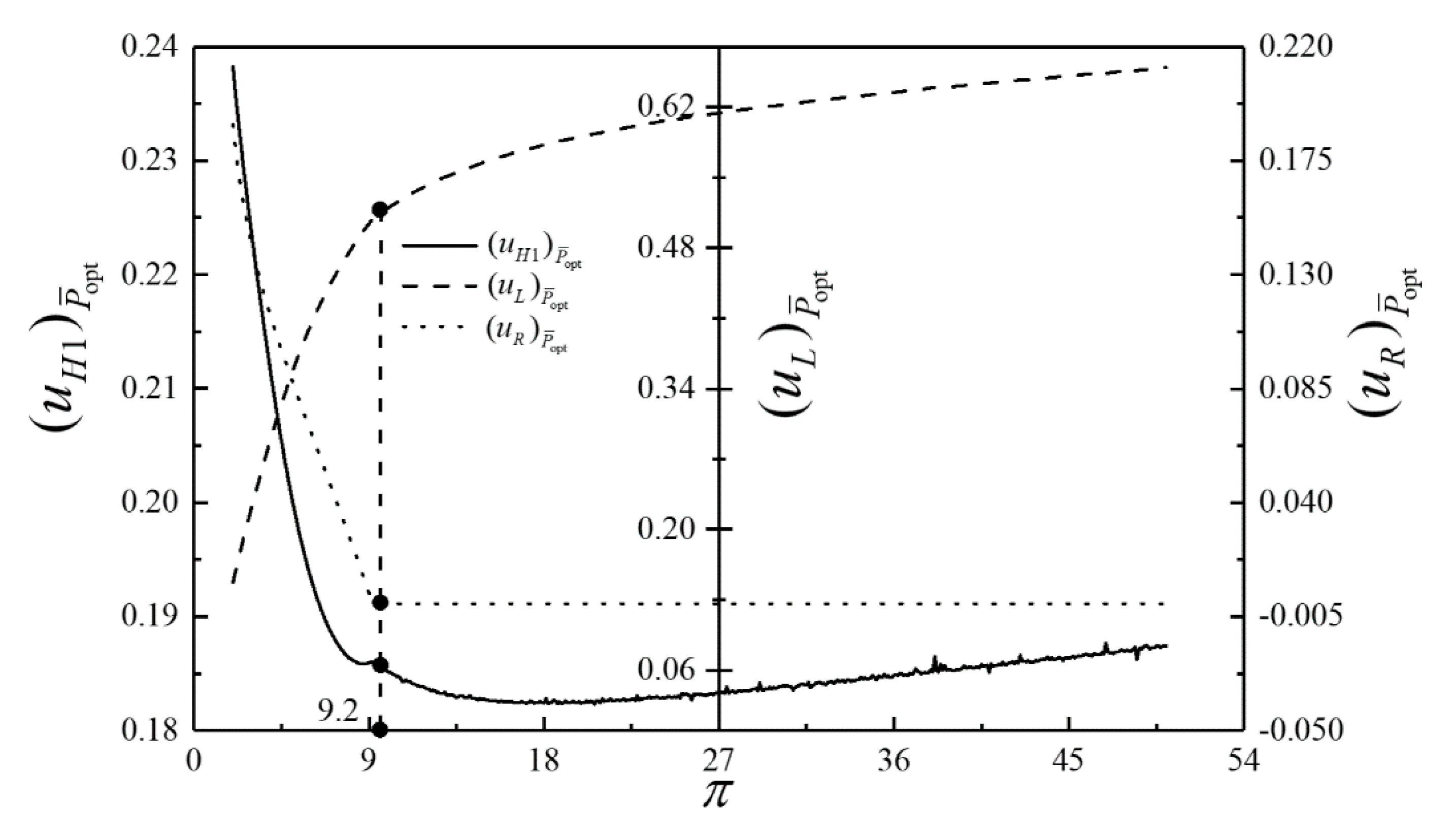
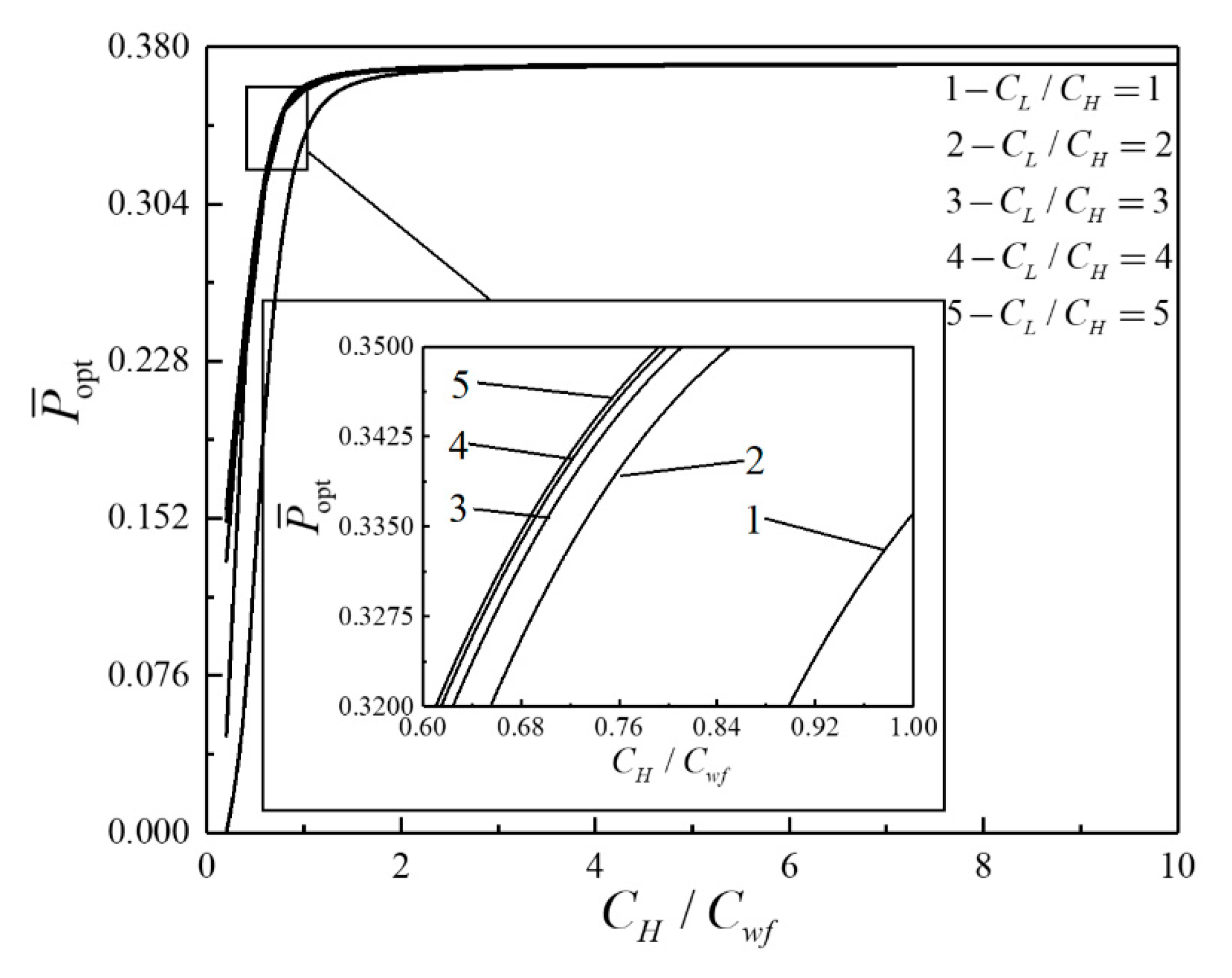
- For the single objective analysis, the DPO, TEF, DPD and DEF all augment first and then reduce as augments. When , it is beneficial to add the regenerator to improve the cycle performance; when , adding the regenerator will reduce the cycle performance. For the single-objective optimization, when , the effectiveness at the regenerator should be 0, and the cycle will be simplified into a closed irreversible modified BCY with an IHP and coupled to VTHRs. Hence, the regenerator is added, and a suitable pressure ratio should be selected in the limited range. In the actual process, the pressure ratio should be strictly controlled in this new-type gas turbine, or the new-type gas turbine is suitable for the situations where the pressure ratio is relatively low. The DPO, TEF, DPD and DEF increase as or increases. and decrease as or increases. It indicates that the cycle performance and the degree of the cycle’s isothermal heating correction are improved and the volume of the cycle device is reduced by reducing the irreversibility of the cycle.
- (2)
- For the quadruple objective optimization, the results gained by LINMAP and TOPSIS methods are the same, and D is smaller than that gained by the Shannon entropy method. Therefore, the results gained by LINMAP and TOPSIS methods are better than those gained by the Shannon entropy method. For the double, triple or quadruple objective optimization, the triple objective (, and ) optimization’ deviation index gained by LINMAP or TOPSIS method is the smallest. According to decision-makers’ actual needs, they could choose the best scheme from the Pareto frontier, design the new-type gas turbine reasonably, and then determine the construction or the operation of the gas turbine.
Author Contributions
Funding
Acknowledgments
Conflicts of Interest
Nomenclature
| C | Thermal capacitance rate (kW/K) |
| E | Effectiveness, ecological function (kW/K) |
| Dimensionless ecological function | |
| Dimensionless power density | |
| T | Temperature (K) |
| U | Heat conductance (kW/K) |
| u | Heat conductance distribution |
| Dimensionless power output | |
| Greek symbol | |
| Efficiency | |
| Pressure ratio | |
| Temperature ratio | |
| Subscripts | |
| H | Heat exchanger at the regular combustion chamber |
| H1 | Heat exchanger at the converging combustion chamber |
| L | Cold-side heat exchanger at the precooler |
| wf | Working fluid |
| 1-7,2s,6s | State points |
Abbreviations
| BCY | Brayton cycle |
| CCC | Converging combustion chamber |
| CTHR | Constant-temperature heat reservoir |
| DEF | Dimensionless ecological function |
| DPD | Dimensionless power density |
| DPO | Dimensionless power output |
| FTT | Finite-time thermodynamics |
| HCD | Heat conductance distribution |
| IHP | Isothermal heating process |
| IPDR | Isothermal pressure drop ratio |
| NIP | Negative ideal point |
| PIP | Positive ideal point |
| RCC | Regular combustion chamber |
| TEF | Thermal efficiency |
| VTHR | Variable-temperature heat reservoir |
| WF | Working fluid |
References
- Vecchiarelli, J.; Kawall, J.G.; Wallace, J.S. Analysis of a concept for increasing the efficiency of a Brayton cycle via isothermal heat addition. Int. J. Energy Res. 1997, 21, 113–127. [Google Scholar] [CrossRef]
- Göktun, S.; Yavuz, H. Thermal efficiency of a regenerative Brayton cycle with isothermal heat addition. Energy Convers. Manag. 1999, 40, 1259–1266. [Google Scholar] [CrossRef]
- Erbay, L.B.; Göktun, S.; Yavuz, H. Optimal design of the regenerative gas turbine engine with isothermal heat addition. Appl. Energy 2001, 68, 249–264. [Google Scholar] [CrossRef]
- Jubeh, N.M. Exergy analysis and second law efficiency of a regenerative Brayton cycle with isothermal heat addition. Entropy 2005, 7, 172–187. [Google Scholar] [CrossRef]
- El-Maksound, R.M.A. Binary Brayton cycle with two isothermal processes. Energy Convers. Manag. 2013, 73, 303–308. [Google Scholar] [CrossRef]
- Andresen, B.; Salamon, P.; Berry, R.S. Thermodynamics in finite time. Phys. Today 1987, 37, 62–70. [Google Scholar] [CrossRef]
- Berry, R.S.; Kazakov, V.A.; Sieniutycz, S.; Szwast, Z.; Tsirlin, A.M. Thermodynamic Optimization of Finite Time Processes; Wiley: Chichester, UK, 1999. [Google Scholar]
- Dincer, I.; Zamfirescu, C. Advanced Power Generation Systems; Elsevier: London, UK, 2014. [Google Scholar]
- Perescu, S.; Costea, M.; Feidt, M.; Ganea, I.; Boriaru, N. Advanced Thermodynamics of Irreversible Processes with Finite Speed and Finite Dimensions; Editura AGIR: Bucharest, Romania, 2015. [Google Scholar]
- Kaushik, S.C.; Tyagi, S.K.; Kumar, P. Finite Time Thermodynamics of Power and Refrigeration Cycles; Springer: New York, NY, USA, 2018. [Google Scholar]
- Sieniutycz, S. Complexity and Complex Thermo-Economic Systems; Elsevier: Amsterdam, The Netherlands, 2020. [Google Scholar]
- Chen, L.G.; Wu, C.; Sun, F.R. Finite time thermodynamic optimization or entropy generation minimization of energy systems. J. Non-Equilib. Thermodyn. 1999, 24, 327–359. [Google Scholar] [CrossRef]
- Andresen, B. Current trends in finite-time thermodynamics. Angew. Chem. Int. Edition. 2011, 50, 2690–2704. [Google Scholar] [CrossRef]
- Roach, T.N.F.; Salamon, P.; Nulton, J.; Andresen, B.; Felts, B.; Haas, A.; Calhoun, S.; Robinett, N.; Rohwer, F. Application of finite-time and control thermodynamics to biological processes at multiple scales. J. Non-Equilib. Thermodyn. 2018, 43, 193–210. [Google Scholar] [CrossRef]
- Feidt, M.; Costea, M. Progress in Carnot and Chambadal modeling of thermomechanical engine by considering entropy and heat transfer entropy. Entropy 2019, 21, 1232. [Google Scholar] [CrossRef]
- Atmaca, M.; Gumus, M. Power and efficiency analysis of Diesel cycle under alternative criteria. Arab. J. Sci. Eng. 2014, 39, 2263–2270. [Google Scholar] [CrossRef]
- Chen, L.G.; Liu, X.W.; Wu, F.; Feng, H.J.; Xia, S.J. Power and efficiency optimization of an irreversible quantum Carnot heat engine working with harmonic oscillators. Physica A 2020, 550, 124140. [Google Scholar] [CrossRef]
- Chen, L.G.; Shen, J.F.; Ge, Y.L.; Wu, Z.X.; Wang, W.H.; Zhu, F.L.; Feng, H.J. Power and efficiency optimization of open Maisotsenko-Brayton cycle and performance comparison with traditional open regenerated Brayton cycle. Energy Convers. Manag. 2020, 217, 113001. [Google Scholar] [CrossRef]
- Sahin, B.; Kodal, A.; Yavuz, H. Maximum power density analysis of an endoreversible Carnot heat engine. Energy 1996, 21, 1219–1225. [Google Scholar] [CrossRef]
- Chen, L.G.; Zheng, J.L.; Sun, F.R.; Wu, C. Optimum distribution of heat exchanger inventory for power density optimization of an endoreversible closed Brayton cycle. J. Phys. D Appl. Phys. 2001, 34, 422–427. [Google Scholar] [CrossRef]
- Chen, L.G.; Zheng, J.L.; Sun, F.R.; Wu, C. Performance comparison of an endoreversible closed variable-temperature heat reservoir Brayton cycle under maximum power density and maximum power conditions. Energy Convers. Manag. 2002, 43, 33–43. [Google Scholar] [CrossRef]
- Chen, L.G.; Zheng, J.L.; Sun, F.R.; Wu, C. Power density optimization for an irreversible closed Brayton cycle. Open Syst. Inf. Dyn. 2001, 8, 241–260. [Google Scholar] [CrossRef]
- Chen, L.G.; Zheng, J.L.; Sun, F.R.; Wu, C. Performance comparison of an irreversible closed variable-temperature heat reservoir Brayton cycle under maximum power density and maximum power conditions. Proc. IMechE Part A J. Power and Energy 2005, 219, 559–566. [Google Scholar] [CrossRef]
- Angulo-Brown, F. An ecological optimization criterion for finite-time heat engines. Eur. J. Appl. Physiol. 1991, 69, 7465–7469. [Google Scholar] [CrossRef]
- Yan, Z.J. Comment on “ecological optimization criterion for finite-time heat engines”. Eur. J. Appl. Physiol. 1993, 73, 3583. [Google Scholar]
- Chen, L.G.; Sun, F.R.; Chen, W.Z. The ecological quality factor for thermodynamic cycles. J. Eng. Therm. Energy Power. 1994, 9, 374–376. (In Chinese) [Google Scholar]
- Ma, Z.S.; Chen, Y.; Wu, J.H. Ecological optimization for a combined diesel-organic Rankine cycle. AIP Adv. 2019, 9, 015320. [Google Scholar] [CrossRef]
- Chen, L.G.; Liu, X.W.; Wu, F.; Xia, S.J.; Feng, H.J. Exergy-based ecological optimization of an irreversible quantum Carnot heat pump with harmonic oscillators. Physica A 2020, 537, 122597. [Google Scholar] [CrossRef]
- Kaushik, S.C.; Tyagi, S.K.; Singhal, M.K. Parametric study of an irreversible regenerative Brayton cycle with isothermal heat addition. Energy Convers. Manag. 2003, 44, 2013–2025. [Google Scholar] [CrossRef]
- Tyagi, S.K.; Kaushik, S.C.; Tiwari, V. Ecological optimization and parametric study of an irreversible regenerative modified Brayton cycle with isothermal heat addition. Entropy 2003, 5, 377–390. [Google Scholar] [CrossRef]
- Tyagi, S.K.; Chen, J.; Kaushik, S.C. Optimum criteria based on the ecological function of an irreversible intercooled regenerative modified Brayton cycle. Int. J. Exergy 2005, 2, 90–107. [Google Scholar] [CrossRef]
- Tyagi, S.K.; Chen, J. Performance evaluation of an irreversible regenerative modified Brayton heat engine based on the thermoeconomic criterion. Int. J. Power Energy Syst. 2006, 26, 66–74. [Google Scholar] [CrossRef]
- Tyagi, S.K.; Chen, J.; Kaushik, S.C.; Wu, C. Effects of intercooling on the performance of an irreversible regenerative modified Brayton cycle. Int. J. Power Energy Syst. 2007, 27, 256–264. [Google Scholar] [CrossRef]
- Tyagi, S.K.; Wang, S.; Kaushik, S.C. Irreversible modified complex Brayton cycle under maximum economic condition. Indian J. Pure Appl. Phys. 2006, 44, 592–601. [Google Scholar]
- Tyagi, S.K.; Wang, S.; Park, S.R. Performance criteria on different pressure ratios of an irreversible modified complex Brayton cycle. Indian J. Pure Appl. Phys. 2008, 46, 565–574. [Google Scholar]
- Kumar, R.; Kaushik, S.C.; Kumar, R. Power optimization of an irreversible regenerative Brayton cycle with isothermal heat addition. J. Therm. Eng. 2015, 1, 279–286. [Google Scholar] [CrossRef]
- Wang, J.H.; Chen, L.G.; Ge, Y.L.; Sun, F.R. Power and power density analyzes of an endoreversible modified variable-temperature reservoir Brayton cycle with isothermal heat addition. Int. J. Low-Carbon Technol. 2016, 11, 42–53. [Google Scholar] [CrossRef][Green Version]
- Wang, J.H.; Chen, L.G.; Ge, Y.L.; Sun, F.R. Ecological performance analysis of an endoreversible modified Brayton cycle. Int. J. Sustain. Energy 2014, 33, 619–634. [Google Scholar] [CrossRef]
- Tang, C.Q.; Chen, L.G.; Wang, W.H.; Feng, H.J.; Xia, S.J. Performance optimization of the endoreversible simple MCBC coupled to variable-temperature reservoirs based on NSGA-II algorithm. Power Gener. Technol. 2020, 41, 301–306. (In Chinese) [Google Scholar]
- Tang, C.Q.; Feng, H.J.; Chen, L.G.; Wang, W.H. Power density analysis and multi-objective optimization for a modified endoreversible simple closed Brayton cycle with one isothermal heating process. Energy Rep. 2020, 6, 1648–1657. [Google Scholar] [CrossRef]
- Arora, R.; Kaushik, S.C.; Kumar, R.; Arora, R. Soft computing based multi-objective optimization of Brayton cycle power plant with isothermal heat addition using evolutionary algorithm and decision making. Appl. Soft Comput. 2016, 46, 267–283. [Google Scholar] [CrossRef]
- Arora, R.; Arora, R. Thermodynamic optimization of an irreversible regenerated Brayton heat engine using modified ecological criteria. J. Therm. Eng. 2020, 6, 28–42. [Google Scholar] [CrossRef]
- Qi, W.; Wang, W.H.; Chen, L.G. Power and efficiency performance analyses for a closed endoreversible binary Brayton cycle with two isothermal processes. Therm. Sci. Eng. Prog. 2018, 7, 131–137. [Google Scholar] [CrossRef]
- Tang, C.Q.; Chen, L.G.; Feng, H.J.; Wang, W.H.; Ge, Y.L. Power optimization of a closed binary Brayton cycle with isothermal heating processes and coupled to variable-temperature reservoirs. Energies 2020, 13, 3212. [Google Scholar] [CrossRef]
- Ahmadi, M.H.; Ahmadi, M.A.; Mehrpooya, M.; Hosseinzade, H.; Feidt, M. Thermodynamic and thermo-economic analysis and optimization of performance of irreversible four- temperature-level absorption refrigeration. Energy Convers. Manag. 2014, 88, 1051–1059. [Google Scholar] [CrossRef]
- Arora, R.; Kaushik, S.C.; Arora, R. Multi-objective and multi-parameter optimization of two-stage thermoelectric generator in electrically series and parallel configurations through NSGA-II. Energy 2015, 91, 242–254. [Google Scholar] [CrossRef]
- Sadatsakkak, S.A.; Ahmadi, M.H.; Bayat, R.; Pourkiaei, S.M.; Feidt, M. Optimization density power and thermal efficiency of an endoreversible Braysson cycle by using non-dominated sorting genetic algorithm. Energy Convers. Manag. 2015, 93, 31–39. [Google Scholar] [CrossRef]
- Sadatsakkak, S.A.; Ahmadi, M.H.; Ahmadi, M.A. Thermodynamic and thermo-economic analysis and optimization of an irreversible regenerative closed Brayton cycle. Energy Convers. Manag. 2015, 94, 124–129. [Google Scholar] [CrossRef]
- Sadatsakkak, S.A.; Ahmadi, M.H.; Ahmadi, M.A. Optimization performance and thermodynamic analysis of an irreversible nano scale Brayton cycle operating with Maxwell-Boltzmann gas. Energy Convers. Manag. 2015, 101, 592–605. [Google Scholar] [CrossRef]
- Kumar, R.; Kaushik, S.C.; Kumar, R.; Hans, R. Multi-objective thermodynamic optimization of an irreversible regenerative Brayton cycle using evolutionary algorithm and decision making. Ain Shams Eng. J. 2016, 7, 741–753. [Google Scholar] [CrossRef]
- Valencia, G.; Núñez, J.; Duarte, J. Multiobjective optimization of a plate heat exchanger in a waste heat recovery organic Rankine cycle system for natural gas engines. Entropy 2019, 21, 655. [Google Scholar] [CrossRef]
- Zhang, L.; Chen, L.G.; Xia, S.K.; Ge, Y.L.; Wang, C.; Feng, H.J. Multi-objective optimization for helium-heated reverse water gas shift reactor by using NSGA-II. Int. J. Heat Mass Transf. 2020, 148, 119025. [Google Scholar] [CrossRef]
- Wu, Z.X.; Feng, H.J.; Chen, L.G.; Ge, Y.L. Performance optimization of a condenser in ocean thermal energy conversion (OTEC) system based on constructal theory and multi-objective genetic algorithm. Entropy 2020, 22, 641. [Google Scholar] [CrossRef]
- Sun, M.; Xia, S.J.; Chen, L.G.; Wang, C.; Tang, C.Q. Minimum entropy generation rate and maximum yield optimization of sulfuric acid decomposition process using NSGA-II. Entropy 2020, 22, 1065. [Google Scholar] [CrossRef]


| Optimization Methods | Decision Methods | Optimization Variables | Performance Indexes | Deviation Index | IPDR | |||||||
|---|---|---|---|---|---|---|---|---|---|---|---|---|
| D | ||||||||||||
| Quadruple objective (, , and ) optimization | LINMAP | 0.251 | 0.180 | 0.002 | 0.567 | 14.009 | 0.786 | 0.395 | 0.381 | 0.458 | 0.259 | 0.567 |
| TOPSIS | 0.251 | 0.180 | 0.002 | 0.567 | 14.009 | 0.786 | 0.395 | 0.381 | 0.458 | 0.259 | 0.567 | |
| Shannon Entropy | 0.236 | 0.142 | 0.106 | 0.517 | 7.480 | 0.799 | 0.390 | 0.344 | 0.467 | 0.283 | 0.563 | |
| Triple objective (, and ) optimization | LINMAP | 0.234 | 0.172 | 0.003 | 0.591 | 14.596 | 0.782 | 0.397 | 0.381 | 0.455 | 0.268 | 0.559 |
| TOPSIS | 0.234 | 0.172 | 0.003 | 0.591 | 14.596 | 0.782 | 0.397 | 0.381 | 0.455 | 0.268 | 0.559 | |
| Shannon Entropy | 0.221 | 0.142 | 0.115 | 0.522 | 7.316 | 0.798 | 0.392 | 0.341 | 0.466 | 0.285 | 0.552 | |
| Triple objective (, and ) optimization | LINMAP | 0.197 | 0.162 | 0.0009 | 0.641 | 13.909 | 0.786 | 0.397 | 0.378 | 0.457 | 0.254 | 0.530 |
| TOPSIS | 0.197 | 0.162 | 0.0009 | 0.641 | 13.909 | 0.786 | 0.397 | 0.378 | 0.457 | 0.254 | 0.530 | |
| Shannon Entropy | 0.224 | 0.139 | 0.103 | 0.534 | 7.644 | 0.799 | 0.390 | 0.345 | 0.466 | 0.281 | 0.554 | |
| Triple objective (, and ) optimization | LINMAP | 0.248 | 0.166 | 0.0002 | 0.586 | 13.643 | 0.792 | 0.395 | 0.380 | 0.463 | 0.237 | 0.568 |
| TOPSIS | 0.248 | 0.166 | 0.0002 | 0.586 | 13.643 | 0.792 | 0.395 | 0.380 | 0.463 | 0.237 | 0.568 | |
| Shannon Entropy | 0.241 | 0.153 | 0.0003 | 0.606 | 12.751 | 0.798 | 0.391 | 0.378 | 0.466 | 0.238 | 0.562 | |
| Triple objective (, and ) optimization | LINMAP | 0.262 | 0.155 | 0.004 | 0.580 | 14.934 | 0.777 | 0.397 | 0.380 | 0.452 | 0.291 | 0.585 |
| TOPSIS | 0.262 | 0.155 | 0.004 | 0.580 | 14.934 | 0.777 | 0.397 | 0.380 | 0.452 | 0.291 | 0.585 | |
| Shannon Entropy | 0.238 | 0.140 | 0.103 | 0.519 | 7.529 | 0.799 | 0.389 | 0.345 | 0.467 | 0.283 | 0.565 | |
| Double objective optimization ( and ) | LINMAP | 0.208 | 0.1564 | 0.0005 | 0.635 | 15.225 | 0.777 | 0.402 | 0.380 | 0.453 | 0.273 | 0.547 |
| TOPSIS | 0.209 | 0.1558 | 0.0005 | 0.634 | 15.119 | 0.778 | 0.402 | 0.379 | 0.454 | 0.269 | 0.548 | |
| Shannon Entropy | 0.220 | 0.147 | 0.0007 | 0.631 | 14.160 | 0.785 | 0.398 | 0.379 | 0.459 | 0.250 | 0.556 | |
| Double objective optimization ( and ) | LINMAP | 0.245 | 0.174 | 0.0007 | 0.580 | 12.662 | 0.798 | 0.390 | 0.379 | 0.465 | 0.242 | 0.559 |
| TOPSIS | 0.245 | 0.174 | 0.0007 | 0.580 | 12.662 | 0.798 | 0.390 | 0.379 | 0.465 | 0.242 | 0.559 | |
| Shannon Entropy | 0.247 | 0.171 | 0.0006 | 0.582 | 11.757 | 0.804 | 0.385 | 0.376 | 0.466 | 0.252 | 0.557 | |
| Double objective optimization ( and ) | LINMAP | 0.206 | 0.1486 | 0.0007 | 0.646 | 16.561 | 0.763 | 0.406 | 0.378 | 0.445 | 0.335 | 0.555 |
| TOPSIS | 0.206 | 0.1486 | 0.0007 | 0.646 | 16.561 | 0.763 | 0.406 | 0.378 | 0.445 | 0.335 | 0.555 | |
| Shannon Entropy | 0.206 | 0.1486 | 0.0007 | 0.646 | 16.561 | 0.763 | 0.406 | 0.378 | 0.445 | 0.335 | 0.555 | |
| Double objective optimization ( and ) | LINMAP | 0.207 | 0.159 | 0.0007 | 0.633 | 21.169 | 0.715 | 0.413 | 0.371 | 0.406 | 0.630 | 0.570 |
| TOPSIS | 0.207 | 0.159 | 0.0004 | 0.634 | 21.248 | 0.715 | 0.414 | 0.371 | 0.407 | 0.624 | 0.570 | |
| Shannon Entropy | 0.208 | 0.160 | 0.0005 | 0.634 | 21.249 | 0.715 | 0.415 | 0.372 | 0.408 | 0.618 | 0.570 | |
| Double objective optimization ( and ) | LINMAP | 0.219 | 0.162 | 0.0003 | 0.619 | 14.589 | 0.784 | 0.400 | 0.380 | 0.458 | 0.247 | 0.551 |
| TOPSIS | 0.221 | 0.163 | 0.0003 | 0.618 | 14.293 | 0.786 | 0.398 | 0.380 | 0.460 | 0.245 | 0.551 | |
| Shannon Entropy | 0.224 | 0.160 | 0.0003 | 0.616 | 12.766 | 0.797 | 0.391 | 0.378 | 0.465 | 0.240 | 0.548 | |
| Double objective optimization ( and ) | LINMAP | 0.198 | 0.174 | 0.0002 | 0.627 | 22.134 | 0.706 | 0.415 | 0.369 | 0.399 | 0.674 | 0.563 |
| TOPSIS | 0.198 | 0.174 | 0.0002 | 0.627 | 22.134 | 0.706 | 0.415 | 0.369 | 0.399 | 0.674 | 0.563 | |
| Shannon Entropy | 0.198 | 0.174 | 0.0002 | 0.627 | 22.134 | 0.706 | 0.415 | 0.369 | 0.399 | 0.674 | 0.563 | |
| PIP | —— | —— | —— | —— | —— | 0.809 | 0.438 | 0.381 | 0.467 | —— | —— | |
| NIP | —— | —— | —— | —— | —— | 0.677 | 0.369 | 0.360 | 0.373 | —— | —— | |
© 2020 by the authors. Licensee MDPI, Basel, Switzerland. This article is an open access article distributed under the terms and conditions of the Creative Commons Attribution (CC BY) license (http://creativecommons.org/licenses/by/4.0/).
Share and Cite
Chen, L.; Tang, C.; Feng, H.; Ge, Y. Power, Efficiency, Power Density and Ecological Function Optimization for an Irreversible Modified Closed Variable-Temperature Reservoir Regenerative Brayton Cycle with One Isothermal Heating Process. Energies 2020, 13, 5133. https://doi.org/10.3390/en13195133
Chen L, Tang C, Feng H, Ge Y. Power, Efficiency, Power Density and Ecological Function Optimization for an Irreversible Modified Closed Variable-Temperature Reservoir Regenerative Brayton Cycle with One Isothermal Heating Process. Energies. 2020; 13(19):5133. https://doi.org/10.3390/en13195133
Chicago/Turabian StyleChen, Lingen, Chenqi Tang, Huijun Feng, and Yanlin Ge. 2020. "Power, Efficiency, Power Density and Ecological Function Optimization for an Irreversible Modified Closed Variable-Temperature Reservoir Regenerative Brayton Cycle with One Isothermal Heating Process" Energies 13, no. 19: 5133. https://doi.org/10.3390/en13195133
APA StyleChen, L., Tang, C., Feng, H., & Ge, Y. (2020). Power, Efficiency, Power Density and Ecological Function Optimization for an Irreversible Modified Closed Variable-Temperature Reservoir Regenerative Brayton Cycle with One Isothermal Heating Process. Energies, 13(19), 5133. https://doi.org/10.3390/en13195133