Design Model of Null-Flux Coil Electrodynamic Suspension for the Hyperloop

Abstract

The Hyperloop has been developed using various technologies to reach a maximum speed of 1200 km/h. Such technologies include magnetic levitation technologies that are suitable for subsonic driving. In the Hyperloop, the null-flux electrodynamic suspension (EDS) system and superconducting magnets (SCMs) can perform stable levitation without control during high-speed driving. Although an EDS device can be accurately analyzed using numerical analysis methods, such as the 3D finite element method (FEM) or dynamic circuitry theory, its 3D configurations make it difficult to use in various design analyses. This paper presents a new design model that fast analyzes and compares many designs of null-flux EDS devices for the Hyperloop system. For a fast and effective evaluation of various levitation coil shapes and arrangements, the computational process of the induced electromotive force and the coupling effect were simplified using a 2D rectangular coil loop, and the induced current and force equations were written as closed-form solutions using the Fourier analysis. Also, levitation coils were designed, and their characteristics were analyzed and compared with each other. To validate the proposed model, the analyzed force responses for various driving conditions and the changed performance trend by design variables were compared with analyzed FEM results.

1. Introduction

There is a growing interest in the development of the Hyperloop, as it makes ground transportation possible at speeds of up to 1200 km/h [1,2,3]. In order to achieve such subsonic driving speeds, reducing the air drag and friction resistances of the vehicles (or capsule trains) are the most significant challenges in Hyperloop systems. Most Hyperloop systems choose sub-vacuum tubes as their driving environment, as they form an effective way to alleviate the air resistance problem [4,5]. Also, several types of magnetic levitation systems are considered for removing the friction resistance, and EDS (electrodynamic suspension) has many advantages, such as stable levitation in high-speed driving without control and lightweight design without ferromagnetic materials. Among the EDS system types, the null-flux levitation with SCM (superconducting electromagnet) system, which is applied to commercialize magnetically levitated (Maglev) trains [6,7], is known for its low magnetic drag and good lift to drag ratio [8,9,10], and it can be one of the most appropriate levitation systems for the Hyperloop.

The null-flux EDS with SCM system has been mainly investigated when it comes to its design characteristics and experimental analysis based on null-flux levitation/guidance device models invented in the 1960s and 1970s [11,12], followed by unified propulsion/levitation/guidance device models [13,14]. Although numerical analysis methods, such as the 3D finite element method (FEM), are accurate for analyzing null-flux EDS devices, using such methods is often limited to the performance review of a specific design [15] or the validation of a developed model [16] due to their complex 3D shapes and configurations. Therefore, in order to improve the computational efficiency of levitation devices with null-flux electric circuits, the dynamic circuitry theory, which analyzes the levitation coil as a rectangular shape using the Fourier series, has been developed and widely utilized [17,18]. In addition, the characteristics of nonlinearly optimized coil designs were previously compared [19,20], and the dynamic characteristics of EDS systems were also investigated using simplified suspension models [21]. However, the dynamic circuitry still has a high computation load related to the induced electromotive force (EMF) and inductance.

Recently, the Korea Railroad Research Institute has been researching a capsule train with SCMs and a null-flux EDS device for the Hyperloop. HTS (high-temperature superconducting) magnets with a detachable cryocooling system [22,23,24,25] have been widely investigated to develop lightweight capsule trains. However, the null-flux EDS device is also being developed, as it is suitable for HTS magnets, and it can be relatively small in size, but its performance is lower than that of the SCMs with onboard cryocooler system. In order to determine the best EDS designs, the performance and characteristic changes of various design variables should be extensively considered and compared. Such variables include the null-flux coil shapes, such as the pole pitch, number of turns, and operating conditions (moving speed and position). However, the existing analysis and design models require numerical computations of 3D magnetic fields and ordinary differential equations (ODE), which is time-consuming. Also, such existing models can cause difficulties when directly comparing designs of interest under certain conditions, thus limiting the number and range of the design variables that can be simultaneously considered.

This paper presents a new design model, referred to here as the simplified levitation coil (SLC) model, that fast analyzes and compares many designs of null-flux EDS devices for the Hyperloop system. The SLC model simplifies the multi-turn 3D coil shape using 2D rectangular coils, which allows the fast computation of the induced EMF using a line integral of the magnetic flux density (MFD) along the coil loop. In addition, the inductance effect between the coils is simplified using decoupled effective inductance so that the induced current and force equations can be written as closed-form solutions using the Fourier analysis for the RL circuit of each coil, enabling fast and effective evaluation of various coil shapes and arrangements in the MFD of the SCM. As an illustrative application, a null-flux EDS device was designed with respect to the development of an SCM prototype of a small-scale testbed. Among the analyzed designs, the preferred designs were selected, and their characteristics were compared to each other. Also, to validate the model, the trend of the analyzed results was compared with that of the FEM results. In addition, in various driving conditions, the design characteristics were further analyzed using the effective inductance model determined by the analyzed FEM force, and the accuracy validation of the model was also described against the FEM force response.

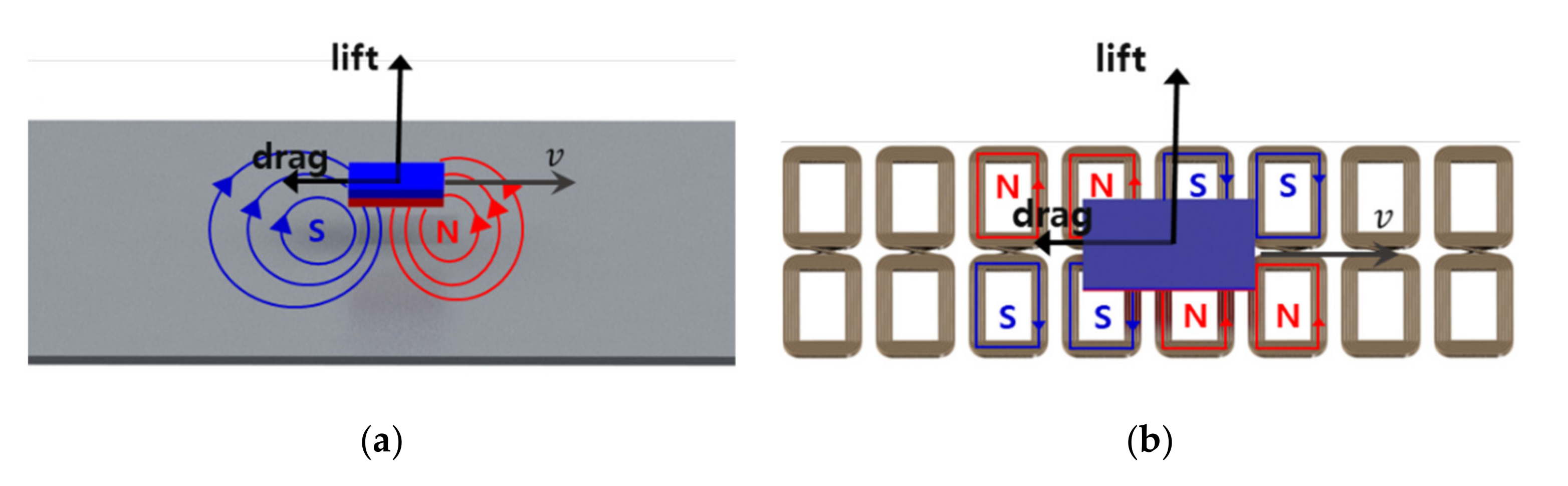
2. Basic Principles of Null-Flux EDS for the Hyperloop

In a Hyperloop system, the EDS uses the repulsive force between the onboard magnets and the induced current that occurs when the magnets pass over the electromagnetic track, which consists of conductors. Figure 1 shows two different track types, where a continuous sheet conductor with a certain thickness and electrically connected multi-turn coils are arranged. It also shows that the induced current caused by the physical phenomena that interfere with the magnet movement produces both drag and lift forces. Generally, continuous sheet tracks induce more current than discrete coil tracks, so they are better for onboard permanent magnets. However, discreet coil tracks use a null-flux connection that connects the terminals of two coils in a figure-eight shape, where the current is induced by the difference in the magnetic flux of the two connected coils. Therefore, the discrete null-flux track is more suitable for vehicles with SCMs that form a strong magnetic field.

Any magnetic levitation device for the Hyperloop should be suitable for lightweight vehicle design and dynamic safety at subsonic speeds. With the use of the null-flux EDS with onboard SCMs, a large physical air gap of up to 100 mm can be achieved, and subsonic driving stability without levitation control can be obtained. In addition, the detachable cryocooler technology makes the lightweight vehicle design suitable for rapidly transporting small groups of people. Therefore, the null-flux EDS technology is considered as an appropriate technology for Hyperloop systems.

Figure 2 shows a concept of the Hyperloop in which SCM mounted bogies move along an electromagnetic guideway attached to a side wall inside a sub-vacuum tube. The electromagnetic guideway, which consists of a linear synchronous motor (LSM) and a null-flux EDS track, accelerates the capsule train, which is mounted on bogies up to sub-vacuum speeds while it is magnetically levitated and guided. When the propelled SCM by the LSM moves in the +x-direction, the EDS track generates a vertical lift, and the horizontal guidance forces the SCM to move in the direction that restores it to the center of the EDS track, generating a drag force in the –x-direction of the SCMs.

As shown in Figure 3, the null-flux EDS track (or device) consists of a continuous arrangement of a null-flux levitation coil consisting of four levitation coils, and those coils, which are located on the same x position, are null-flux connected, as shown on the blue line. However, all the levitation coils are electrically insulated along the moving direction. As the null-flux coils are mostly configured in similar ways, the main design of the null-flux EDS device is to find a better levitation coil shape by the iterative process of analyzing the force response to the SCMs mounted on a moving bogie.

The sequential computation of the induced EMF and current and the force of the SCM are required for the performance analysis of the levitation coil. When the SCM moves at a velocity $\mathit{v}$ (the levitation coils move with a velocity ${\mathit{v}}_{\left(lev\right)}=-v$), the time-varying spatial MFD of the SCM induces EMF ${\epsilon }_i$ in the $i$-th levitation coil according to Faraday’s law. When the MFD ${\mathit{B}}_{\left(SCM\right)}$ of the SCM is calculated by numerical analysis or experimental measurement, the EMF in the $i$-th coil is expressed by Equation (1), where $\mathit{v}={\left[v_x, v_y, v_z\right]}^T$ is the velocity of the SCM, and ${\mathit{b}}_i={\left[b_{i\left(x\right)}, b_{i\left(y\right)}, b_{i\left(z\right)}\right]}^T$ denotes the coefficient vector of the induced EMF for the unit velocity vectors along the x, y, or z directions.

$${\epsilon }_i={\mathit{b}}_i^T\mathit{v}$$

(1)

With the change of the spatial ${\mathit{B}}_{\left(SCM\right)}$, ${\mathit{b}}_i$ can be represented as in Equation (2) using the mutual inductance $M_i={\mathsf{\Phi }}_i/I_{\left(SCM\right)}$ [16,18], where ${\mathsf{\Phi }}_i$ is the magnetic flux of the SCM in the $i$-th levitation coil. When the levitation coil moves at a velocity of $-\mathit{v}$, ${\mathit{b}}_i$ can be calculated as a line integral along the winding of the coil [26], as shown in Equation (3), where ${\mathit{e}}_{\left(d\right)}$ denotes the unit directional vector for the directions $d=x,y, \mathrm{or} z$. Although ${\mathit{b}}_i$ in Equation (2) is easy to understand, as it is explicitly related to a gradient of the SCM magnetic flux inside the coil, its computational cost is relatively high due to the surface integral of the MFD. Equation (3), however, seems to be a relatively complex formula, but the computation cost is relatively low as it requires a line integral of the MDF. In addition, if ${\mathit{B}}_{\left(SCM\right)}$ is pre-calculated, ${\mathit{b}}_i$ can be easily determined by the sum of the magnetic field values on the coil winding.

$$b_{i\left(d\right)}=-I_{\left(SCM\right)}\frac{\partial }{\partial d}{M}_i$$

(2)

$$b_{i\left(d\right)}=-{{\displaystyle \int }}_{C_i}{\mathit{e}}_{\left(d\right)}\times {\mathit{B}}_{\left(SCM\right)}•d\mathit{l}$$

(3)

For the induced EMF ${\epsilon }_i$, the induced current $I_i$ can be calculated by solving the following RL circuit equation flowing on the $i$-th coil of the inductance $L_i$ and resistance $R_i$.

$$\frac{d}{dt}{L}_i{I}_i+R_i{I}_i={\epsilon }_i$$

(4)

Although the force ${\mathit{f}}_i$ on the SCM can be calculated using the Lorentz force equation, further MFD analysis is required for the $i$-th coil with the induced current flowing. Instead, without any additional MFD analysis, the force can be simply calculated using Equation (5) by using the energy balance for the coil [18]:

$${\mathit{f}}_{i\left(lev\right)}^T\mathit{v}=I_i{\mathit{b}}_i^T\mathit{v}$$

(5)

where ${\mathit{f}}_{i\left(lev\right)}$ denotes the force on the coil, and the left and right sides represent the mechanical and electrical powers, respectively. Comparing both sides of Equation (5) results in ${\mathit{f}}_{i\left(lev\right)}$ in Equation (6), and ${\mathit{f}}_i$ in Equation (7) can be obtained by applying the force reaction ${\mathit{f}}_i=-{\mathit{f}}_{i\left(lev\right)}$.

$${\mathit{f}}_{i\left(lev\right)}=I_i{\mathit{b}}_i$$

(6)

$${\mathit{f}}_i=-I_i{\mathit{b}}_i.$$

(7)

As described so far, the force computation becomes simple when ${\mathit{b}}_i$ is determined. However, in order to improve the efficiency of the design model, the analysis concerning Equations (1)–(4) needs to be further simplified, and the simplified model would significantly improve the computation speed during the design of the null-flux EDS device.

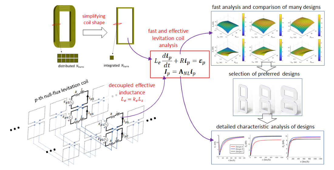
3. Design Model of the Null-Flux EDS Coils

3.1. Assumptions for Simplifying the Design Analysis

For the design of a null-flux EDS device, multi-turn and multi-layer coils are generally considered; however, the design is usually limited, as it needs to consider in-depth features when analyzing many coil designs. First, the cross-section of the levitation coil is simplified from the distributed N turns to the integrated N turns, as shown in Figure 4a, and then the coil shape is also simplified into a 2D rectangular shape based on the dynamic circuit theory. Such simplification can be applied to a null-flux EDS track when the SCM wires and levitation coils are sufficiently separated compared with the cross-section of the coil. Further, the magnetic coupling effects between the adjacent levitation coils are simplified by the constant multiplier of self-inductance. Then, the induced current and electromagnetic force can be written in closed-form solutions by the decoupled RL equations of the coils. As the coils are placed side by side, the coupling effects are expected to be lower in comparison with the coils that closely face each other, and the self-inductance $L_s$ can be dominant. In addition, the SCM that consists of pairs of N and S poles forms the periodic MFD along the moving direction, and thus the induced EMFs on the coils by the moving SCM is also periodic. In this case, the performance of many coil designs can be efficiently analyzed and relatively compared using the self-inductance without the coupling effect, and accurate results can be obtained by applying the effective inductance $L_e$ of Equation (8) multiplied by the appropriate coupling effect $k_e$ to the decoupled RL equations.

$$L_e=k_e{L}_s$$

(8)

The simplified rectangular coils are continuously placed in two layers in planes L and R, as shown in Figure 4b, and then the coil design is to find the simplified rectangular coil shape that shows the best performance. Further, the analysis model to be described in the following uses only SCM magnetic field in the plane L and R in which the levitation coils are placed, enabling faster computation. The induced EMF and current, and null-flux force models will be subsequently described for a null-flux EDS device.

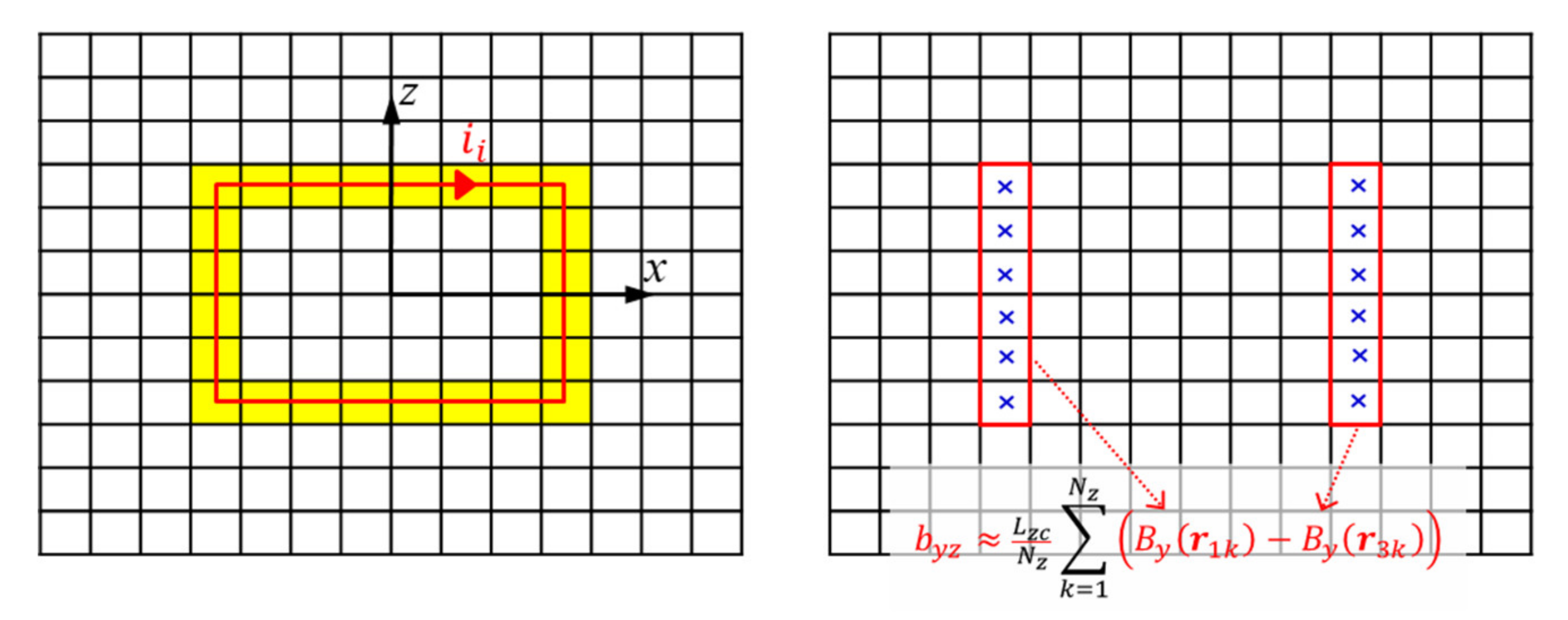
3.2. Induced EMF Model for the Levitation Coil

A line integral along the coil winding is usually required for the induced EMF computation. However, now, with the simplified rectangular shape of the levitation coil, the computation has become very easy. As shown in Figure 5, the rectangular closed curve C is sequentially connected by four sides in the +y axis direction: C1, C2, C3, and C4. When its vertical and horizontal lengths are $L_{zc}$ and $L_{xc}$, respectively, the positional vectors ${\mathit{r}}_1$,${\mathit{r}}_2$, ${\mathit{r}}_3$, and ${\mathit{r}}_4$ for the C1–C4 lines can be represented using the variables $\overline{x}=x/L_{xc}$ and $\overline{z}=z/L_{zc}$, which are normalized by the length of each side.

$${\mathit{r}}_1=-\frac{L_{xc}}{2}{\mathit{e}}_x+L_{zc}\overline{z}{\mathit{e}}_z$$

(9)

$${\mathit{r}}_2=L_{xc}\overline{x}{\mathit{e}}_x+\frac{L_{zc}}{2}{\mathit{e}}_z$$

(10)

$${\mathit{r}}_3=\frac{L_{xc}}{2}{\mathit{e}}_x-L_{zc}\overline{z}{\mathit{e}}_z$$

(11)

$${\mathit{r}}_4=-L_{xc}\overline{x}{\mathit{e}}_x-\frac{L_{zc}}{2}{\mathit{e}}_z$$

(12)

where $-1/2\le \overline{x}\le \frac{1}{2} \mathrm{and} -1/2\le \overline{z}\le 1/2$.

When the SCM moves at a velocity $\mathit{v}$, the induced EMF in the levitation coil is expressed as in Equations (1) and (3), and by substituting the Equations (9)–(12) into Equation (3), the induced EMF coefficient vector $\mathit{b}$ can be expressed as

$$\mathit{b}={\left[\begin{array}{ccc}{b}_x& b_y& b_z\end{array}\right]}^T= {\left[\begin{array}{ccc}-b_{yz}& b_{xz}-b_{zx}& b_{yx}\end{array}\right]}^T$$

(13)

$$b_{iz}=N_{turn}{L}_{zc}{{\displaystyle \int }}_{-1/2}^{1/2}\left(B_i\left({\mathit{r}}_1\right)-B_i\left({\mathit{r}}_3\right)\right)d\overline{z} \mathrm{for} i=x, y$$

(14)

$$b_{jx}=N_{turn}{L}_{xc}{{\displaystyle \int }}_{-1/2}^{1/2}\left(B_j\left({\mathit{r}}_2\right)-B_j\left({\mathit{r}}_4\right)\right)d\overline{x} \mathrm{for} j=y, z,$$

(15)

where $=$ ${\left[v_x v_y v_z\right]}^T$, and $\mathit{B}={\left[B_x B_y B_z\right]}^T$ is the MFD of the SCM.

Since the MFD of the SCM has a sinusoidal wave form, for faster calculations, the Riemann sum can be considered as an approximation of the integral of Equations (14) and (15). When the horizontal and vertical lengths $L_{xc}$ and $L_{zc}$ are divided into sufficiently large $N_x$ and $N_z$ subintervals, the position vectors ${\mathit{r}}_{1k}$,${\mathit{r}}_{2k}$, ${\mathit{r}}_{3k}$, and ${\mathit{r}}_{4k}$ of the four sides can be expressed for the k-th subinterval using the normalized evaluating medium points of the subintervals ${\overline{x}}_k$ or ${\overline{z}}_k$.

$${\mathit{r}}_{1k}=-\frac{L_{xc}}{2}{\mathit{e}}_x+L_{zc}{\overline{z}}_k{\mathit{e}}_z$$

(16)

$${\mathit{r}}_{2k}=L_{xc}{\overline{x}}_k{\mathit{e}}_x+\frac{L_{zc}}{2}{\mathit{e}}_z$$

(17)

$${\mathit{r}}_{3k}=\frac{L_{xc}}{2}{\mathit{e}}_x-L_{zc}{\overline{z}}_k{\mathit{e}}_z$$

(18)

$${\mathit{r}}_{4k}=-L_{xc}{\overline{x}}_k{\mathit{e}}_x-\frac{L_{zc}}{2}{\mathit{e}}_z$$

(19)

$${\overline{x}}_k=-\frac{1}{2}+\frac{\left(2k-1\right)}{2N_x}$$

(20)

$${\overline{z}}_k=-\frac{1}{2}+\frac{\left(2k-1\right)}{2N_z}$$

(21)

Then, by using Equations (16)–(21), Equations (14) and (15) can be approximated by the sum of the MFD of the SCM:

$$b_{iz}\approx \frac{L_{zc}}{N_z}{{\displaystyle \sum }}_{k=1}^{N_z}\left(B_i\left({\mathit{r}}_{1k}\right)-B_i\left({\mathit{r}}_{3k}\right)\right) \mathrm{for} i=x, y$$

(22)

$$b_{jx}\approx \frac{L_{xc}}{N_x}{{\displaystyle \sum }}_{k=1}^{N_x}\left(B_j\left({\mathit{r}}_{2k}\right)-B_j\left({\mathit{r}}_{4k}\right)\right) \mathrm{for} j=y, z.$$

(23)

When the MFD changes caused by levitation coils are effectively shielded by cryostat and radiation shield of the SCM, the specific MFD of the SCM operated by DC current can be used repeatedly after pre-calculation. To characterize the MFD of the SCM required for the calculation of $\mathit{b}$, general numerical methods, such as FEM and boundary element method (BEM), experimentally measured data, or a distributed multilevel current (DMC) model that utilizes equivalent magnetizing point currents to describe the MFD of electromagnetic components [27], can be used. For example, Figure 6 shows the MFD pattern of the SCM with a magnetomotive force (MMF) of 300 kAt that consists of a pair of N and S poles computed by the DMC model for the fast computation of the MFD, and $\mathit{b}$ can be easily obtained by applying the MFD to Equations (22) and (23). If the characteristics of $\mathit{b}$ for the SCM, which consists of N and S pole pairs, are further analyzed, for the z-axis, $B_x$ is symmetric and $B_y$ and $B_z$ are anti-symmetric. However, for the x-axis, $B_x$ and $B_y$ are symmetric and $B_z$ is anti-symmetric. Also, according to Equations (22) and (23), $b_{x }$=$-b_{yz}$ is an even function, and $b_y=b_{xz}-b_{zx}$ and $b_z=b_{yx}$ are odd functions for the x-axis.

Once b is determined, the induced EMF $\epsilon$ can be determined by Equation (1). For example, if the SCM moves along the +x-direction, then $v=v_x{e}_x$ and $\epsilon =b_x{v}_x=-b_{yz}{v}_x$ for the levitation coil. Figure 7 shows how the $b_{yz}$ for the induced EMF can be easily calculated for the simplified levitation coil in the yellow rectangular shape. From Equation (22), $b_{yz}$ only requires the surface normal magnetic field $B_y$, which is marked by a blue x on the left and right sides. Also, computing $b_{yz}$ is the simple summation and difference operation of $B_y$ for each of the left and right vertical sides denoted by the red rectangles. The other $b_{iz}$ and $b_{jx}$ can also be easily calculated in a similar way.

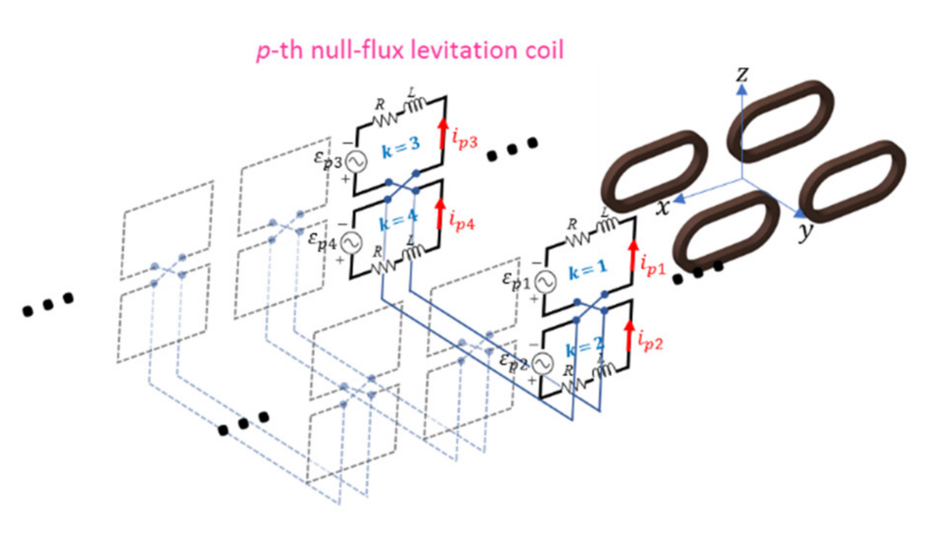
3.3. RL Circuit Analysis for the Induced Current

The induced current on the levitation coil can be obtained by solving the RL circuit equation, which consists of the induced EMF ε, the resistance R, and the inductance L on each levitation coil. However, the RL circuit analysis for the arbitrary induced voltage input increases the overall computation time by using a numerical ODE solver. Therefore, if the induced EMF ε that is generated in the levitation coil by the SCM is expanded into the Fourier series, the induced current at each frequency can be easily calculated, and the resulting induced current can be obtained from the summation.

When the center of the SCM in the moving direction is fixed at the origin, the relative position of the levitation coil $x_c$ that is moving at $\mathit{v}=-v_x{\mathit{e}}_x$ is

$$x_c= x_m-v_{x}t$$

(24)

where $x_m$ is the maximum displacement of the levitation coil from the center of the SCM, and it becomes $- x_m\le x_c\le$ $x_m$. Actually, $x_m$ denotes half the maximum track length of the levitation coil to be considered, so it requires to be several times larger than ${\tau }_{SCM}\times N_{SCM}$, where ${\tau }_{SCM}$ and $N_{SCM}$ represent the pole pitch and the number of poles of the SCM, respectively. In addition, for the Fourier series expansion in the entire defined range of $x_c$, $x_m$ would be the integer n multiple of the ${\tau }_{SCM}$, where the angular velocity ${\omega }_n$ can be defined as

$${\omega }_n=\frac{2n\pi }{x_{max}-x_{min}}=-\frac{n\pi }{x_m}.$$

(25)

Since $b_x=-b_{yz}$, which is defined by $B_y$ difference of the left and right sides, as shown in Figure 7, is an even function, $b_x$ can be represented by the Fourier cosine series, and the odd functions $b_y$ and $b_z$ can be expanded by the Fourier sine series.

$$b_x={\displaystyle \sum }_n{A}_n\cos ({\omega }_n{x}_c)$$

(26)

$$b_y={\displaystyle \sum }_n{B}_n\sin \left({\omega }_n{x}_c\right)$$

(27)

$$b_z={\displaystyle \sum }_n{C}_n\sin \left({\omega }_n{x}_c\right),$$

(28)

where $A_n$, $B_n$, and $C_n$ are the Fourier coefficients for $b_x$, $b_y$, and $b_z$, respectively. Also, the induced current $i\left(x\right)$ can be expressed as the sum of the induced current response $i_n\left(x\right)$ at the n-th harmonic frequency:

$$i\left(x_c\right)={\displaystyle \sum }_n{i}_n\left(x_c\right).$$

(29)

When Equation (24) is applied to Equation (4) and combined with Equations (26) and (29), the RL circuit equation of the n-th harmonic frequency for the relative position $x_c$ is expressed as

$$-L{v}_x\frac{d{i}_n}{d{x}_c}+R{i}_n=v_x{A}_n\cos ({\omega }_n{x}_c).$$

(30)

After excluding the transient response by the initial conditions, a solution of $i_n\left(x\right)$ becomes a combination of cosine and sine functions.

$$i_n\left(x_c\right)=\frac{A_n{v}_x}{{\omega }_n{}^2{(L{v}_x)}^2+R^2}\left(-{\omega }_{n}L{v}_x\sin ({\omega }_n{x}_c\right)+R\cos ({\omega }_n{x}_c)).$$

(31)

Thus, the reaction force $\mathit{f}\left(x_c\right)$ to the SCM is obtained by either applying $i\left(x_c\right)$ in Equation (29) to Equation (7), or by summing of the response force ${\mathit{f}}_n\left(x_c\right)$ at n-th harmonic frequency, which is calculated by applying Equations (31) and (26)–(28) to Equation (7):

$${\mathit{f}}_n\left(x_c\right)=-i_n\left(x_c\right){\left[\begin{array}{ccc}{A}_n\cos ({\omega }_n{x}_c)& B_n\sin \left({\omega }_n{x}_c\right)& C_n\sin \left({\omega }_n{x}_c\right)\end{array}\right]}^T.$$

(32)

To investigating the characteristics of the levitation coil, the average force ${\mathit{f}}_{n\left(avg\right)}\left(x_c\right)$ can be calculated by averaging Equation (32) for the periodic intervals:

$${\mathit{f}}_{n\left(avg\right)}\left(x_c\right)=-\frac{A_n{v}_x}{2({\omega }_n{}^2\left(L{v}_x{)}^2+R^2\right)}{\left[\begin{array}{ccc}{A}_{n}R& B_n{\omega }_{n}L{v}_x& C_n{\omega }_{n}L{v}_x\end{array}\right]}^T$$

(33)

where the negative sign appears as a reverse movement of the levitation coil from $x_m$ to $- x_m$. The lift and guidance forces have similar characteristics, and the overall characteristics mainly depend on the Fourier coefficients defined according to the MFD and the coil design. Also, the inductance and speed effects appear to be relatively large. The drag force acting in the –x-direction always occurs in a direction that prevents the SCM from moving, and the resistance effect seems to be dominant. If the speed continues to increase, as the effect of the resistance gradually decreases, the inductance effect continues to increase, and at extremely high speeds, only the inductance effect would remain:

$$\underset{v\to \infty }{\lim }{\mathit{f}}_{n\left(avg\right)}\left(x_c\right)=-\frac{A_n}{2\left(w_{n}L\right)}{\left[\begin{array}{ccc}0& B_n& C_n\end{array}\right]}^T$$

(34)

This implies that the inductance has a dominant effect on the performance of subsonic levitation devices.

3.4. Force Formulation of the Null-Flux EDS Device and Track

Even though the induced EMF and current are calculated for each coil, the actual voltage and current acting on the coils change with the null-flux connection. The null-flux EDS device consists of a number of null-flux levitation coils, as shown in Figure 8, where the p-th null-flux levitation coil, which consists of four coils, gives the coils a number of $k=1,\dots ,4$ from the top left to the bottom right.

When all the coils have identical R and L values, the effective voltage ${\mathit{V}}_p$ in the null-flux connection can be determined by the null-flux relation matrix $A_{NL}$ and the induced EMF vector ${\mathit{\epsilon }}_p$:

$${\mathit{V}}_p={\mathit{A}}_{NL} {\mathit{\epsilon }}_p, {\mathit{A}}_{NL}=\frac{1}{4}\left[\begin{array}{c}\begin{array}{cc} 3& -1\\ -1& 3\end{array} \begin{array}{cc}-1& -1\\ -1& -1\end{array}\\ \begin{array}{cc}-1& -1\\ -1& -1\end{array}\begin{array}{cc} 3& -1\\ -1& 3\end{array}\end{array}\right],$$

(35)

where ${\mathit{V}}_p={\left[\begin{array}{cc}{V}_{p1}& V_{p2}\end{array} \begin{array}{cc}{V}_{p3}& V_{p4}\end{array}\right]}^T$, ${\mathit{\epsilon }}_p={\left[\begin{array}{cc}{\epsilon }_{p1}& {\epsilon }_{p2}\end{array} \begin{array}{cc}{\epsilon }_{p3}& {\epsilon }_{p4}\end{array}\right]}^T$, and the subscript pk represents the k-th levitation coil, which consists of p-th null-flux levitation coils. For the current ${\mathit{i}}_p={\left[i_{p1} i_{p2} i_{p3} i_{p4}\right]}^T$ induced by ${\mathit{\epsilon }}_p$, the resultant current ${\mathit{I}}_p={\left[I_{p1} I_{p2} I_{p3} I_{p4}\right]}^T$ in the null-flux coil can be determined using $A_{NL}$:

$${\mathit{I}}_p={\mathit{A}}_{NL}{\mathit{i}}_p.$$

(36)

In order to evaluate the performance of the null-flux EDS device, it is also necessary to calculate the force change that occurs during the SCM driving. As shown in Figure 9, when the SCM, which is located on the $P_0$ with the vertical ∆z and horizontal ∆y displacements, moves along the x-direction, the force from the p-th null-flux levitation coil to the SCM is the sum of the k-th coil forces ${\mathit{f}}_{pk}$ computed by Equations (32) and (7). When the x position of the p-th null-flux levitation coil is $x_{p0}$, the relative position for the moving SCM becomes $x_p$=$x_{p0}-\Delta x$, and the resultant force $\mathit{f}\left(\Delta x\right)$ acting on the SCM located in $\Delta x$ is expressed as the sum of the forces from a total of P null-flux levitation coils, each consisting of four levitation coils:

$$\mathit{f}\left(\Delta x\right)={\displaystyle {\displaystyle \sum }_{p=1}^P}{\displaystyle {\displaystyle \sum }_{k=1}^4}{\mathit{f}}_{pk}\left(x_{p0}-\Delta x\right).$$

(37)

4. Examples and Validation

As an illustrative application of the SLC model, a null-flux EDS device was designed for a small-scale testbed. The design parameters of the SCM and EDS devices were first listed, the analysis results of the designs using the SLC model were summarized, and the best designs were selected based on the performance criteria. Subsequently, for the validation of the SLC model, the variation of the average lift force was compared with the results of the FEM analysis by changing the design parameters. Also, for the selected designs, the SLC model was validated by comparing the force changes with the FEM analysis results when the bogie with the SCM was moving. During the validation step, the 3D FEM results, which were analyzed in the Simcenter MagNet, were used, and the half-symmetric and full models were applied to the $P_z$ and $P_y$ positions, respectively. Finally, the performance change of the designed EDS devices was calculated when the driving position or speed of the SCM changed, and then the difference in the performance and characteristics among the EDS devices was discussed.

4.1. Design Parameters for the Illustrative Application

As shown in Figure 10, two modules of the SCMs are placed on both the left and right sides of a bogie, where each one of them consists of two poles. Here, we aimed at testing the performance of the propulsion and levitation devices for Hyperloop systems at a relatively low cost. The SCM should be developed by lowering the cost with a relatively small pole pitch ${\tau }_{SCM}$ and MMF, and its main design specifications are listed on the right side of Figure 10. The total weight of the bogie, including the two SCMs, is targeted at around 1.35 tons, but the EDS devices were designed to have more than enough lift and guidance forces without an upper limit.

The multiple design parameters affect the performance of the null-flux EDS device, as shown in Figure 11, where the levitation coils are arranged by the pole pitch ${\tau }_c$ and gap $d_x$ in the x-direction, and the vertical and horizontal coil lengths are $L_{zc}$ and $L_{xc}$. Also, the cross-sectional wire area $A_w$ is the product of the wire width $c_w$ and thickness $c_t$, and the number of turns $N_{turn}$ is multiplied by the number of turns $N_w$ in the xz plane and $N_t$ in the y-direction. For an effective illustration of the SLC model, the ${\tau }_c$, $N_{turn}$, and $L_{zc}$, which can significantly affect the performance, were selected as the design variables of the levitation coil, and all the other design parameters were specified. The derived parameters should be physically constrained to have a feasible shape. Thus, the stacked coil thickness $L_{cw}$ can become the product of $c_w$ and $N_w$, $L_{xc}$ can be determined in relation to $d_x$ and $L_{cw}$, and the vertical core position $z_c$ can become half the sum of $L_{cw}$ and $L_{zc}$.

The levitation and guidance performance at the maximum vertical displacement point $P_z=(0, -\Delta z_{max})$ and maximum horizontal displacement $P_y=(-\Delta y_{max}, -\Delta z_{max}/2)$ were compared when the horizontal and vertical displacements reached their maximum values $\Delta y_{max}$ and $\Delta z_{max}$. The performance was mainly evaluated at a subsonic driving velocity $v_h$, and it also considered the take-off velocity $v_l$ for the design. Since the physical air gap at the center position is $g_{air}$, and the thickness of the levitation coil is $L_t$, the simplified coil was designed at plane L or R, which are located in the $g_{air}$+$L_t/2$ from the SCM surface. The performance of the EDS device could be evaluated at various positions and speeds, and different weight factors could be applied to the lift and guidance forces. In this example, the primary design criterion is to maximize the lift force at $P_z$ for the driving velocity $v_h$, and the other performance values, such as the guidance and drag forces or the different speeds and positions, were calculated and compared against the selected designs. All the design parameters and variables related to the EDS devices are summarized in

Table 1. Design parameters of the null-flux EDS device for the small-scale Hyperloop testbed.

Parameter	Value	Unit
Number of turns, $N_{turn}=N_w\times N_t$	$N_t=2$ $N_w=4,5,\dots , 14, 15$	turns
Pole pitch,${\tau }_c$	(1/6, 1/5, 1/4, 1/3, 2/5, 1/2, 3/5, 2/3, 3/4, 4/5, 5/6)$\times {\tau }_{SCM}$	$\mathrm{m}$
Vertical coil height, $L_{zc}$	$0.2, 0.22, \dots , 0.38, 0.4$	$\mathrm{m}$
Wire cross sectional area, $A_w=c_w\times c_t$	$0.01\times 0.01$	${\mathrm{m}}^2$
Horizontal gap between coils, $d_x$	$0.03$	$\mathrm{m}$
Horizontal coil width, $L_{xc}$	${\tau }_c-d_x-c_w{N}_w$	$\mathrm{m}$
Vertical core position, $z_c$	$\left(L_{zc}+c_w{N}_w\right)/2$
Aluminum wire conductivity, ${\sigma }_{alu}$	$3.77\times {10}^7$	$\mathrm{S}/\mathrm{m}$
Air gap, $g_{air}$	$0.05$	$\mathrm{m}$
Thickness of the levitation coil, $L_t$	$0.03$	$\mathrm{m}$
Half of the track length, $x_m$	$13\times {\tau }_{SCM}$	$\mathrm{m}$
Number of the levitation devices, $P$	$12$	-
Subsonic driving velocity, $v_h$	$277.78 \left(1000\right)$	m/s ($\mathrm{km}/\mathrm{h}$)
Take off velocity, $v_l$	$41.67 \left(150\right)$	m/s ($\mathrm{km}/\mathrm{h})$
Maximum vertical displacement, $\Delta z_{max}$	$0.10$	$\mathrm{m}$
Maximum horizontal displacement, $\Delta y_{max}$	$0.05$	$\mathrm{m}$

, and the performances of a total of 1452 designs were analyzed and compared at different speeds and locations.

4.2. Design Model for the Illustrative Application

4.2.1. Resistance and Inductance Approximation

The SLC model requires a coil resistance and inductance according to the changes in the design parameters, and the approximated equations can be considered for the fast analysis of many design cases. As shown by the red line in Figure 11, the coil resistance $R$ of the aluminum wire with the conductivity ${\sigma }_{alu}$ can be simply approximated using the simplified rectangular coil:

$$R\left(\mathsf{\Omega }\right)=\frac{2N_{turn}\left(L_{xc}+L_{zc}\right)}{{\sigma }_{alu}{A}_w}.$$

(38)

Although the inductance is important for evaluating the coil performance, accurate numerical analyses lead to high computational loads. Therefore, as the SLC model finds a better-performing design among the different design cases, the self-inductance approximation, which can be quickly calculated with a certain level of accuracy, can be used with Equation (8), where $k_e=1$. In the case of the self-inductance of the square core coils, various approximations can be applied depending on the winding patterns. Since the effect of $N_w ,$ which is the number of spiral turns on the design plane, is important, this design example uses the following inductance approximation of the flat spirals with the polygonal turns [28,29]:

$$L_a \left(\mathsf{\mu }\mathrm{H}\right)=0.8s{\left(N_{turn}\right)}^2\left[\ln \frac{L_{xc}+ L_{zc}}{2N_w{c}_w}+0.72599+0.1776\frac{2N_w{c}_w}{L_{xc}+ L_{zc}}+0.125{\left(\frac{2N_w{c}_w}{L_{xc}+ L_{zc}}\right)}^2\right].$$

(39)

For the EDS device with ${\tau }_c=\left(2/3\right){\tau }_{SCM}$, the resistance and inductance are approximated using Equations (38) and (39). The calculated values for changing $L_{zc}$ and $N_{turn}$ are depicted in Figure 12, where both values increase with the increase in $L_{zc}$ and $N_{turn}$, as the inductance nonlinearly and rapidly increases unlike linearly increasing resistances.

4.2.2. Fourier Series Analysis of the Induced EMF

For the accurate computation of the induced current, the Fourier series expansion of $b_x$ needs to be included in the calculation up to a frequency that can be accurately represented in all ranges where the levitation coils are placed, such as $b_x$ for the SCM position $P_y$. Also, the evaluating coil number $k=3$ was selected, as it is involved in large changes of the magnetic field with the end effect of the SCM. $b_x$ in Equation (26) was expanded as a Fourier series for various maximum $n$, $n_{max}$, as shown in Figure 13a, where the scope of ${\tau }_c/ {\tau }_{SCM}$ was enlarged, including the magnification plots near the peak value, to check for any errors. It shows that the accuracy of the Fourier series improves with the increase in $n_{max}$. With respect to the original $b_x$ that is corresponding to $n_{max}=\infty$ case, the RMSE (root mean square error) of at each $n_{max}$ was calculated to evaluate the accuracy of the Fourier series:

$$RMSE={\left[{\displaystyle \sum }_{i=1}^N{\left(b_{n_{max}}\left(x_i\right)-b_{inf}\left(x_i\right)\right)}^2/N\right]}^{1/2}$$

(40)

where evaluating coil positions $N=4001$, $b_n$ and $b_{inf}$ denote the $b_x$ for the $n_{max}=n$ and $\infty$, respectively. Figure 13b also compares the Fourier coefficients and RMSE values with the changes in the $n_{max}$ values. Although the $n_{max}$ increased, the Fourier coefficient value was similar, and the values close to the maximum frequency appeared to be out of trend. Based on the compared $b_x$ and evaluated RMSE, it appears that the $n_{max}$ seemed appropriate at least 100. Since the induced current is the sum of the closed-form Equation (31) by calculating the n times, the increase in the computational load with the increase in the $n_{max}$ was small, so the computational accuracy increased by including up to $120-{\mathrm{th}}^{}$ harmonics of the $b_x$ in this example.

4.3. Design Results for the Illustrative Application

To design EDS devices suitable for the SCM, as shown in Figure 10, the performance changes for the design variables (${\tau }_c$, $N_{turn}$, and $L_{zc}$) were analyzed and discussed using the SLC model. The performance was compared at the $P_z$ and $P_y$ positions not only for the lift and guidance forces but also for each of the force ripples $F_r$, which is defined as follows:

$$F_r\left(\%\right)=\left|\left(F_{max}-F_{min}\right)/2F_{avg}\right|\times 100$$

(41)

where $F_{max}$, $F_{min}$, and $F_{avg}$ are the maximum, minimum, and average forces in the $x, y, \mathrm{or} z$ directions, as shown by Equation (37).

First, to compare the changed shape and performance by the ${\tau }_c$, the designs for the pole pitches that produce the maximum lift force at $P_z$ and $v_h$ were selected and compared. Also, the design variables that maximize the lift force at each pole pitch are shown in Figure 14a, where $N_{turn}$ linearly increased with the increase in the pole pitch ratio ${\tau }_c/{\tau }_{SCM}$; however, $L_{zc}$ slightly decreased. For each design, the calculated vertical core position $z_c$ slightly increased as the pole pitch increased, which implies that the vertical distance between the coil cores remained at a certain value to increase the lift force when evaluated at $P_z$. The performances of the selected designs are compared in Figure 14b. It looks like the maximum lift force at $P_z$ continuously increased with the increase in the pole pitch ratio and then slightly decreased over $2/3$. The maximum guidance force of $P_y$ was similar in the pole pitch ratio of more than 1/3, with the highest in 1/2.

In view of the lift and guidance force ripples $F_{zr}$ and $F_{yr}$, the pole ratio of more than 2/3 seems to be difficult to use in practice due to the surge in the force ripple, and the guidance ripple is relatively high in the pole pitch ratios of 1/4 and 1/3.

The overall performances of the pole pitch ratios 2/5, 1/2, 3/5, and 2/3 seem to be good. However, considering that the three-phase LSMs, which are installed together, generally have a 1/3 or 2/3 pole pitch ratio, the 1/2 and 2/3 pole pitch ratios that have relatively small common multiples for the pole pitch ratio of the LSM were selected for the detailed analysis. In addition, it is also necessary to include the 1/3 pole pitch ratio in the detailed analysis as a contrast design, since it is applied to the superconducting Maglev series L0 [7].

Next, the lift force $F_z$ at $P_z$ and the guidance force $F_y$ at $P_y$ were computed for the driving velocity $v_h$ in the selected pole pitch designs, and the force variations for the $N_{turn}$ and $L_{zc}$ are shown in Figure 15. If $L_{zc}$ increases or decreases from the design of the maximum lift force, $N_{turn}$ remains high, and it appears to be related to the high performance near a specific vertical core position. In general, it is desirable to find the desired design that can create an appropriately balanced lift and guidance forces. For the design with the small $L_{zc}$, the guidance force is increased, but its lift force is much lower. However, the design with the maximum lift force can lead to a reasonably good guidance force. Considering that securing a sufficient lift force is important in the small-scale testbed, three designs with the maximum lift force at each pole pitch were further analyzed and validated. 3D CAD models of the selected levitation coils are shown in Figure 16, and the design variables ${\tau }_c$, $N_{turn}$, and $L_{zc}$ are summarized in

Table 2. The three selected designs to be further analyzed and validated.

Design	${\mathit{\tau }}_{\mathit{c}}/{\mathit{\tau }}_{\mathit{S}\mathit{C}\mathit{M}}$	${\mathit{L}}_{\mathit{z}\mathit{c}}\left(\mathbf{m}\right)$	${\mathit{N}}_{\mathit{t}\mathit{u}\mathit{r}\mathit{n}}$	${\mathit{F}}_{\mathit{z}}\left(\mathbf{k}\mathbf{N}\right)$$\mathbf{at} {\mathit{P}}_{\mathit{z}}$	${\mathit{F}}_{\mathit{y}}\left(\mathbf{k}\mathbf{N}\right)$$\mathbf{at} {\mathit{P}}_{\mathit{y}}$
A	1$/3$	$0.29$	$12$	16.04	8.15
B	1$/2$	$0.28$	$18$	22.17	9.47
$\mathrm{C}$	$2/3$	$0.28$	$24$	24.39	8.84

, which shows that the maximum guidance force $F_y$ is more than a third of the maximum lift force $F_z$.

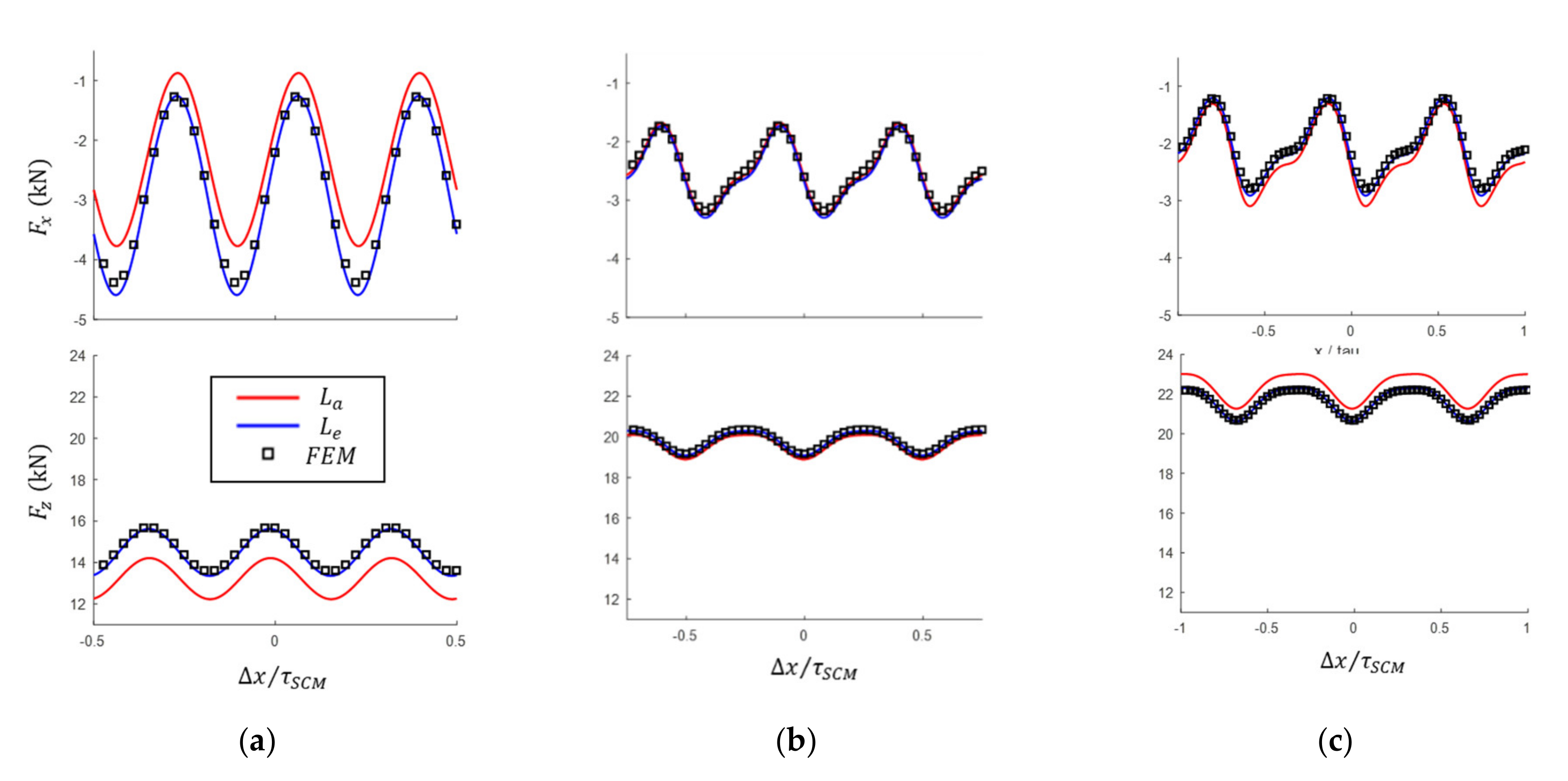
4.4. Design Model Validation with the FEM Results

To validate the SLC model, the lift force was analyzed by the FEM for the designs in which $N_{turn}$ or $L_{zc}$ were changed from Design C, and the results were compared with the computed results using the SLC model, as shown in Figure 17a,b, respectively. The SLC model uses the results of the approximated $L_a$ of Figure 12b and the numerical computed self-inductance $L_s$, where the coupling effects $k_e=1$ and $k_e=1.15$ are applied, respectively. The results from the FEM analysis generally showed a relatively small lift force than the SLC model; it was caused by the larger effective inductance due to the mutual inductance. The changes in the lift force trends of $N_{turn}$ or $L_{zc}$ in the three analyses are very similar, and the best design results are also very similar: $N_{turn}$ of $22–24$ turns and $L_{zc}$ of $0.26~0.28 \mathrm{m}$. Since matching the analyzed trends is most important for selecting relatively better designs, the SLC model was validated through the FEM results.

When the accuracy of the calculated force is also important in the analysis of the design characteristics, an easy way to obtain accurate results for various conditions is by applying the obtained $k_e$ values from the reference results using the analysis or the experiment of the SLC model. Since the lift force in the high-speed section is inversely proportional to the inductance, as per Equation (34), for the averaged reference force $f_e$ of the effective inductance $L_e$ and the SLC force $f_s$ of the self-inductance $L_s$, the coupling effect $k_e$ can be determined as

$$k_e=\frac{f_s}{f_e}.$$

(42)

Thus, $L_e$ can be determined by Equation (8). For the three designs in Table 2, the determined $L_e$ and the respective $k_e$ and ${k_e}^{\prime }$ for $L_a$ and $L_s$ are summarized in

Table 3. Calculation of the coupling effect and effective inductance values for the three selected designs.

Design	${\mathit{\tau }}_{\mathit{c}}/{\mathit{\tau }}_{\mathit{S}\mathit{C}\mathit{M}}$	${\mathit{L}}_{\mathit{a}}\left(\mathsf{\mu }\mathbf{H}\right)$	${\mathit{L}}_{\mathit{s}}\left(\mathsf{\mu }\mathbf{H}\right)$	${\mathit{L}}_{\mathit{e}}\left(\mathsf{\mu }\mathbf{H}\right)$	${{\mathit{k}}_{\mathit{e}}}^{\prime }$$\mathbf{for} {\mathit{L}}_{\mathit{a}}$	${\mathit{k}}_{\mathit{e}}$$\mathbf{for} {\mathit{L}}_{\mathit{s}}$
A	1$/3$	$58.06$	$48.60$	$50.52$	0.8701	1.0395
B	1$/2$	141.99	$125.68$	$140.21$	0.9875	1.1156
$\mathrm{C}$	$2/3$	$282.85$	$250.19$	$293.32$	1.0370	1.1724

. The $k_e$ values for $L_s$ are all greater than 1, so the effective inductances were increased due to the coupling effect of the mutual inductance. Also, as $k_e$ increases with the pole pitch, the effect of the mutual inductance increases with the increase in the pole pitch. The ${k_e}^{\prime }$ is less than $k_e$, and the two designs are less than 1, which was caused by the approximated $L_a$, which tends to overestimate the exact self-inductance. The trend of the change in $k_e$ for the change in $N_{turn}$ or $L_{zc}$ can also be analyzed by comparing the results shown in Figure 17a,b, respectively, where the coupling effect $k_e$ appears to increase with the increase in $N_{turn}$ or the decrease in $L_{zc}$, as $k_e$ can be determined by the force differences of the FEM and the $L_s$ applied SLC model.

The SLC model was validated by comparing the FEM results with $L_a$ or with the $L_e$ applied SLC model for the selected designs. Also, the performance and characteristics of each design were compared and analyzed. To compare the performance of the designs, the changes in the drag and lift forces in $v_h$ or $v_l$ at the $P_z$ were compared, as shown in Figure 18 and Figure 19, respectively, where the zero guidance force was not included in the comparison. Also, all the reaction force changes in $v_h$ at $P_y$ were compared in Figure 20. The pattern of the calculated force with $L_e$ matches the FEM results, but an offset due to the approximation error of $L_a$ can be observed. Meanwhile, in all cases, the results of the SLC model calculation with $L_e$ instead of $L_a$ greatly improved the accuracy. Especially, the drag and lift forces very closely agreed with the FEM results. In the $P_y$ position, where the SCM is closest to one side of the levitation coils, there is some difference in the guidance force result of Design A and B, which can be caused by the error in the $b_y$ calculation of Equation (13), in which the simplified coil shape of the SLC is calculated as the difference between two line integral quantities, $b_{xz}$ and $b_{zx}$.

To clearly compare the performance of each design with explicit numbers, the average forces and the calculated force ripples (%) by Equation (41) are summarized in

Table 4. Average forces and ripples for comparing the design performances.

Design	${\mathit{\tau }}_{\mathit{c}}/{\mathit{\tau }}_{\mathit{S}\mathit{C}\mathit{M}}$	${\mathit{P}}_{\mathit{z}}$$\mathbf{at} {\mathit{v}}_{\mathit{h}}$		${\mathit{P}}_{\mathit{z}}$$\mathbf{at} {\mathit{v}}_{\mathit{l}}$		${\mathit{P}}_{\mathit{y}}$$\mathbf{at} {\mathit{v}}_{\mathit{h}}$
		${\mathit{F}}_{\mathit{x}} {\left({\mathit{F}}_{\mathit{x}\mathit{r} }\right)}^1$	${\mathit{F}}_{\mathit{z}} \left({\mathit{F}}_{\mathit{z}\mathit{r} }\right)$	${\mathit{F}}_{\mathit{x}} \left({\mathit{F}}_{\mathit{x}\mathit{r} }\right)$	${\mathit{F}}_{\mathit{z}} \left({\mathit{F}}_{\mathit{z}\mathit{r} }\right)$	${\mathit{F}}_{\mathit{x}} \left({\mathit{F}}_{\mathit{x}\mathit{r} }\right)$	${\mathit{F}}_{\mathit{y}} \left({\mathit{F}}_{\mathit{y}\mathit{r} }\right)$	${\mathit{F}}_{\mathit{z}} \left({\mathit{F}}_{\mathit{z}\mathit{r} }\right)$
A	1$/3$	−0.55	18.39	−2.90	14.49	−0.27	9.34	19.70
		(293.98)	(6.33)	(57.40)	(7.83)	(641.11)	(24.52)	(7.79)
B	1$/2$	−0.44	22.46	−2.57	19.81	−0.20	9.59	23.78
		(243.50)	(3.29)	(30.45)	(3.08)	(375.21)	(9.36)	(7.81)
$\mathrm{C}$	$2/3$	−0.34	23.52	−2.08	21.66	−0.15	8.53	23.70
		(202.32)	(3.12)	(40.96)	(3.86)	(279.39)	(7.47)	(2.66)

¹ Units of the force and ripple are in kN and %, respectively.

. The drag ripple was found to be very high, as the acting direction continued to change, and its averaged value was very small compared with the other forces, as the larger the pole pitch of the design, the smaller the drag force. The lift force in the horizontal center position $P_z$ at $v_h$ was high in Designs B and C, but the lift force in Design A was small (78–82%). However, the guidance force of Designs A and B in $P_y$ at $v_h$ was high, and Design C was relatively low, from 89 to 91%. Since the forces kept increasing with the increase in the speed, the lift force at $v_l$ is shown to be lower than that at $v_h$, and the larger the pole pitch, the faster the rise in the lift force at low speeds. All of the designs show the force ripple, especially in Design A, which is noticeably larger than the other designs. The guidance force ripple at $P_y$ of Design A was calculated as 24.52%, which can have a bad effect on the lateral dynamics.

To analyze the characteristics of the designs, the forces were calculated using the SLC with the applied $L_e$ when the driving speed or position of the SCM changed. For the changes in the SCM speed, Figure 21a,b show an analysis of the drag and lift forces while driving at $\Delta \mathrm{y}=0$ and $\Delta \mathrm{z}=-\Delta z_{max}/2$, and Figure 21c shows the guidance force at $P_y$. As seen in the figure, Design C had the highest lift force and the lowest drag, and its performance at low speeds was relatively better due to the lowest rise time, but it had a lower guidance force compared with the other designs. Design A had a good guidance force, but it had the lowest lift force and poor performance at low speeds due to the highest rise time, so it requires attention due to the previously described guidance force ripple. Design B appears to be good in terms of the guidance, lift and drag forces, and rising time, showing the most balanced performance of the three designs. However, it is a little more difficult to install it with the LSM in a ratio of one-third or two-pole pitch compared with the other designs.

For the SCM driving at the $v_h$ speed, Figure 21d shows the lift force with the change in the vertical displacement when driving the horizontal center, and Figure 21e shows the guidance force with the change in the horizontal displacement when driving $\Delta \mathrm{z}=-\Delta z_{max}/2$. The guidance force almost linearly increased along with all the horizontal displacement, but the linearity of the lift force was maintained only for a certain vertical displacement level, and Design C showed the best linearity range of the lift force with the largest vertical length.

5. Conclusions

In this paper, a new SLC model for the null-flux EDS device was presented for Hyperloop systems. This design model uses a line integral along the simplified 2D rectangular coil to reduce the computational load of the induced EMF, and it simplifies the inductance effect using the decoupled effective inductance, which enables a closed-form solution for the RL circuit of each coil. As an illustrative application, using the improved computational speed of the model, null-flux EDS devices for the HTS magnets in a small-scale testbed were designed and analyzed to obtain the design variables of the pole pitch, the number of turns, and the height of each levitation coil. As a validation of the model, it was confirmed that the trend of the changes in the lift force, which was computed by the SLC with the approximated and numerically analyzed self-inductance, well-matched the FEM results. Then, using the model with the effective inductances of the three selected designs, which were easily determined by each of the FEM lift forces at high speed, the characteristics of the designs were analyzed and compared in various driving conditions, and the model was further validated by ensuring that the results well agreed with the FEM force response. Once the SCM is developed and the testbed is constructed, the model will be experimentally validated in the testbed. Although the model was applied to the design, it is expected that the fast computation of the model can be applied to dynamic analysis and control, such as the design of SCM structures [30] and vehicle suspensions [31].

References

1. Virgin Hyperloop One Website. Available online: https://virginhyperloop.com (accessed on 13 July 2020).
2. Hyperloop Transportation Technologies Website. Available online: https://www.hyperlooptt.com (accessed on 13 July 2020).
3. Hyperloop Alpha. Available online: https://www.tesla.com/sites/default/files/blog_images/hyperloop-alpha.pdf (accessed on 13 July 2020).
4. Zhang, Y. Numerical simulation and analysis of aerodynamic drag on a subsonic train in evacuated tube transportation. J. Modern Transp. 2012, 20, 44–48. [Google Scholar] [CrossRef] [Green Version]
5. Oh, J.-S.; Kang, T.; Ham, S.; Lee, K.-S.; Jang, Y.-J.; Ryou, H.-S.; Ryu, J. Numerical analysis of aerodynamic characteristics of hyperloop system. Energies 2019, 12, 518. [Google Scholar] [CrossRef] [Green Version]
6. Sawada, K. Development of magnetically levitated high speed transport system in Japan. IEEE Trans. Magn. 1996, 32, 2230–2235. [Google Scholar] [CrossRef]
7. Central Japan Railway Company Website. Available online: https://scmaglev.jr-central-global.com/about/ (accessed on 13 July 2020).
8. Hieronymus, H.; Miericke, J.; Pawlitschek, F.; Rudel, M. Experimental study of magnetic forces on normal and null flux coil arrangements in the inductive levitation system. Appl. Phys. 1974, 3, 359–366. [Google Scholar] [CrossRef]
9. Miericke, J.; Urankar, L. Theory of electrodynamic levitation with a continuous sheet track—Part I. Appl. Phys. 1973, 2, 201–211. [Google Scholar] [CrossRef]
10. Lever, J.H. Technical Assessment of Maglev System Concepts; Final Report. No. AD-A-358293/XAB.; CRREL-SR-98-12; Cold Regions Research and Engineering Lab: Hanover, NH, USA, 1998. Available online: https://rosap.ntl.bts.gov/view/dot/42287/dot_42287_DS1.pdf? (accessed on 3 August 2020).
11. Powell, J.R., Jr.; Danby, G.T. Electromagnetic Inductive Suspension and Stabilization System for a Ground Vehicle. U.S. Patent No 3,470,828, 7 October 1969. [Google Scholar]
12. Fujiwara, S.; Fujie, J. Levitation-Propulsion Mechanism for Inductive Repulsion Type Magnetically Levitated Railway. U.S. Patent No 4,779,538, 25 October 1988. [Google Scholar]
13. Fujie, J.; Nakashima, H.; Fujiwara, S. Levitation, Propulsion and Guidance Mechanism for Inductive Repulsion-Type Magnetically Levitated Railway. U.S. Patent No 4,913,059, 3 April 1990. [Google Scholar]
14. Murai, T. Coils for magnetic levitation apparatus. U.S. Patent No 5,657,697, 19 August 1997. [Google Scholar]
15. Lim, S.; Kim, D.; Yoo, J.; Park, N.C. A method of induced current estimation of EDS type maglev using 3D transient EM analysis. Trans. Korean Soc. Mech. Eng. A 2019, 43, 253–259. [Google Scholar] [CrossRef]
16. Guo, Z.; Li, J.; Zhou, D. Study of a null-flux coil electrodynamic suspension structure for evacuated tube transportation. Symmetry 2019, 11, 1239. [Google Scholar] [CrossRef] [Green Version]
17. Davey, K.R. Designing with null flux coils. IEEE Trans. Magn. 1997, 33, 4327–4334. [Google Scholar] [CrossRef]
18. He, J.L.; Rote, D.M.; Coffey, H.T. Applications of the dynamic circuit theory to maglev suspension systems. IEEE Trans. Magn. 1993, 29, 4153–4164. [Google Scholar] [CrossRef]
19. Murai, T.; Iwamatsu, M.; Yoshioka, H. Optimized design of 8-figure null-flux coils in EDS MAGLEV. IEEJ Trans. Ind. Appl. 2003, 123, 9–14. [Google Scholar] [CrossRef] [Green Version]
20. Murai, T.; Fujiwara, S. Design of coil specifications in EDS maglev using optimization program. IEEJ Trans. Ind. Appl. 1997, 117, 905–911. [Google Scholar] [CrossRef] [Green Version]
21. Ohashi, S.; Ohsaki, H.; Masada, E. Equivalent model of the side wall electrodynamic suspension system. Electr. Eng. Jap. 1998, 124, 63–73. [Google Scholar] [CrossRef]
22. Lee, C.Y.; Lee, J.H.; Lim, J.; Choi, S.; Jo, J.M.; Lee, K.S.; Lee, H. Design and evaluation of prototype high-tc superconducting linear synchronous motor for high-speed transportation. IEEE Trans. Appl. Supercond. 2020, 30, 1–5. [Google Scholar] [CrossRef]
23. Mun, J.; Lee, C.; Kim, K.; Sim, K.; Kim, S. Operating thermal characteristics of REBCO magnet for maglev train using detachable cooling system. IEEE Trans. Appl. Supercond. 2019, 29, 1–5. [Google Scholar] [CrossRef]
24. Lim, J.; Lee, C.Y.; Choi, S.; Lee, J.H.; Lee, K.S. Design optimization of a 2G HTS magnet for subsonic transportation. IEEE Trans. Appl. Supercond. 2020, 30, 1–5. [Google Scholar] [CrossRef]
25. Choi, S.Y.; Lee, C.Y.; Jo, J.M.; Choe, J.H.; Oh, Y.J.; Lee, K.S.; Lim, J.Y. Sub-sonic linear synchronous motors using superconducting magnets for the hyperloop. Energies 2019, 12, 4611. [Google Scholar] [CrossRef] [Green Version]
26. Jackson, J.D. Classical Electrodynamics; John Wiley & Sons: Hoboken, NJ, USA, 2007. [Google Scholar]
27. Lim, J.; Lee, K.M. Distributed multilevel current models for design analysis of electromagnetic actuators. IEEE/ASME Trans. Mechatron. 2015, 20, 2413–2424. [Google Scholar] [CrossRef]
28. Grover, F.W. Inductance Calculations: Working Formulas and Tables; Courier Corporation: North Chelmsford, MA, USA, 1946. [Google Scholar]
29. Numerical Methods for Inductance Calculation. Available online: http://electronbunker.ca/eb/CalcMethods1c.html (accessed on 13 July 2020).
30. Iwamatsu, M.; Ogata, M.; Seino, H.; Herai, T.; Asahara, T. Development of superconducting magnet for simplified ground coils. Q. Rep. Railw. Tech. Res. Inst. (RTRI) 2006, 47, 12–17. [Google Scholar] [CrossRef]
31. Lee, J.H.; Lee, C.Y.; Jo, J.M.; Lim, J.; Choe, J.; Sun, Y.; Lee, K.S. Analysis of the influence of magnetic stiffness on running stability in a high-speed train propelled by a superconducting linear synchronous motor. Proc. Inst. Mech. Eng. F 2019, 233, 170–186. [Google Scholar] [CrossRef]
Figure 1. Induced current on two electrodynamic suspension (EDS) track types (Lift and drag forces act on the moving magnet on a (a) continuous sheet track and on a (b) discrete null-flux coil track).
Energies 13 05075 g001
Figure 2. Concept of the Hyperloop bogie driving in the sub-vacuum tube with an electromagnetic guideway consisting of a linear synchronous motor (LSM) and a null-flux EDS track.
Energies 13 05075 g002
Figure 3. Arrangements of the null-flux levitation coil consisting of null-flux connected coils in the sidewall of the EDS track.
Energies 13 05075 g003
Figure 4. Developing an efficient model for analyzing a null-flux EDS device: (a) simplifying a levitation coil to the integrated N turns of the rectangle, (b) the design in planes L and R where the coils are located.
Energies 13 05075 g004
Figure 5. Rectangular closed curve C and its four edges of the levitation coil.
Energies 13 05075 g005
Figure 6. The superconducting magnet (SCM) with a 300 kAt magnetomotive force (MMF) that consists of a pair of N and S poles forms MFD at a 65-mm air gap as (a) B x (b) B y , and (c) B z .
Energies 13 05075 g006
Figure 7. Approximated computation of b y z   for the simplified levitation coil.
Energies 13 05075 g007
Figure 8. Null-flux levitation coil consisting of connections of RL circuits of four coils.
Energies 13 05075 g008
Figure 9. The null-flux force of the p-th null-flux levitation coil acting on the moving SCM with a displacement.
Energies 13 05075 g009
Figure 10. Configuration of a bogie with 2 poles and 2 modules of the SCMs for the small-scale Hyperloop testbed.
Energies 13 05075 g010
Figure 11. Design parameters of null-flux levitation coils arranged on both sides of the guideway.
Energies 13 05075 g011
Figure 12. Resistance and inductance of τ c = 2 / 3 τ S C M for different L z c and N t u r n calculated using the approximated equations: (a) resistance and (b) self-inductance.
Energies 13 05075 g012
Figure 13. The accuracy for the Fourier series expansion of b x is compared with the various maximum n : (a) comparison of the b x values expanded by the Fourier series, (b) comparison of the Fourier coefficients and RMSEs.
Energies 13 05075 g013
Figure 14. Comparing the shape and performance of the design that maximizes lift for the velocity v h with the change in the pole pitch; Comparative analysis of the (a) design variables, (b) lift and guidance force, and force ripples.
Energies 13 05075 g014
Figure 15. The variation of the lift and guidance forces at P z and P y , respectively, for the velocity v h with the change in N t u r n and L z c in the selected pole pitches: (a) τ c = 1 / 3 τ S C M , (b) τ c = 1 / 2 τ S C M , and (c) τ c = 2 / 3 τ S C M .
Energies 13 05075 g015
Figure 16. 3D CAD models of the selected levitation coils: (a) Design A with τ c = 1 / 3 τ S C M , (b) Design B with τ c = 1 / 2 τ S C M , and (c) Design C with τ c = 2 / 3 τ S C M .
Energies 13 05075 g016
Figure 17. Comparison of the lift force trends of the changes in (a) number of turns N t u r n or (b) vertical coil height L z c for the analysis results using the FEM and the SLC model.
Energies 13 05075 g017
Figure 18. Drag and lift force responses acting on the SCM driving v h in P z from (a) Design A, (b) Design B, and (c) Design C.
Energies 13 05075 g018
Figure 19. Drag and lift force responses acting on the SCM driving v l in the P y position from (a) Design A, (b) Design B, and (c) Design C.
Energies 13 05075 g019
Figure 20. Drag, guidance, and lift force responses acting on the SCM driving v h in the P y position from (a) Design A, (b) Design B, and (c) Design C.
Energies 13 05075 g020
Figure 21. Calculated forces using the SLC with the L e applied when the driving speed or position of the SCM change: (a) drag and (b) lift force with the change in the SCM speed driving at Δ y = 0 and Δ z = Δ z m a x / 2 , (c) guidance force with the change in the SCM speed driving at P y , (d) lift force with the change in the vertical displacement when driving the horizontal center at v h , and (e) guidance force with the change in the horizontal displacement when driving Δ z = Δ z m a x / 2 at v h .
Energies 13 05075 g021