1. Introduction
The Korean power system has undergone fundamental changes due to the shift towards new energy sources such as wind, solar, and battery [
1]. Korea intends to obtain 20% of its total electric energy from renewable energy sources (RES) by 2030; accordingly, more than 50 GW of RES is expected to be integrated into the Korean power system. This would require a new and challenging operation of frequency control as the characteristics of RES are different from those of the conventional generators. Moreover, as the Korean power system has been operated based on an electricity market with diverse participants, efficiency and transparency would be the most important aspects of its operation. In particular, this becomes more critical when the system should be operated under challenging conditions such as a high penetration level of RES.
The frequency of the power system has been controlled to maintain the balance between generators and loads. The corresponding framework is configured by ancillary services that provide various frequency control methods depending on the performance of the power system. In particular, primary and secondary frequency control methods that utilize the governor responses from generators and the automatic generation control (AGC) of the energy management system (EMS) respectively, are the most commonly used frameworks for the control of the frequency of the power system. The two mechanisms for providing frequency control services differ in terms of their performance and objective. However, they need to coordinate with each other to minimize the frequency drop caused by a disturbance and restore the frequency to the nominal value, as the secondary frequency control method is designed to take over the primary frequency control method during a transient period. For days on which the resources for providing the frequency control methods were sufficient, the coordination between the primary and secondary frequency control methods could also be considered to secure the controlled performance of the frequency using a sufficient margin rather than to maximize the efficiency of the operation of these methods.
However, the efficiency of power system operations such as frequency control is expected to increase based on the electricity-market-based circumstances and the constraints of power system operations are expected to be more stringent with a higher penetration level of RES. Hence, the coordination of the primary and secondary frequency control methods needs to be designed and operated more efficiently. Moreover, while the primary frequency control method is mainly characterized by the individual dynamics of generators, including governors, the secondary frequency control method is focused on the central control of all the generators in a normal condition. As it is typical to analyze these two mechanisms in different domains, a common framework for practically designing and analyzing their coordination is required to consider both the dynamics and AGC operation of the power system.
Although several synchronous generators providing frequency control in power systems have been proposed, limited studies have been conducted on the coordination of primary and secondary methods. Among them, Reference [
2] proposed that the governor deadband should be wider to prevent an overlap between the primary and secondary control methods in normal operating conditions; however, there is a possibility of ineffective usage because of the overlap between the two services in transient operating conditions. In Reference [
3], as the AGC and governor response from the generator are in different domains, the governor response from the generator causes performance degradation by the AGC signal. Thus, Reference [
3] proposed that the AGC target of the plant-level controller (PLC) should be modified to sustain the governor response from the generator. However, when the AGC system in an EMS does not consider the processing on the PLC, it would cause wear and tear leading to high operation and maintenance costs. Thus, the AGC system in the EMS should also be reviewed to compensate for this problem.
Therefore, this paper proposes a dynamic-model-based AGC frequency control simulation method for the Korean power system, implemented using Python and the power system simulator for engineering (PSS/E) program. The proposed method not only analyzes the coordination between the governor responses from the generators and the AGC frequency control under normal and transient operating conditions, but also reviews the AGC algorithm in the EMS. The effectiveness of the proposed model is verified by simulating the AGC frequency control of the Korean power system and analyzing the coordination between the frequency responses from the governors and AGC.
2. AGC Frequency Control in Korean Power System
As the Korean power system has no interconnection with neighboring countries and the maximum capacity of the generators (which is now 1.5 GW) continues to increase, frequency instabilities resulting from a disturbance have become increasingly important. The Korean power system uses both the AGC and governor responses as ancillary methods for controlling the frequency. Its operation strategy has been implemented more efficiently after the new domestic EMS called K-EMS came into operation in late 2014. This section analyzes the major characteristics of frequency control using AGC in the Korean power system for implementing a simulation model based on the dynamic model of the power system.
2.1. AGC Operation
The purpose of the AGC is to maintain: (1) the system frequency at or very close to a nominal frequency value, (2) the correct value of the interchange power between the control areas, and (3) the power output of each generator at the most economic value, as depicted in Reference [
4]. In this context, as noted above, as the Korean power system is an isolated system, its AGC frequency control is operated only in the constant-frequency control mode, as depicted in Reference [
5].
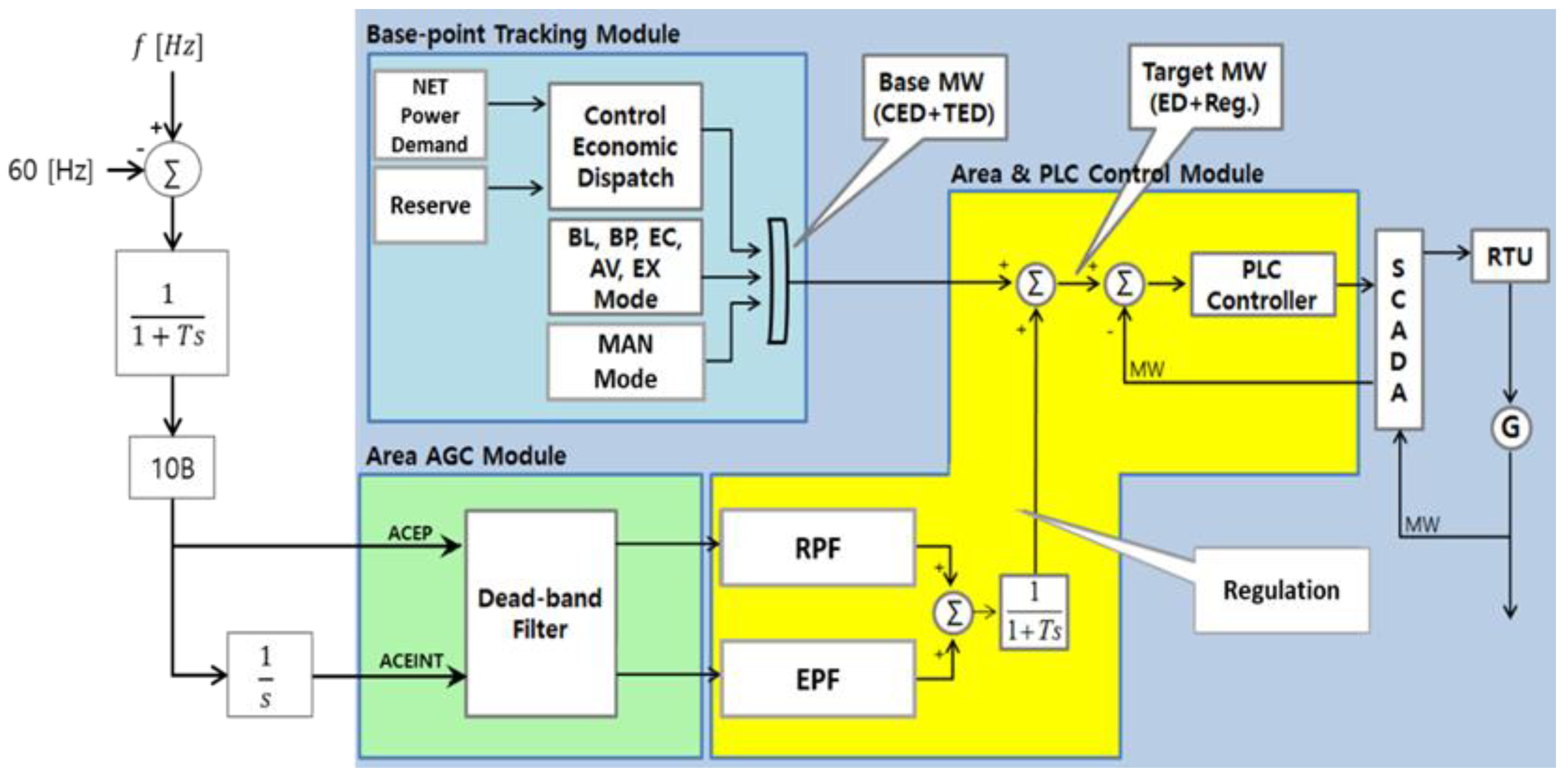
Figure 1 shows an overview of the AGC frequency control of the Korean power system, as illustrated in Reference [
6].
As shown in
Figure 1, the AGC frequency control of the Korean power system is performed by the EMS. The system frequency is sampled every two seconds via supervisory control and data acquisition (SCADA) and is filtered through a low-pass filter (LPF), which softens out rapid frequency variations. Then, the area control error (ACE) is calculated using the filtered frequency according to Equation (1):
where
FA and
FS are the measured system frequency and nominal system frequency (60 Hz), respectively.
B is the frequency bias in MW/0.1 Hz, and it was set to 913 MW/0.1 Hz in 2019.
TE is the time error.
Thus, the ACE is the index of imbalance between the generators and loads in the power system. In this context, as the frequent activation of AGC frequency control under normal operating conditions affects the wear and tear of the generator, the AGC frequency control should not respond to instantaneous random variation. Moreover, as AGC should not conflict with the governor response under transient operating conditions, the AGC frequency control should respond slowly [
7]. Thus, AGC must be filtered or delayed using the LPF or ACE processing algorithm to protect equipment, and it should be coordinated with the governor response. The AGC should be able to make this coordinating operation by tuning its control parameters, and such a required characteristic of AGC is defined as the flexibility of AGC frequency control in this section. In order to do this, the ACE is generally processed in various ways depending on the control philosophy of the utility or country [
8]. For the Korean power system, the Korean control philosophy was reflected in the deadband filter to operate the AGC frequency control flexibly [
9]. The dynamic deadband filter is described in the next section in detail.
Then, the ACE adjusted using the dynamic deadband filter distributes the required MW power to each generator. In this context, the adjusted ACE is derived from the proportional and integral components. The proportional component of the ACE is ACEP and is calculated by using Equation (1). The integral component of the ACE is ACEINT and accumulates the system frequency deviation over time. Its calculation can be described by Equation (2):
ACEINTpre and ACEINTpro are the previous value of ACE integrated value and the current value of ACE integrated value, respectively. The AGC cycle is the calculating time for ACE and it was set to two seconds in the Korean power system.
That is, the proportional component of the ACE is distributed to each generator considering its ramp rate (ramping power factor, RPF), and the integral component of the ACE is distributed considering its generating unit price (economic power factor, EPF). The required MW power of each generator is filtered through an LPF.
The AGC signal sends the economic dispatch (ED) and the MW power required for each generator to maintain the desired frequency through SCADA to the PLC of the generators every four seconds. The ED is calculated every five minutes.
2.2. Deadband Filter of AGC Frequency Control
In the Korean power system, the deadband filter has been used to implement the flexibility of AGC frequency control [
9]. The main function of the deadband filter is to delay ACE activation by using the dynamic deadband and regulate its amount by applying different gains depending on system operating condition when the frequency drops in the power system.
Figure 2 depicts a detailed overview of the dynamic deadband filter.
As shown in
Figure 2, the control mode of the dynamic deadband filter is classified into deadbands (D), normal (N), assist (A), and emergency (E), depending on the magnitude of the calculated ACE. The first of the above categories consists of static and dynamic deadbands [
10]. As the calculated value of ACE increases, the control mode is changed to N, A, and E mode, and accordingly, the response of the generators according to the AGC frequency control is increased by increasing the size of the control gain multiplied by the ACE. The control mode is determined at every time-step depending on the amount of calculated ACE.
When the calculated ACE is smaller than the static deadband, ACE is not activated. However, ACE does not get activated due to the effect of the dynamic deadband even though the calculated ACE exceeds the static deadband. Thus, the gains of either the static or dynamic deadband make the value of ACE zero.
If the frequency is still not recovered to the expected frequency, the dynamic deadband starts decreasing in order to approach the static deadband at a rate of time. When the ACE exceeds the decreasing dynamic deadband, it is activated by applying the gain of the control mode. At this instant, the gains are applied differently depending on the control mode. Once the frequency is recovered and its ACE is smaller than the static deadband, the dynamic deadband is initialized and the ACE is not activated.
2.3. Coordination of Governor Response and AGC
The ancillary service of the Korean power system has recently amended the market rules to ensure that the power system operates with safety and security with the increasing penetration level of RES, as depicted in References [
4,
11].
Figure 3 shows the concept of the amended ancillary service.
In
Figure 3, the frequency regulation reserve, which was obtained by integrating the governor response and AGC frequency control, is classified as a frequency control reserve of 700 MW for normal operating conditions and a frequency recovery reserve for transient operating conditions. The frequency recovery reserve is subdivided into a primary reserve of 1000 MW, a secondary reserve of 1400 MW, and a tertiary reserve of 1400 MW.
The primary reserve of the Korean power system is activated by the governor of the generator, except for the nuclear power plant. When a large-scale generator trips in the Korean power system, the primary reserve secured by 1000 MW must be activated within 10 s and last for at least 5 min to maintain the frequency decrease. In this case, the system frequency is maintained at a frequency of 59.7 Hz and is restored above 59.8 Hz within 1 min.
The frequency control reserve generally called “AGC” activates the system frequency to smooth out the variability of load under normal operating conditions. In addition, the frequency control reserve secured by 700 MW must be activated within 5 min and last for at least 30 min. The secondary reserve is also called “AGC” but is used only for contingency. This is responsible for backing up the primary reserve. It must be activated within 10 min and last for at least 30 min following the event of a generator trip in the Korean power system. Furthermore, the secondary reserve of the Korean power system must be secured by 1400 MW.
Thus, the interaction between the governor response and the AGC frequency control was clarified by the amended ancillary service concept. Consequently, it becomes important to coordinate these services with each other.
3. Dynamic Simulation Model of AGC
The dynamic-model-based simulation frameworks, which are typically used for power system analysis by the utilities, are adapted to include the AGC frequency control to implement the simulation model for both the AGC and governor responses. As the database of the Korean power system has been implemented in the framework of PSS/E, Python is used as its application program interface (API) for implementing the AGC frequency control and interfacing its responses to the dynamic-model-based simulation using PSS/E. Accordingly, the proposed simulation model can flexibly implement the AGC frequency control and effectively use the existing models of power systems. This section describes the details of the proposed simulation model by dividing it into a system aspect implementing the AGC operation and a generator aspect linking it to dynamic simulation.
3.1. Dynamic-Model-Based Implementation of Load Frequency Control in the Korean Power System
As AGC controls the power system frequency by adjusting the generation targets of centrally dispatched generators based on the frequency deviations, its simulation model should be able to calculate the corresponding amount of LFC required by the disturbance and allocate it to each generator. The operational mechanism of the AGC frequency control is implemented in Python, which is an API program of PSS/E where the dynamic data of the Korean power system have been managed, for the flexibility and compatibility of the proposed simulation model [
12,
13,
14,
15].
In addition, the proposed model uses an existing program, such as PSS/E, as a solver of the power system with the responses of the generators assigned by the AGC frequency control. As the dynamic characteristics of the power system are simulated in solving the power system using the dynamic-model-based program PSS/E, the proposed model can determine the response of the power system to the AGC frequency control considering the dynamics of the power system.
Figure 4 shows the simulation framework of the dynamic-model-based AGC frequency control.
As shown in
Figure 4, in every AGC cycle, Python API runs the dynamic simulation of the power system with the given data by calling the PSS/E program and performs AGC frequency control using the simulated operation results. By repeating this process, the proposed model can simulate the AGC frequency control based on the dynamic model of the power system.
Figure 5 shows the process of simulation for the AGC frequency control using Python.
As shown in
Figure 5, the proposed model calculates ACEP and ACEI using the dynamic-model-based simulation method at every AGC cycle. The calculated ACEP and ACEI are adjusted by applying the dynamic deadband filter and then assigning the response to the generators. Finally, the dynamics of the power system are simulated using the responses of the generators to the assigned AGC targets.
3.2. Modeling of Generators for Simulating AGC
As the existing dynamic models of generators have been implemented to simulate the dynamic responses of the generators themselves, these models need to be modified to receive and process the AGC command for those outputs in the proposed simulation framework. In the operating system in the field, each generator takes the AGC signal via PLC, as illustrated in Reference [
16]. The role of PLC is to adjust the AGC target for coordination with the governor response [
3]. For instance, consider a case where the governor of each generator orders an increase in its power output immediately after the frequency drop caused by a contingency, but the AGC target is not changed from the previous command at this time due to the AGC updating cycle. Consequently, each generator would not be able to provide the primary frequency response. Therefore, the PLC is used to adjust the AGC target when the governor responds to the disturbance so that the response can be sustained.
In the proposed simulation framework, the PLC functions are implemented in the existing dynamic models of generators. In the Korean power system, the mainly used models for governors are GGOV1, GAST TGOV1, and IEEEG1. In the case of the GGOV1 model, the interfacing AGC command with the matched input of the GGOV1 model would be able to implement the PLC function, as shown in
Figure 6.
As shown in
Figure 6, the implementation of the PLC function of the GGOV1 model is indicated by a red circle. Upon sending the AGC target to the Pmwset of the GGOV1 model through Python-API, the GGOV1 model responds to the AGC frequency control in coordination with the governor response.
In the case of the remaining models, the LCFB1 model which is a standard turbine load controller model for the governor in PSS/E program is added to implement the PLC function for linking the AGC command to the governor, as shown in
Figure 7,
Figure 8 and
Figure 9.
As shown in
Figure 7,
Figure 8 and
Figure 9, the added LCFB1 model revises the AGC target with the amount of difference between the received AGC target and the actual power output of the generator.
In the proposed simulation model, by feeding the revised AGC target from the LCFB1 model to the governor model as its output reference, the PLC function for the coordination between the AGC frequency control and the governor response immediately after the disturbance is implemented.
4. Case Study
In this section, the effectiveness of the proposed method is verified through case studies employing the Korean power system. As the Korean power system does not have any interconnection with neighboring countries, its frequency control is controlled only by its own operating reserves, including the governor responses and AGC frequency controls. However, their effective operation has increasingly become a concern with the increasing penetration level of RES.
The dynamic data of the Korean power system are obtained from the planning database of the power utility [
17], which is maintained in the format of PSS/E. The operating conditions of the power system are assumed to be a set of typical values used in the planning database, where the total electricity demand is 94 GW, provided by 276 generators. Among the 276 generators, all the generators except for 27 nuclear generators provided the governor response, and 143 generators provided the AGC frequency control.
4.1. Verifocation of the Simulation Model for AGC Frequency Control
This case study reviewed each process function of the simulation for the AGC frequency control according to
Figure 5 to verify the effectiveness of the proposed simulation model.
Figure 10 shows the filtered frequency, which is used to calculate the ACE in the proposed model assuming a generator trip.
An efficient and stable response of the AGC frequency control can be achieved by using the filtered frequency for calculating the ACE.
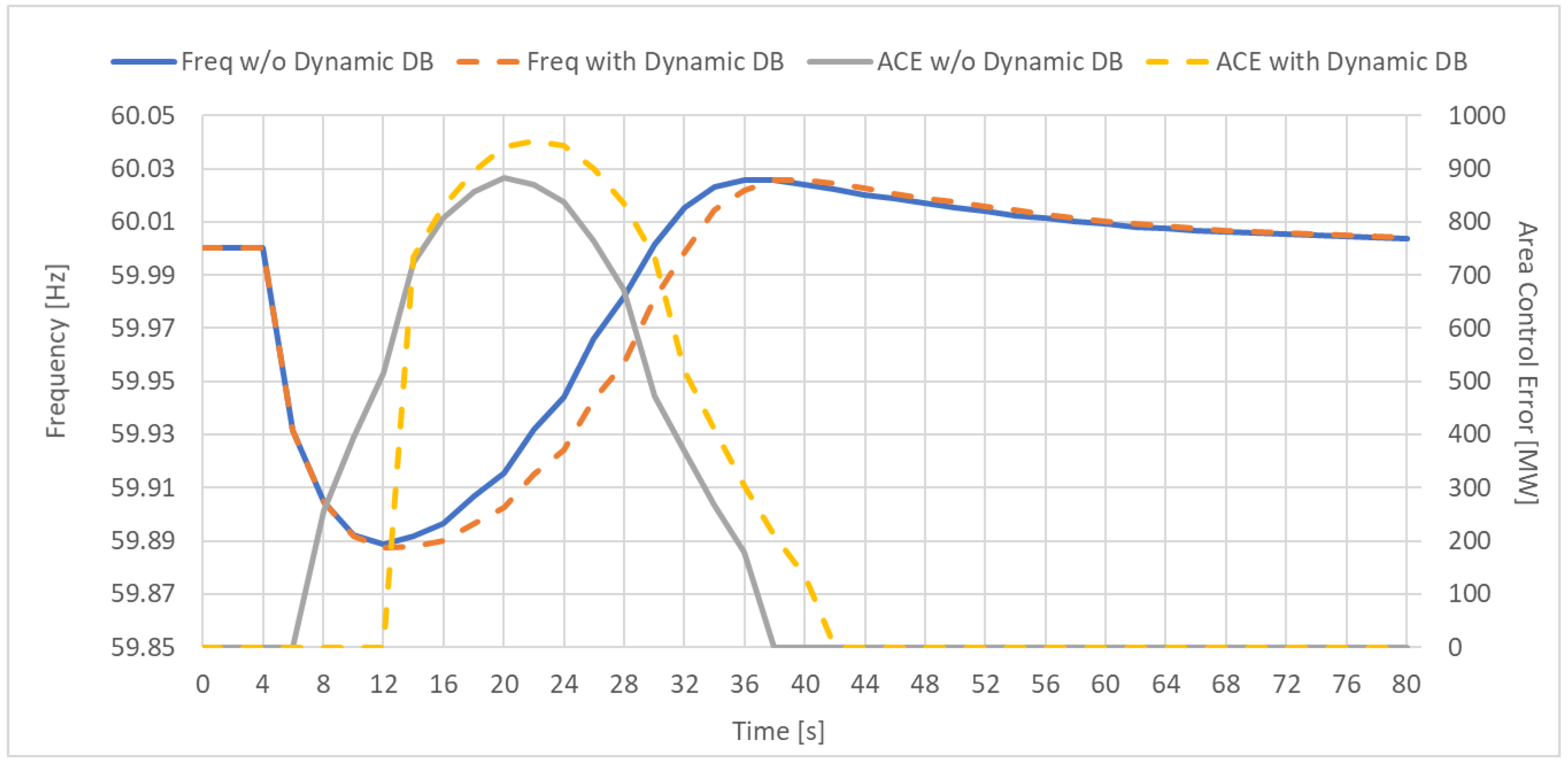
The function of the dynamic deadband is verified by comparing the operating results of the AGC frequency control with and without it.
Figure 11 shows the simulation results for the comparison in terms of the ACE and controlled frequency.
As shown in
Figure 11, the dynamic deadband delays the activation of the ACE when the frequency drops. However, the performance of the frequency control is not deteriorated by the delayed activation of the ACE because the nadir of the controlled frequency is the same as that in the case where the ACE is instantly activated without the dynamic deadband. Therefore, it would be efficient to operate the AGC frequency control with some degree of delay by using the dynamic deadband during a transient period, as even an instant response of the AGC frequency control would not be able to contribute to the frequency control owing to the overlap with the governor responses immediately after the disturbance. The detailed simulation results of the proposed model are shown in
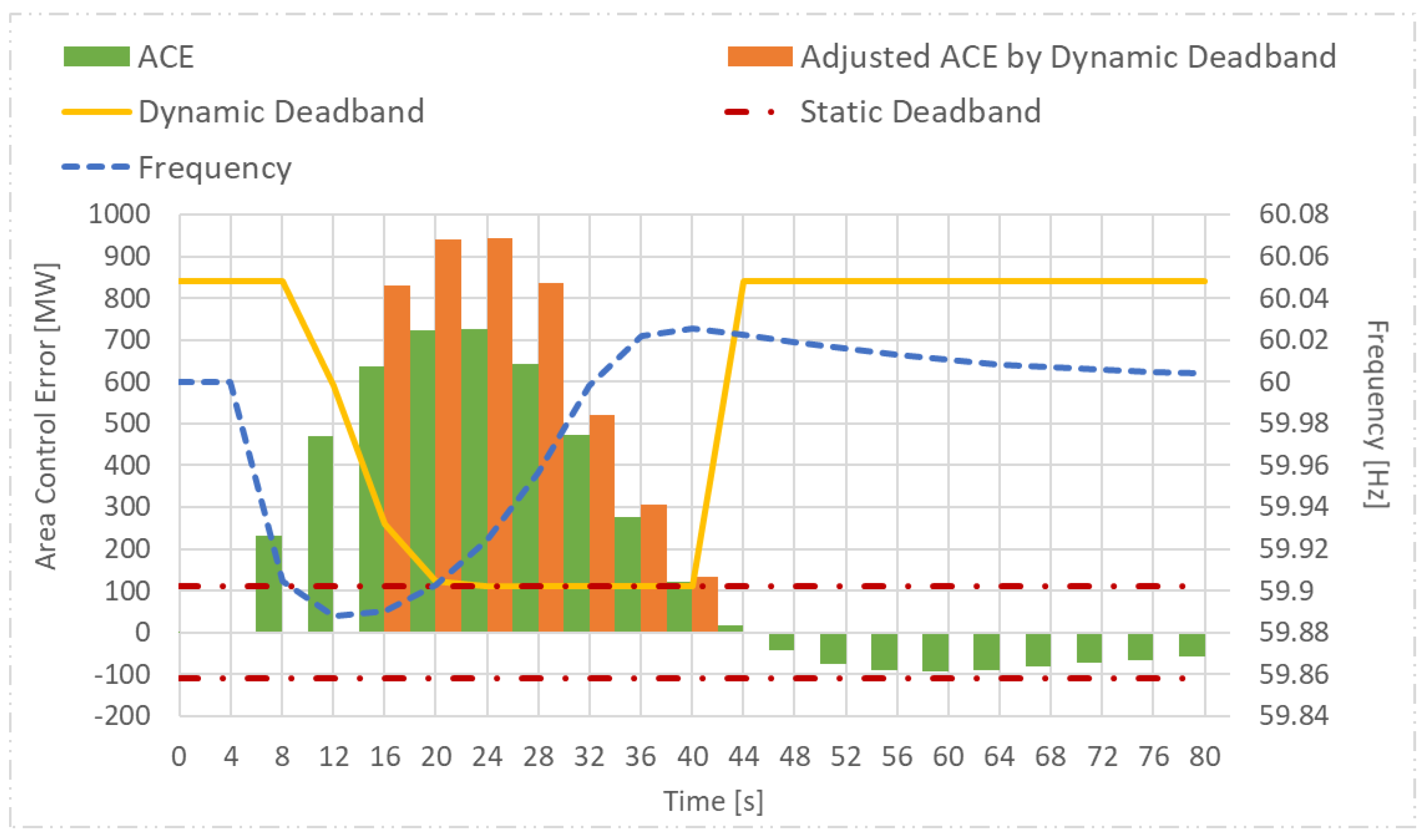
Figure 12.
As illustrated in
Figure 12, the ACE is not activated immediately after the frequency drop because of the dynamic deadband. However, if the frequency is not recovered until its ACE exceeds the decreasing dynamic deadband, the ACE is activated and its amount is adjusted by the control gain depending on the control mode. Once the frequency is recovered and its ACE is smaller than the static deadband, the dynamic deadband is initialized. The activated ACE is allocated to each generator as the AGC frequency control target.
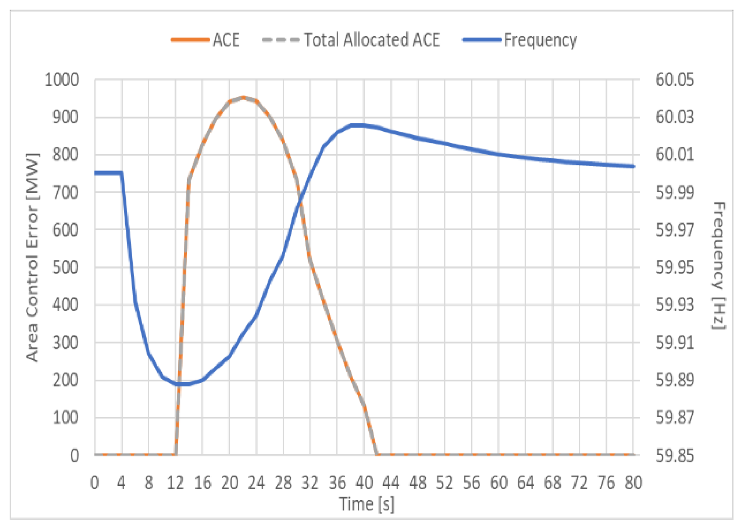
Figure 13 shows an example of ACE allocation using the proposed simulation model.
As shown in
Figure 13, the amount of activated ACE depends on the frequency drop, and it is allocated to each generator using the proposed simulation model.
In the AGC frequency control operation, the allocated ACE is received by each generator through its PLC so that the governor response could be prioritized in the frequency control. In this study, the PLC of the proposed model is verified by applying the contingency of the generator trip.
Figure 14 illustrates the simulation results of the PLC function.
As illustrated in
Figure 14, once the measured output of the generator is different from the received AGC target, the PLC is activated to revise the received AGC target by adding a governor response to it. Therefore, the output of the generator follows the revised AGC target rather than the received target.
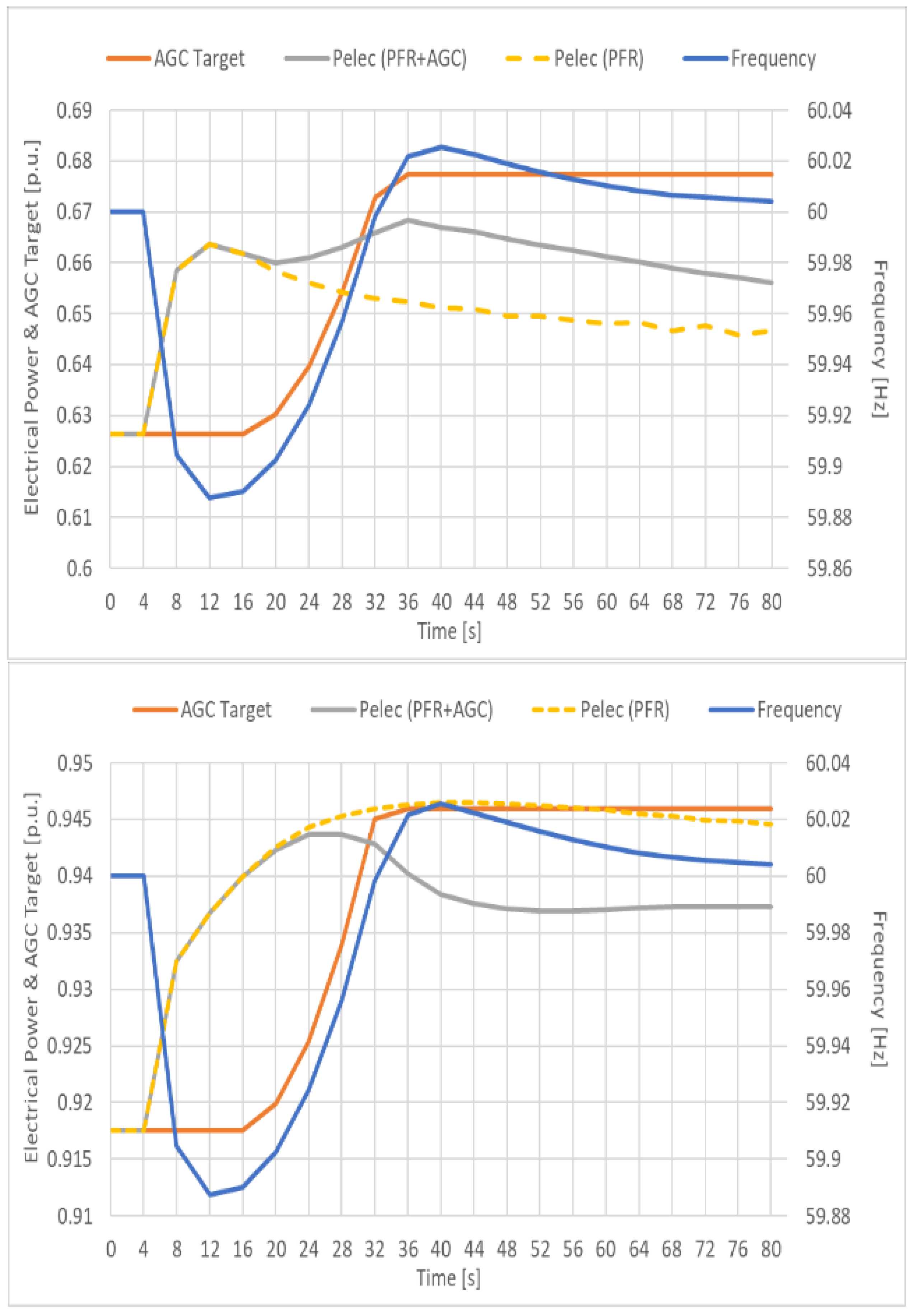
Once the AGC target is received by each generator, it should be met with a response from the generator even considering its PLC function. The performance of the proposed simulation model is verified by comparing the output of the generator and the AGC target in terms of the appropriateness of the AGC allocation and generator dynamics.
Figure 15 shows the AGC response of the generators with the highest and lowest amounts of ACE allocation.
As shown in
Figure 15, the amount of ACE allocated to GEN#1 is smaller than that allocated to GEN#2. This is because GEN#1, a coal generator, has a lower performance than GEN#2, a gas generator. As the output of the generators could satisfy the revised AGC target, the appropriateness of the AGC allocation could be verified by considering the dynamics of the two generators.
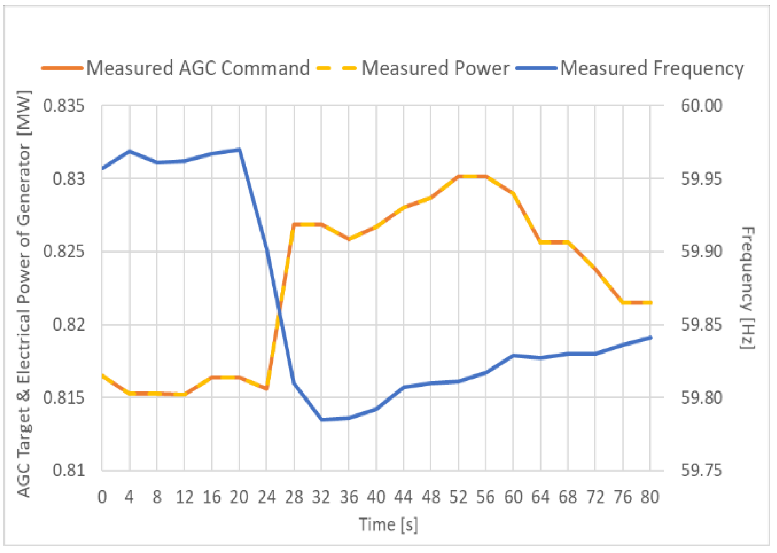
To validate the proposed model, the simulated results are also compared by the selected actual frequency responses in the Korean power system. The real-event data was recorded when a nuclear generator of 1 GW tripped in 2013. Since there must be differences in the detailed operating conditions of the real event and the simulated case, those should be compared only in terms of AGC frequency control.
Figure 16 compares ACE calculations of the measured and simulated case to the same frequency recorded in the real case.
As shown in
Figure 16, the simulated ACE was matched with the measured ACE and this validates that the proposed model could be used to simulate real ACE calculations by appropriately setting the control parameters.
In addition, AGC command dispatched to a specific generator and its response is compared using the same event as shown in
Figure 17.
As shown in
Figure 17, the time delay in the AGC activation that occurred in the measured data could be also found in the simulated results. This validates that the proposed model could simulate the time response of the real AGC operation.
4.2. Analysis of Tuning AGC Frequency Control
In this section, case studies using the proposed simulation model for analyzing the effects of setting the deadband filter of the AGC frequency control, which should consider both the dynamics and AGC operation of the power system, are described. As the proposed model simulates the frequency performance of the power system synthesizing the governor response and AGC operation, the effect of parameter setting can be analyzed by considering not only the effect of the parameter itself but also the coordination with the governor response.
The deadband filter has three control parameters: variable time, the boundary of the control mode, and the control gain at each mode. The variable time delays the activation of the AGC frequency control for coordination with the governor response.
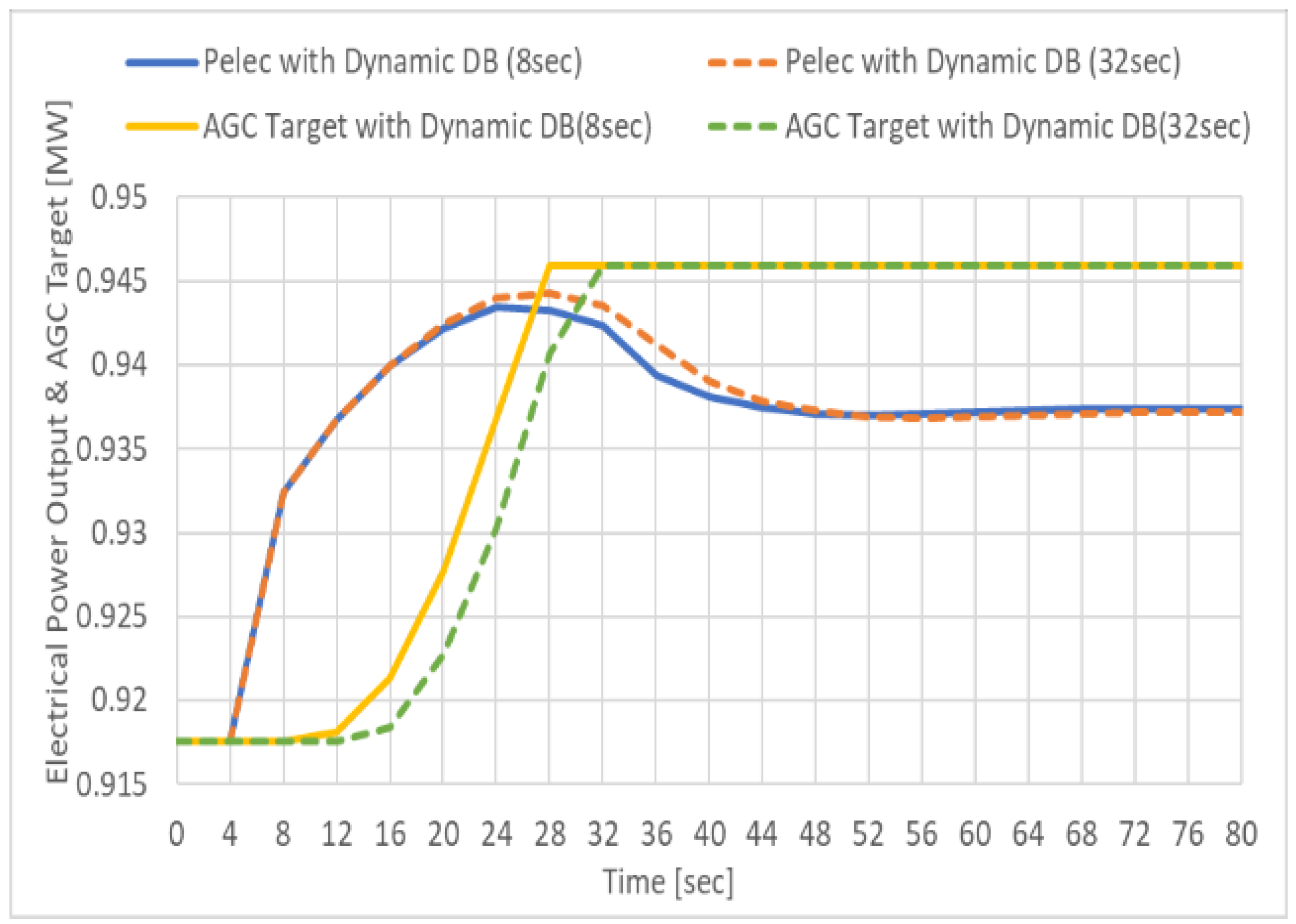
Figure 18 illustrates the simulation results of the frequency control with different variable times of the deadband filter in the AGC operation.
As shown in
Figure 18, the ACE activation time is controlled by the variable time of the dynamic deadband, and it affects the frequency response of the generators and the frequency of the power systems. Although the frequency recovered faster when the variable time of the dynamic deadband was reduced from 32 to 8 s, the AGC frequency control could not improve the nadir frequency. This appears to be because the generator power was saturated with the governor response, as shown in the lower figure in
Figure 18. Accordingly, the proposed model can be used to set the variable time of the dynamic deadband appropriately in AGC operations.
The boundary conditions of the control modes are used to determine the status of the power system depending on the amount of ACE. In this case study, three cases are assumed for the proposed simulation model with different sets of boundary conditions, as summarized in
Table 1. As one goes from cases 1 to 3, the range of each mode becomes wider and the emergency mode appears later. For analyzing the effectiveness of boundary conditions of the control modes only, the variable time of the dynamic deadband is set as 32 s, and the control gains are set as 1.0 in all three cases.
Figure 19 shows the simulation results using the proposed model for the three cases and the distribution of the control mode determined every 2 s during the simulation.
As shown in
Figure 19, the activation of the AGC frequency control is also delayed by setting the ranges of the control modes wider. Among the three cases, the boundary condition of case 2 appears to be relatively more reasonable considering the frequency drop because the frequency could recover earlier without the emergency mode. In the case of 1, the nadir frequency could not be improved even by the more frequent emergency modes.
Accordingly, the proposed model can be used to set the boundary conditions of the control modes appropriately in the AGC operations. It can also be observed from
Figure 19 that the nadir frequency is the same in all three sets of boundary conditions, but the frequency recovers earlier with narrower ranges of the control modes.
The control gain of each mode determines the strength of the AGC frequency control. In this study, three cases are assumed with different sets of proportional control gains, as summarized in
Table 2 where the boundary conditions of the control modes are assumed to be the same as those in case 2 of
Table 1. As one goes from cases 1 to 3 in
Table 2, the proportional control gain of each mode increases. The boundary conditions of the control modes are assumed to be the same as those in case 2 of
Table 1.
Figure 20 shows the simulation results using the proposed model for these three cases.
As shown in
Figure 20, the frequency recovers faster with higher control gains of the AGC frequency control. However, the high control gain in the AGC frequency operation can cause an overshoot of the power system control. Accordingly, the proposed model can be used to set the control gains of each mode appropriately in the AGC operations.
As shown in the results of the case studies, the proposed simulation model can be used to tune the control parameters of the AGC frequency control considering both the dynamics and AGC operations of the power system. This is one of the benefits of developing a simulation model for the AGC frequency control based on the dynamic models of the power systems.
5. Conclusions
This paper proposed a dynamic-model-based AGC frequency control simulation method employing the Korean power system that can be designed and analyzed coordinately with the governor responses of the generators. The existing dynamic-model-based simulation frameworks typically used for power system analysis were adapted to include the AGC frequency control to implement the simulation model for both the AGC frequency control and governor responses. As the database of the Korean power system has been implemented in the framework of PSS/E, Python was used as the API for implementing the AGC frequency control and interfacing its responses to the dynamic-model-based simulation model through additional PLC functions of the governor models using PSS/E. Accordingly, the proposed simulation model could flexibly implement the AGC frequency control and effectively use the existing models of power systems.
The effectiveness and applicability of the proposed simulation model for AGC frequency control were verified using various case studies. These case studies examined each function of the AGC frequency control and analyzed the effects of variation of the control parameters related to the deadband filter of the AGC frequency control.
Owing to the need to operate the power system more competitively with more variable resources, the proposed simulation model can be used to tune the control parameters of the AGC frequency control to achieve a highly efficient coordination of operations with the governor responses from local generators.
Author Contributions
Conceptualization, H.N.G. and K.S.K.; methodology, H.N.G. and K.S.K.; software, H.N.G.; validation, H.N.G., and K.S.K.; writing-original draft preparation, H.N.G. and K.S.K.; writing-review and editing, K.S.K.; supervision, K.S.K. All authors have read and agreed to the published version of the manuscript.
Acknowledgments
This research was partially supported by the Korea Electric Power Corporation (grant number: R18XA04).
Conflicts of Interest
The authors declare no conflict of interest.
References
- Korean Ministry of Trade, Industry and Energy. The 8th Basic Plan for Long-Term Electricity Supply and Demand (2017–2031); Korean Misnistry of Trade, Industry and Energy: Sejong, Korea, 2017.
- Hector, C.; Ross, B.; Julija, M. The joint adequacy of AGC and primary frequency response in single balancing authority systems. IEEE Trans. Sustain. Energy 2015, 6, 959–966. [Google Scholar]
- NERC. Reliability Guideline: Primary Frequency Control; NERC: Washington, DC, USA, 2015. [Google Scholar]
- Wood, A.J.; Wollenberg, B.F. Power Generation Operation and Control, 2nd ed.; John. Wiley & Sons: New York, NY, USA, 1996. [Google Scholar]
- Korea Power Exchange (KPX). Electricity Market and Power System Operating Guide; Korea Power Exchange (KPX): Naju, Korea, 2019; p. 278. [Google Scholar]
- Choi, Y.M.; Lee, G.W. Introduction of EMS AGC Group Control. In Proceedings of the KIEE 2008 Power Engineering Society Fall Conference and General Meeting; pp. 133–135. Available online: http://www.dbpia.co.kr/journal/articleDetail?nodeId=NODE01336617 (accessed on 25 September 2020).
- Choi, S.H.; Hwang, K.I.; Chun, Y. Evaluation of AGC characteristics and a novel AGC control strategy for independent power systems. Trans. Korean Inst. Electr. Eng. A 2005, 54, 540–547. [Google Scholar]
- Unbenhauen, H.D. Automation and Control of Electrical Power Generation and Transmission Systems. In Control Systems, Robotics and Automation–Volume: Industrial Applications of Control Systems; EOLSS Publishers Co. Ltd.: Oxford, UK, 2009; Volume 18, p. 213. [Google Scholar]
- Korea Power Exchange (KPX) & Jeonbuk National University (JBNU). A Study on Optimal Perform Method of AGC and Criteria Establishment for Control Variables; Korea Power Exchange (KPX): Naju, Korea, 2014. [Google Scholar]
- Chang Soo, O.; Suk Ha, S.; Woon Hee, L. Optimal AGC Control Parameter Tuning. In Proceedings of the KIEE 2008 Power Engineering Society Fall Conference and General Meeting; pp. 321–322. Available online: https://www.koreascience.or.kr/article/CFKO200814835315828.pdf (accessed on 25 September 2020).
- Korea Power Exchange (KPX). Decree on Reliability Standard and Electricity Quality; Korea Power Exchange (KPX): Naju, Korea, 2019. [Google Scholar]
- Siemens PTI. PSS/E 34 Application Program Interface (API); SIEMENS: New York, NY, USA, 2015. [Google Scholar]
- Wang, L.; Chen, D. Experience with Automatic Generation Control (AGC) Dynamic Simulation in PSS/E. Power Technol. 2012. Available online: https://static.dc.siemens.com/datapool/us/SmartGrid/docs/pti/2012August/PDFs/Experience_on_AGC_Dynamic_Simulation_in_PSSE.pdf (accessed on 25 September 2020).
- Wang, L.; Chen, D. Automatic Generation Control (AGC) Dynamic Simulation in PSS/E. Power Technol. 2011. Available online: https://static.dc.siemens.com/datapool/us/SmartGrid/docs/pti/2011February/PDFs/AGC%20Dynamic%20Simulation%20in%20PSSE.pdf (accessed on 25 September 2020).
- Siemens PTI. PSS/E 34 Model Library; SIEMENS: New York, NY, USA, 2015. [Google Scholar]
- NERC. Reliability Guideline; Application Guide for Modeling Turbine-Governor and Active Power-Frequency Controls in Interconnection-Wide Stability Studies; NERC: Atlanta, GA, USA, 2019. [Google Scholar]
- Korea Power Exchange (KPX). Annual Operating Results of Korean Electricity Market in 2019; Korea Power Exchange: Seoul, Korea, 2020; p. 2. [Google Scholar]
Figure 1.
Automatic generation control (AGC) operation in the Korean power system.
Figure 1.
Automatic generation control (AGC) operation in the Korean power system.
Figure 2.
Concept of dynamic deadband in deadband filter.
Figure 2.
Concept of dynamic deadband in deadband filter.
Figure 3.
Concept of amended ancillary service in the Korean power system.
Figure 3.
Concept of amended ancillary service in the Korean power system.
Figure 4.
Simulation framework for AGC in the Korean power system.
Figure 4.
Simulation framework for AGC in the Korean power system.
Figure 5.
Simulation process of the AGC frequency control.
Figure 5.
Simulation process of the AGC frequency control.
Figure 6.
AGC interfacing with the GGOV1 model.
Figure 6.
AGC interfacing with the GGOV1 model.
Figure 7.
IEEEG1 model interfacing with the LCFB1 model for simulating AGC.
Figure 7.
IEEEG1 model interfacing with the LCFB1 model for simulating AGC.
Figure 8.
TGOV1 model interfacing with the LCFB1 model for simulating AGC.
Figure 8.
TGOV1 model interfacing with the LCFB1 model for simulating AGC.
Figure 9.
GAST model interfacing with the LCFB1 model for simulating AGC.
Figure 9.
GAST model interfacing with the LCFB1 model for simulating AGC.
Figure 10.
Comparison of frequency and filtered frequency using low-pass filter.
Figure 10.
Comparison of frequency and filtered frequency using low-pass filter.
Figure 11.
AGC frequency control with and without dynamic deadband.
Figure 11.
AGC frequency control with and without dynamic deadband.
Figure 12.
Verification of dynamic deadband activation.
Figure 12.
Verification of dynamic deadband activation.
Figure 13.
Example of area control error allocation using the proposed simulation model (upper) and comparison of between the total allocated area control error and pre-allocated area control error (lower).
Figure 13.
Example of area control error allocation using the proposed simulation model (upper) and comparison of between the total allocated area control error and pre-allocated area control error (lower).
Figure 14.
Revised AGC target by the plant-level controller function.
Figure 14.
Revised AGC target by the plant-level controller function.
Figure 15.
AGC frequency control response of GEN#1 (upper) and GEN#2 (lower).
Figure 15.
AGC frequency control response of GEN#1 (upper) and GEN#2 (lower).
Figure 16.
Comparison of the measured and the simulated ACE.
Figure 16.
Comparison of the measured and the simulated ACE.
Figure 17.
Comparison of the AGC activation time between the measured (upper) and simulated (lower).
Figure 17.
Comparison of the AGC activation time between the measured (upper) and simulated (lower).
Figure 18.
The area control error activation time (upper) and the frequency response of generator (lower) depending on variable times of the dynamic deadband.
Figure 18.
The area control error activation time (upper) and the frequency response of generator (lower) depending on variable times of the dynamic deadband.
Figure 19.
Comparison of frequency response with different bounds of control mode (upper) and the distribution of the determined control mode (lower).
Figure 19.
Comparison of frequency response with different bounds of control mode (upper) and the distribution of the determined control mode (lower).
Figure 20.
Comparison of frequency responses with different control gains.
Figure 20.
Comparison of frequency responses with different control gains.
Table 1.
Bounds of the control mode (ACE: Area Control Error; Static DB: Static Deadband).
Table 1.
Bounds of the control mode (ACE: Area Control Error; Static DB: Static Deadband).
| Cases | Static DB | Normal | Assist | Emergency |
|---|
| Case 1 | | | | |
| Case 2 | | | | |
| Case 3 | | | | |
Table 2.
Gain setting of each control mode.
Table 2.
Gain setting of each control mode.
| Cases | Normal | Assist | Emergency |
|---|
| Case 2.1 | 0.1 | 0.3 | 0.5 |
| Case 2.2 | 1.1 | 1.3 | 1.5 |
| Case 2.3 | 2.1 | 2.3 | 2.5 |
© 2020 by the authors. Licensee MDPI, Basel, Switzerland. This article is an open access article distributed under the terms and conditions of the Creative Commons Attribution (CC BY) license (http://creativecommons.org/licenses/by/4.0/).


