Saturation Modeling of Gas Hydrate Using Machine Learning with X-Ray CT Images

Abstract

This study conducts saturation modeling in a gas hydrate (GH) sand sample with X-ray CT images using the following machine learning algorithms: random forest (RF), convolutional neural network (CNN), and support vector machine (SVM). The RF yields the best prediction performance for water, gas, and GH saturation in the samples among the three methods. The CNN and SVM also exhibit sufficient performances under the restricted conditions, but require improvements to their reliability and overall prediction performance. Furthermore, the RF yields the lowest mean square error and highest correlation coefficient between the original and predicted datasets. Although the GH CT images aid in approximately understanding how fluids act in a GH sample, difficulties were encountered in accurately understanding the behavior of GH in a GH sample during the experiments owing to limited physical conditions. Therefore, the proposed saturation modeling method can aid in understanding the behavior of GH in a GH sample in real-time with the use of an appropriate machine learning method. Furthermore, highly accurate descriptions of each saturation, obtained from the proposed method, lead to an accurate resource evaluation and well-guided optimal depressurization for a target GH field production.

1. Introduction

Previous studies, in the field of petroleum engineering, have performed core experiments to understand how multi-phase fluids flow through porous media and measure important petrophysical features, such as permeability or porosity [1,2,3,4,5]. Mass balance can be used to analyze changes in saturation and pressure in each phase during a core experiment. This requires the entire core to be acting as a single system, under the assumption that the attributes of the target core have homogeneous characteristics. In addition, changes in the saturation or its trend can be indirectly analyzed depending on observations of the pressure, temperature, and fluid injection/production in conventional core flow experiments. Although the saturation presents an overall change throughout the entire core system based on the mass balance equation, there is a lack of understanding with respect to the behavior of every single spot in a sample.

In particular, characteristics of gas hydrate (GH) distribution is strongly heterogeneous and stochastic behavior during its formation and dissociation. To analyze production behavior in unconsolidated sand, previous studies have conducted mass balances using water and gas production, measured during the GH dissociation. However, a certain amount of error was present due to the time gap between when dissociation occurs and when the dissociated water and gas rates are measured. Besides, even if it has the same experimental condition, the characteristics of the production behavior may appear differently owing to the existence of dead volume accumulation or free gas [6,7,8]. Therefore, previous studies had difficulties in describing the behavior and saturation of multiple phases in GH. Therefore, we must introduce a non-destructive inspection method for the directional and quantitative analysis of the behavior of GH inside a cell in real-time. To solve this issue, medical X-ray CT (computerized tomography) was proposed in previous studies [6,7,8,9,10] to understand the heterogeneity to obtain a more accurate description of GH behavior [11,12,13,14,15,16,17,18].

CT imaging has, therefore, been proposed to overcome problems associated with previous experiments and suggest improved trend descriptions for porous media. This technique can illustrate the distribution of each fluid phase. Furthermore, medical CT has numerous advantages, i.e., real-time analysis, a rapid scanning velocity, and other conveniences during experimentation that can be employed to understand the varying trends in the formation and dissociation of GH [6,8]. Despite this, there are certain limitations, where the given values of CT images only present mixed results owing to the saturation of all the phases and matrix caused by the low resolution of the medical CT technique. Therefore, CT imaging cannot identify the saturation of each phase. In particular, there is a difficulty in segmentation between water and GH owing to their similar densities. Therefore, we must model and predict the saturation of each phase from the CT images, which can lead to improved interpretations and comprehension of GH experiments, as well as more reliable numerical simulations of GH.

Recent studies have widely applied machine learning (ML) algorithms to a variety of field data types in the domain of petroleum exploration and production [19]. These studies attempt to propose suitable pre-processing procedures and ML algorithms depending on the given data types and domain knowledge. For example, a recurrent neural network (RNN) was used for time-series data (e.g., production history) [20], while the convolutional neural network (CNN) was used for image data (e.g., seismic amplitude) [21,22]. For core experimental data, segmentation algorithms, such as U-net, were used to distinguish specific objects in high-resolution images [23,24,25].

To the best of our knowledge, no previous studies have addressed the problem of saturation modeling in GH sand sample images. In this study, we examine the appropriate pre-processing procedures and ML algorithms that can be used in the case of experimental CT data related to GH samples.

2. Methodology

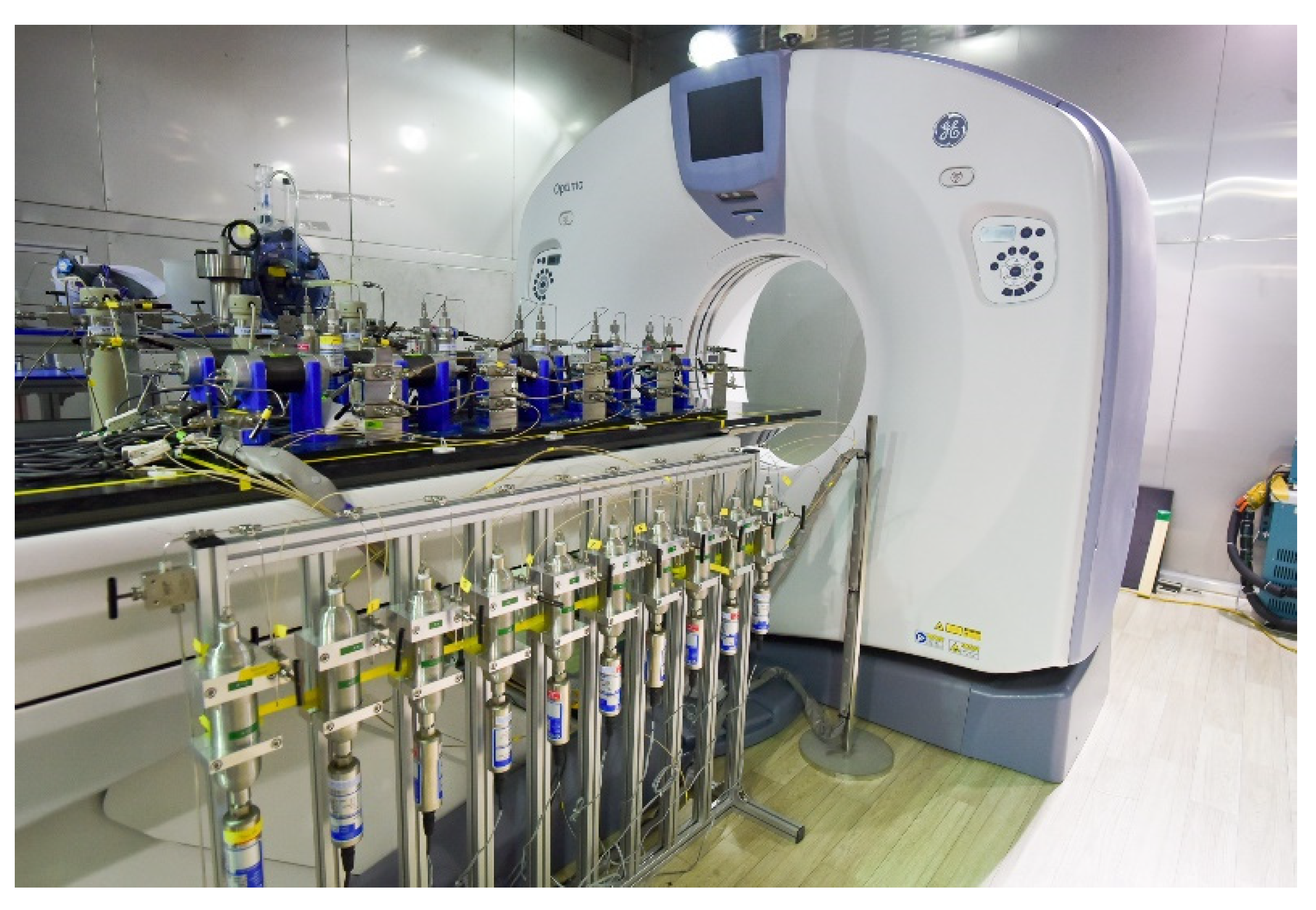
2.1. GH Experiment with CT Imaging

The visualization system with the X-ray CT is composed of five main components in this study: sample installation, fluid injection, fluid production, control and measurement of the data, and X-ray CT (Figure 1 and Figure 2). The sample installation component consists of a high-pressure cell, temperature control for the high-pressure cell, and measurement equipment for the temperature and pressure of the cell. The high-pressure cell is cylinder-shaped, with an inner diameter and length of 1 and 2 inches, respectively. The cell is made from a strengthened glass fiber and aluminum complex to increase the transmissivity of the X-rays and stability from high pressure condition at ~20 MPa. “Porous media” is installed to minimize and prevent leaks in the unconsolidated sand sample in the inlet and outlet of the cell. In addition, an air-cooler is equipped near the high-pressure cell to maintain the temperature where the system generates the GH. Near the inlet and outlet, a resistance temperature detector type thermometer and DXD digital output pressure transducer (3000 psi) are applied, respectively. The fluid injection component injects water and methane gas for GH formation. A syringe pump (500D Syringe Pump manufactured by Teledyne ISCO) and mass flow controller (model SLA5850S manufactured by BrooksInstrument) were used to input water and gas, respectively. The fluid production component connects to the back pressure regulator (BPR) and syringe pump to control the pressure of the BPR. Water and gas are drained at the same time during GH dissociation. Thus, the fluid production component consists of a separator for the water and methane, mass balance meter, and wet gas meter (model TG0.5 manufactured by Ritter). The control component manage the syringe pump and mass flow controller. The measurement component gauges the temperature, pressure, and rates of the water and gas in real-time. The X-ray CT is taken with medical grade CT equipment (model OPTIMA 660 manufactured by General Electricity), which is characterized by a fast-filming velocity (96 mm/s). The CT was used for visualization and analysis of the phase behavior in the high-pressure cell in real-time. The CT system was installed in a chamber that shields the radioactivity, such that we were able to control the temperature and humidity and obtain CT images in a stable environment.

The pressure of a sample is charged by methane, followed by a decrease in the temperature until the GH is formed at low temperature-high pressure conditions. These procedures are conducted throughout the five stages of the experiment. CT images are obtained in each stage to perform CT normalization analysis and build training data for the machine learning methods.

First, the sample is packed with sand in the high-pressure cell. The used sample is a duplicate characterized by the same attributes as samples acquired from the Korean East Sea region, which is a promising area for GH resources. We obtained the charge of the sedimentary grain using a vibrator to homogeneously distribute the particles in a dry state. Additionally, the homogeneity of the grain was verified in the CT images during the charging process. In this study, the GH experiment was conducted three times. Therefore, there are three sets of samples names, A, B, and C, all of which have 35% porosity.

The packing procedure is the first procedure among the five experiment stages (Figure 3a), where the sample is scanned by the CT to obtain the image data. The high-pressure cell was then coupled with temperature and pressure sensor and water and gas line. The sample remained in a vacuum environment for more than six hours. The sample was saturated with 100% water, followed by CT scanning of the sample (Figure 3b). We can calculate the porosity of the sample by measuring the amount of injected water. Methane gas was injected into the sample and the initial water and gas saturation was set as “IWS,” as well as with CT scan (Figure 3c). At this sample condition, extra methane gas was injected to reach the high pressure condition, followed by a decrease in the temperature to form the GH (CT scan for GH shown in Figure 3d). Free gas in the pore was displaced via water injection to obtain similar conditions and environment as the research target area, i.e., the Korean East Sea. The “GTW” stage was scanned by CT (Figure 3e). The resolution of the acquired CT images was 512 × 512 × 96 for the three GH samples, A, B, and C, and the size of each pixel was ~100 and 660 $\mathsf{\mu }$m for the horizontal and vertical direction, respectively. High intensity CT value areas, such as the end-piece, which includes the temperature sensor, were excluded to obtain the proper CT values for machine learning.

If we assume that there is no particle movement in the sample, we can compute the normalized CT values [4,6,8,26]. All CT values from the five stages were normalized as follows:

$${\mathrm{CT}}_{norm}=\frac{{\mathrm{CT}}_{STAGE}-{\mathrm{CT}}_{DRY}}{{\mathrm{CT}}_{SAT}-{\mathrm{CT}}_{DRY}},$$

(1)

where ${\mathrm{CT}}_{norm}$ is the normalized CT values, ${\mathrm{CT}}_{STAGE}$ is the CT values from each stage, ${\mathrm{CT}}_{DRY}$ is the empty space within the sample (i.e., should have the smallest CT value), and ${\mathrm{CT}}_{SAT}$ is saturated with water (i.e., should have the highest CT value).

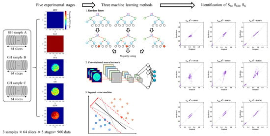
2.2. Data Acquisition and Pre-Process

The CT images from the GH experiment were modified and normalized, as shown in Figure 4. Figure 4a presents the ImageJ window, which is an open-source software, developed at the National Institutes of Health and the Laboratory for Optical and Computational Instrumentation, that provides numerous functions to edit images [27,28]. This study used ImageJ to modify and organize the given CT images for pre-processing. Figure 4b shows 64 slices of sample B in the initial water saturation stage (according to the definitions of the five stages provided in Section 2.1). Figure 4b contains a circle-shaped image surrounded by a white part, which indicates that the cylinder contains a sample. Thus, this white must be eliminated, as shown in Figure 4c, for every image slice of a sample. ImageJ recognizes the dotted lined circle areas and removes the remaining circle area (right column in Figure 4c). The organized images are placed in the “CT,” which are then subtracted by the “DRY” stage image and divided by the difference between the “SAT” and “DRY” stages, as described in Figure 4d. The far right image in Figure 4d displays the normalized CT image, which has a scale of 0–1 due to the normalization procedure. When this image has a value of 1, it is fully saturated with water, which indicates that the sample has the highest density with respect to the current experimental conditions. In contrast, a value of 0 indicates that the sample is saturated with air, which is the lowest density value at the experimental conditions.

In this study, we assume that the sample matrix is fixed in its original position, which indicates that there is only a change in the phase. The normalization procedure removes the effect of the sand sample structure, such that we can only quantitatively consider the behaviors of each phase in the porous media. Therefore, the GH CT data from different samples can be used together to model fluid behaviors because they only reflect changes in the internal fluid and not the sample frame. Figure 5 displays the raw and normalized sample images for the first slice of sample B. In Figure 5b, the “DRY” and “SAT” images have 0 and 1 value circle-shaped sample areas, respectively. Theoretically, the samples should only have values between 0 and 1 based on the normalization. However, certain samples have values less than 0 or greater than 1 due to measurement error or other physical effects from the experimental conditions. In this study, these sample values were modified to 0 or 1 for samples with values less than 0 or greater than 1, respectively.

Saturation of the three phases (i.e., gas, water, and GH) must be assigned for the given GH CT images to construct the training data, which is the labeling for the normalized GH CT images. The first two stages among the five stages theoretically have clear saturation values: S_W = 0, S_GH = 0, and S_G = 1 for the “DRY” stage and S_W = 1, S_GH = 0, and S_G = 0 for the “SAT” stage. In the other three stages, mass balance was used to compute each saturation, as listed in

Table 1. Calculations for the saturation labeling in the three experimental stages: “IWS”, “GH” and “GTW”.

Experimental Stage	SW (Density, g/cc)	SGH (Density, g/cc)	SG (Density, g/cc)
“IWS” (14.7 psi, 18 °C)	SW,IWS (1)	SGH,IWS = 0	1—SW,IWS (0.000678)
“GH” (2500 psi, 16 °C)	SW,GH = 0	SGH,GH (0.91)	1—SGH,GH (0.143)
“GTW” (2900 psi, 16 °C)	SW,GTW (1.008)	SGH,GTW = SGH,GH	1—SW,GTW—SGH,GTW (0.167)

. The normalized CT values have 1 and 0 for the maximum and minimum, respectively. The maximum and minimum normalized CT values are corresponding to 100% water (“SAT”) or 100% gas (“DRY”) saturated because water density is about 1 g/cc and gas density is almost 0 compared to that of water. Therefore, the average density should correspond to the normalized CT value as following Equation (2):

$${\mathrm{S}}_{\mathrm{W}}\times {\mathrm{d}}_{\mathrm{W}}+{\mathrm{S}}_{\mathrm{GH}}\times {\mathrm{d}}_{\mathrm{GH}}+{\mathrm{S}}_{\mathrm{G}}\times {\mathrm{d}}_{\mathrm{G}}={\mathrm{CT}}_{norm}^{avg},$$

(2)

$${\mathrm{S}}_{\mathrm{W},\mathrm{IWS}}\times 1+\left(1-{\mathrm{S}}_{\mathrm{W},\mathrm{IWS}}\right)\times 0.000678={\mathrm{CT}}_{norm}^{avg},$$

(3)

$${\mathrm{S}}_{\mathrm{GH},\mathrm{GH}}\times 0.91+\left(1-{\mathrm{S}}_{\mathrm{GH},\mathrm{GH}}\right)\times 0.143={\mathrm{CT}}_{norm}^{avg},$$

(4)

$${\mathrm{S}}_{\mathrm{W},\mathrm{GTW}}\times 1.008+\left(1-{\mathrm{S}}_{\mathrm{W},\mathrm{GTW}}-{\mathrm{S}}_{\mathrm{GH},\mathrm{GTW}}\right)\times 0.167={\mathrm{CT}}_{norm}^{avg},$$

(5)

$${\mathrm{CT}}_{norm}^{avg}=\frac{1}{n_c}{\sum }_{i=1}^{n_c}{\mathrm{CT}}_{norm, i},$$

(6)

where ${\mathrm{S}}_{\mathrm{W},\mathrm{IWS}}$ is the saturation of “water” in the “IWS” stage, the first and second subscript mean the fluid phase and experimental stage, respectively. In Equation (3), the constant value 1 and 0.000678 g/cc are the density of water and gas at the conditions in the “IWS” stage, respectively. The gas density of “IWS” and the water density of “GTW” are assumed as 0 and 1, respectively, for the satisfaction of Equation (2) in this study. In Equations (3)–(5), they all satisfy the sum of saturations equals 1 in each of the stages (Table 1). ${\mathrm{CT}}_{norm}^{avg}$ of Equation (6) is the average normalized CT values from all data points in one image slice among 64 slices, $n_c$, of the actual sample part (the circle-shaped area in Figure 5). Here, $n_c$ is 47,992 at the experimental conditions used in this study. In the “IWS”, “GH”, and “GTW” stages, we previously are aware of one of the three saturations and all the densities under certain experimental conditions (see the first column of Table 1), which allows us to calculate the saturation values of each phase. Therefore, the collected CT images can be labeled with saturation values based on the given conditions and Equations (2)–(5). The GH saturation of the “GTW” stage should be identical to that of the “GH” stage, assuming that the same generated GH also exists in the “GTW” The labeling was conducted for each slice such that one slice was paired with three saturation values: S_GH, S_W, and S_G.

2.3. Machine Learning Methodologies

2.3.1. Random Forest

The random forest (RF) has been used as one of the powerful machine learning methods in numerous previous studies to address prediction problems for a target parameter based on given data. The RF consists of multiple decision trees, where each decision tree is constructed, as shown in Figure 6. Figure 6a provides n sample data with a d property. The property d is the explanatory variable, which is one pixel point of the normalized CT image slice in this study. The saturation of each phase is the dependent variable, which is represented by m₁ and m₂ in Figure 6a. For example, in Figure 6a, those empty and filled circles (m₁ and m₂) are one of water, GH, or gas saturation values of the training samples and they are arrayed in descending order of an assigned property. As described in the four columns of Figure 6a, the training data is organized in descending order according to a specific property from the first property to the last. The RF finds the decision boundary to obtain the minimum sum of two MSVs (mean square variance) from two divided groups. There are d minimum MSVs from each d property and the final decision boundary is selected according to the overall minimum MSV. In case of this study, the minimum MSV will be selected considering for the all three phase saturations. The fixed decision boundary separates the training data into two groups, as described in Figure 6b. These procedures are repeated to partition the given training data until it reaches a maximum depth in the decision tree. More data partitioning results in improved data separation performance until a certain level. However, data partitioning may also cause poorer data separation after immoderately excessive partitioning, which is known as the overfitting problem. This is followed by pruning to prevent or mitigate overfitting.

Figure 7 illustrates the principle of prediction by the RF based on multiple decision trees. Figure 7a shows an entire given training data pool. Different types of decision trees are trained from different k datasets, which are generated via bootstrapping (Figure 7b). The number of decision trees is k, corresponding to the selected k datasets. Each decision tree separately yields its own prediction results, which is known as bootstrap aggregation (Figure 7c). Each result is summarized for majority voting, such that we can obtain the final results (Figure 7d,e). Multiple decision trees can lead to the stochastically stable prediction of the target parameter. Thus, a larger number of decision trees yields improved RF stability and performance in most cases. Despite this, a proper number of decision trees must be selected due to the computational cost required to train a number of decision trees.

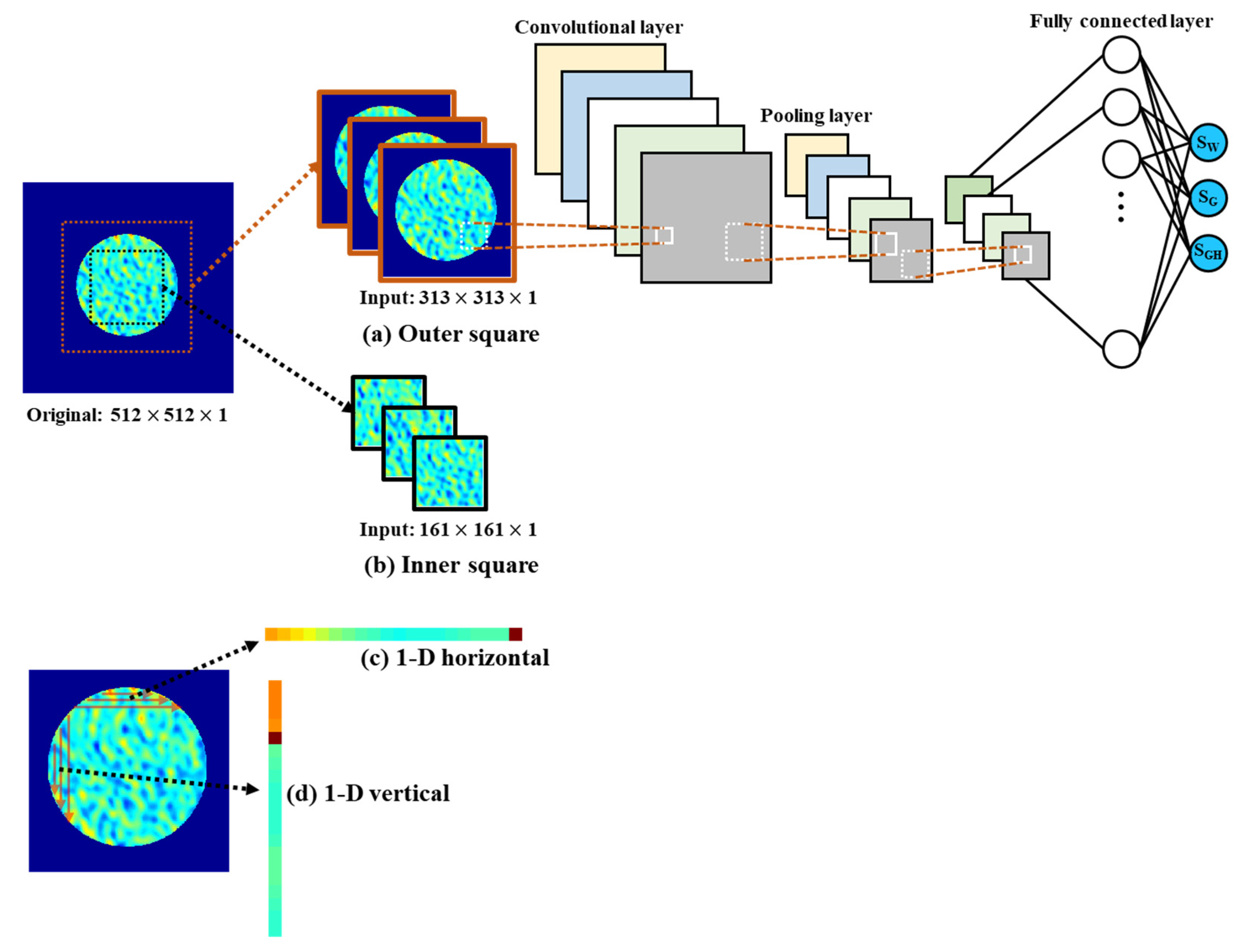
2.3.2. Convolutional Neural Network

The convolutional neural network (CNN) is one of the neural network methodologies, which manages images without pre-processing, such as flattening, and extracts features from images via convolution or subsampling [29,30]. CNN has been used in a variety of fields to obtain insight and the proper solution from large amounts of image data, e.g., handwritten recognition, human action recognition, and image classification [30,31,32,33].

Figure 8 shows a schematic image of the CNN applied to the GH CT images in this study. Input images are exposed to convolution and pooling procedures for feature extraction. Then, it ends with a fully-connected layer, where the final three nodes must be the three saturation values of each phase. The training performance of the CNN highly depends on hyper-parameters, such as the number or size of the convolutional and pooling layers. This study used AutoKeras, which efficiently and automatically searches for a proper neural architecture [34]. However, we also note that the structure of the input data can highly affect the performance of the CNN performance. Figure 8a–d displays the different types of input data structure, which we tested to find obtain the suitable input format for the GH CT images.

2.3.3. Support Vector Machine

The support vector machine (SVM), which is one of the supervised machine learning algorithms, was proposed by Vapnik and Chervonekis in 1963. If we assume that a set of data in 2-D space consist of two classes, this dataset can be classified by several hyperplanes (Figure 9). The SVM determines a maximum-margin hyperplane to distinguish each group and the data on the margin are referred to as support vectors (Figure 9). Two additional techniques have been used with the SVM to solve more complex problems: soft margin and kernel trick. When there are difficulties associated with classifying the data using an exact hyperplane, the concept of the soft margin can be introduced into the SVM [35]. The kernel trick enables nonlinear classification by converting a problem that is not linearly classified in a given dimension into a high-dimensional feature space [36].

The SVM can also handle a regression problem, as shown in Vapnik et al. [37]. In the application of a regression problem, the SVM attempts to fit the optimized hyperplane with as many data as possible within the epsilon, which is a reverse optimization compared with the classification problem. Support vector regression uses a slack variable that plays a role similar to the soft margin in the classification problem [38].

3. Results

These three machine learning methods were applied to the training data from the three datasets: samples A, B, and C. The GH CT images of each GH sample were broken into 96 slices and the first 64 slices were used for the five experiment stages to construct the training data. Therefore, 3 GH samples $\times$ 64 slices $\times$ 5 stages is equal to 960 samples, which consist of the training data for machine learning. Figure 10 shows the normalized CT values for the first slice of sample A, which are represented in the histogram. Figure 10b,c displays the histogram of the normalized CT values for the circled and outer areas in the images, respectively, marked with the yellow dotted line. The overall normalized CT values increase from the “IWS” to “GTW” stages based on the changes in the stage.

Table 2. Conditions and settings for the training of the RF, CNN, and SVM.

Method	List	Condition
Common condition	Training data	864
	Test data	96 (10% of the entire data)
RF	Maximum depth	10
	Number of trees	200
	Number of properties	219
	Data size of one sample	47,996
CNN	Validation data	96 (10% of the whole data)
	Maximum trials	50
	Data size of one sample	313 by 313 (Figure 8a) 161 by 161 (Figure 8b) 47,996 by 1 (Figure 8c) 47,996 by 1 (Figure 8d)
SVM	Kernel function	Linear
	Data pre-process	Standardize
	Data size of one sample	47,996

lists the other detailed training information for the three methodologies. The size of one data sample depends on the machine learning method and the structure of the input data. The number of properties for bootstrap of RF (Figure 7b) is the square root of the number of data points in one sample. Training and test data are applied to each machine learning technique. For the CNN, the validation data is a part of the training data and the result of the validation is presented together with the training data.

The RF and CNN were realized in the Python language environment using a workstation whose specifications are as follows: Intel Xeon Gold 6136 central processing unit with 3 and 2.99 GHz processors and 128 GB random-access memory. The SVM was conducted in MATLAB using the same workstation. The methods required approximately 28, 31, and 1 min for the RF, CNN, and SVM, respectively. Although the computation time for each machine learning methodology depends on its hyper-parameters, we speculated that the RF and SVM would require less time as compared with the CNN, which specifically has many parameters that must be fixed due to a comparatively complicated CNN structure. Thus, the RF and SVM are more advantageous with respect to the computational cost as compared with the CNN.

3.1. RF Results

Figure 11 shows the training and test results for the RF. The X and Y axis represent the original data and the values predicted by the RF, respectively. Thus, more data positioned on the 1:1 indicates a better matching performance. The number of scattered purple points is 864. The more points in the same position results in a darker color, indicating overlap. As shown in Figure 11a, most data points are positioned on the 1:1 line. Their correlation coefficient R² values are larger than 0.99, which indicates that the original and predicted values are significantly related and fitted to each other. In Figure 11a, the gas saturation, in particular, shows a strong correlated trend (R² = 0.99976), as compared with the S_W and S_GH. This is because the density of gas is significantly less than that of water or the GH, which allows us to more easily distinguish the gas phase from the two other phases.

Certain original data have zero values for S_W and S_GH in the first and second pictures of Figure 11a,b. The original S_G values at or near zero were sufficiently predicted in both the training and test data. In contrast, the S_W and S_GH values near zero exhibit overestimation in the bottom-left corner of the first and second pictures in Figure 11a,b. Overall, the RF yields a significantly decent performance for both the training and test results.

3.2. CNN Results

Figure 12, Figure 13, Figure 14 and Figure 15 present the training results from the CNN with different types of input data structures (Figure 8a–d). The structure of the input data is a 2-D square-shape in both Figure 12 and Figure 13, where the R² values are less than 0.5, which are considerably low compared with the results of the RF in Figure 11. We observe no specific diagonal trends in the scattered data in all the images of Figure 12 and Figure 13. In contrast, Figure 14 and Figure 15 exhibit a diagonally scattered trend, as compared with Figure 12 and Figure 13. The R² values of the CNN results with the 1-D input data are larger than 0.9 for every result (Figure 14 and Figure 15). We note that the overall results are similar between Figure 14 and Figure 15 with respect to the trend of the scattered points and R² values, which indicates that the direction of the 1-D data does not lead to a substantial difference in this study.

As previous studies have shown, the CNN should excel at feature extraction from specific trends or patterns in images [39,40]. Thus, we expect the CNN to function correctly for image-oriented performance. However, the CNN does not function in this manner, considering that Figure 14 and Figure 15 depict an improved performance over Figure 12 and Figure 13. The former two results derive from 2-D images of the CT images, which should reflect certain 2-D characteristics from the input data (Figure 12 and Figure 13). In contrast, the latter two results of the CNN with 1-D input data should only consider the relationship of neighborhood grids. Overall, considering the relationship between each CT value for one grid and the saturation values is difficult because one entire slice has only three saturation values (S_W, S_GH, and S_G), which correspond to averaged normalized CT values based on the labeling. In particular, the outer squared 2-D input image (Figure 8a) resulted in a low correlation and poor matching performance because it has an unnecessary component, i.e., out of one sand sample, in the input data image, whose scale is between 0 and 1, which may have caused a loss of meaning and sensitivity with respect to the normalized CT values. In contrast, the inner squared 2-D input image (Figure 8b) showed improvement compared with the outer squared 2-D input case due to the elimination of the unnecessary component, such that its scale became narrower than between 0 and 1 (see Figure 10b,c). This appears to be helpful for the enhancement of the performance by reserving meaningful variations from the data.

3.3. SVM Results

The SVM yielded outstanding performance for the training results, which showed R² values larger than 0.9. We note that the SVM mitigated the overestimation of near zero values in the original S_W and S_GH, as compared with both the RF and CNN (bottom left corner of Figure 16a). Despite the decent performance by the SVM, the test results were not reliable, especially for the S_W and S_GH (the first and second images in Figure 16b). The test results for gas saturation show an overall well-matching performance between the original and predicted data, which is because the gas saturation should have discriminating features compared with the S_W and S_GH in terms of their typical normalized CT values. Despite sufficient potential as a candidate among the other machine learning methods, the SVM requires validation for test performance in future studies.

Table 3. MSE results of the training and test datasets using the RF, CNN, and SVM.

Method	Input Data	MSE (×10−4): SW, SGH, SG				Average (×10−4)
RF	Sample part (47,996 grid, Figure 10b)	Training	7	7	3	6
		Test	39	40	2	27
CNN	2-D outer square (313 by 313, Figure 8a)	Training	1117	550	1176	948
		Test	1388	1055	1752	1398
	2-D inner square (161 by 161, Figure 8b)	Training	857	513	850	740
		Test	2722	963	4990	2892
	1-D horizontal (47,996, Figure 8c)	Training	38	37	23	33
		Test	38	42	18	33
	1-D vertical (47,996, Figure 8d)	Training	39	36	25	33
		Test	36	39	19	31
SVM	Sample part (47,996 grid, Figure 10b)	Training	11	14	5	10
		Test	652	645	4	434

lists the MSE results of the RF, CNN, and SVM for the training and test datasets. The MSE is calculated as follows for the training and test datasets, respectively:

$$MS{E}_{train}=\frac{1}{n_{train}}{\sum }_{i=1}^{n_{train}}{\left(Ori{g}_{i, train}-Pre{d}_{i, train}\right)}^2,$$

(7)

$$MS{E}_{test}=\frac{1}{n_{test}}{\sum }_{i=1}^{n_{test}}{\left(Ori{g}_{i, test}-Pre{d}_{i, test}\right)}^2,$$

(8)

where $n_{train}$ and $n_{test}$ are the number of training and test datasets, respectively, $Ori{g}_i$ is the original ith data, and $Pre{d}_i$ represents the predicted data for the ith original data.

As shown in Figure 11, Figure 12, Figure 13, Figure 14, Figure 15 and Figure 16, the RF exhibited the best performance in terms of the smallest MSE results in both the training and test datasets, i.e., 6 $\times$ 10⁻⁴ and 27 $\times$ 10⁻⁴, respectively. Results from the 2-D input image for the CNN had the largest MSE, which is approximately 100-fold higher than the other results. The SVM yielded low MSE results for the training dataset. However, the average MSE from the test dataset was larger. If the MSE of the training data for the SVM was quantitatively similar to the RF, we would be able to be propose it as a reliable cost-effective machine learning method appropriate for saturation modeling of the GH CT images.

4. Discussion

Based on our results, the RF yielded the best prediction performance for both the training and test datasets compared with the CNN and SVM. The RF is advantageous because it is reliable even with limited data, especially compared to the CNN, as the RF defines each decision tree with several parameters, such as the decision boundary, whose value is, at most, several decades or hundreds of parameters. In addition, RF has robustness even with a restricted number of training data or wide variability of data because RF works to figure out how input data properties distinguishably separate output data, important function to identify data patterns [41]. Although the SVM exhibited sufficient performance for the training dataset, the results for the test dataset were not as good as that of the training dataset. This is due to one or both of the two following reasons: lack of training data or a highly non-linear relationship between the explanatory parameters and target parameter. A lack of data will lead to poor learning while high non-linearity causes difficulties with respect to learning in any type of learning algorithm. The CNN requires a substantial amount of training data to find its numerous parameters, such as the weight and bias values in the neural network, which number in the thousands, or more. Additionally, the output data for training corresponds to the average normalized CT values in this study, such that it is difficult for the CNN to understand the features of a given CT image. This is an internal problem due to the structure of the training data, rather than a drawback of the CNN. Therefore, the CNN should yield improved performance with extra training data or a more appropriate training data structure.

5. Conclusions

This paper examined the applications of machine learning to X-ray CT images, especially for saturation analyses of GH resources. This study was conducted to overcome the time delay and precision limitations of existing saturation test equipment, as well as to improve the manual analysis of individual CT images. We developed machine learning models that automatically analyze the saturation of three phases by securing ~1000 CT images and data labeling via experiments.

As a result of applying the three machine learning algorithms (i.e., the RF, CNN, and SVM) to the same data, the predictive performance of the RF showed a correlation coefficient of over 95% for both the training and test datasets. In comparison, the SVM did not guarantee the predictive performance of the test dataset due to overfitting. In particular, the prediction performance of the S_GH was deteriorated in the test dataset. For the CNN, there was a limit to the application of the 2-D CNN as the CT image is a circular image. However, only the 1-D CNN showed significantly improved results. Although the CNN had a similar level of correlation as the RF, the latter exhibited improved precision in terms of the average error.

Based on the results obtained in this study, we confirm that the RF algorithm shows excellent performance for CT images, and, in particular, we identified the appropriate pre-processing methods for the input data when using the CNNs. In future studies, the proposed method will be helpful as a first step to identify all three phases in the process of GH dissociation. In addition, the augmentation technique, which increases the amount of data to 1000 levels, used in this study should be applicable. This, however, requires the ability to secure additional experimental data.

In this study, the proposed pre-processing such as the normalization of CT images is already designed to be applicable to another target of GH core or reservoir because the normalization removes pore structure effect in CT images. Therefore, the proposed saturation identification method would be workable regardless of GH formation types such as pore-filling or grain-coating [18,42]. In spite of that, we will keep considering any potential possibility causing different characteristics from another GH target for GH saturation modeling and try to thoroughly validate the universality of the proposed method.

References

1. Burdine, N.T. Relative permeability calculations from pore size distribution data. Soc. Pet. Eng. 1953. [Google Scholar] [CrossRef]
2. Beard, D.C.; Weyl, P.K. Influence of texture on porosity and permeability of unconsolidated sand. AAPG Bull. 1973, 57, 349–369. [Google Scholar] [CrossRef]
3. Katz, A.J.; Thompson, A.H. Quantitative prediction of permeability in porous rock. Phys. Rev. B 1986, 34. [Google Scholar] [CrossRef] [PubMed]
4. Akin, S.; Kovscek, A.R. Computed tomography in petroleum engineering research. Geol. Soc. Lond. 2003, 215, 23–38. [Google Scholar] [CrossRef]
5. Sondergeld, C.H.; Newsham, K.E.; Comisky, J.T.; Rice, M.C.; Rai, C.S. Petrophysical considerations in evaluating and producing shale gas resources. Soc. Pet. Eng. 2010. [Google Scholar] [CrossRef]
6. KIGAM. Studies on Gas Hydrate Development and Production Technology; Report GP2012-02502014(3); Pacific Northwest National Laboratory: Daejeon, Korea, 2014; p. 330.
7. Lee, M.; Suk, H.; Lee, J.; Lee, J. Quantitative Analysis for Gas Hydrate Production by Depressurization Using X-ray CT. In Proceedings of the 2018 Joint International Conference of the Geological Science & Technology of Korea, KSEEG, Busan, Korea, 17–20 April 2018; p. 363. [Google Scholar]
8. Suk, H.; Ahn, T.; Lee, J.; Lee, M.; Lee, J. Development of gas hydrate experimental production system combined with X-ray CT. J. Korean Soc. Miner. Energy Resour. Eng. 2018, 55, 226–237. [Google Scholar] [CrossRef]
9. KIGAM. Field Applicability Study of Gas Hydrate Production Technique in the Ulleung Basin; Report GP2016-027-2016(1); Pacific Northwest National Laboratory: Daejeon, Korea, 2016; pp. 37–73.
10. KIGAM. Gas Hydrate Exploration and Production Study; Report GP2016-027-2017(2); Pacific Northwest National Laboratory: Daejeon, Korea, 2017; pp. 164–199.
11. Wang, J.; Zhao, J.; Yang, M.; Li, Y.; Liu, W.; Song, Y. Permeability of laboratory-formed porous media containing methane hydrate: Observations using X-ray computed tomography and simulations with pore network models. Fuel 2015, 170–179. [Google Scholar] [CrossRef]
12. Mikami, J.; Masuda, Y.; Uchida, T.; Satoh, T.; Takeda, H. Dissociation of natural gas hydrate observed by X-ray CT scanner. Ann. N. Y. Acad. Sci. 2006, 912. [Google Scholar] [CrossRef]
13. Kneafsey, T.J.; Tomutsa, L.; Moridis, G.; Seol, Y.; Freifeld, B.; Taylor, C.; Gupta, A. Methane hydrate formation and dissociation in a partially saturated core-scale sand sample. J. Pet. Sci. Eng. 2007, 56, 108–126. [Google Scholar] [CrossRef] [Green Version]
14. Holland, M.; Schultheiss, P.; Roberts, J.; Druce, M. Observed Gas Hydrate Morphologies in Marine Sediments. In Proceedings of the 6th International Conference on Gas Hydrate (ICGH 2008), Vancouver, BC, Canada, 6–10 July 2008. [Google Scholar] [CrossRef]
15. Liu, Y.; Song, Y.; Chen, Y.; Yao, L.; Li, Q. The detection of tetrahydrofuran hydrate formation and saturation using magnetic resonance imaging technique. J. Nat. Gas Chem. 2010, 19, 224–228. [Google Scholar] [CrossRef]
16. Seol, Y.; Kneafsey, T.J. Methane hydrate induced permeability modification for multiphase flow in unsaturated porous media. J. Geophys. Res. 2011, 116, B08102. [Google Scholar] [CrossRef]
17. Wu, N.; Liu, C.; Hao, X. Experimental simulations and methods for natural gas hydrate analysis in China. China Geol. 2018, 1, 61–71. [Google Scholar] [CrossRef]
18. Lei, L.; Seol, Y.; Choi, J.; Kneafsey, T. Pore habit of methane hydrate and its evolution in sediment matrix—Laboratory visualization with phase-contrast micro-CT. Mar. Pet. Geol. 2019, 104, 451–467. [Google Scholar] [CrossRef] [Green Version]
19. Kim, S.; Kim, K.H.; Min, B.; Lim, J.; Lee, K. Generation of synthetic density log data using deep learning algorithm at the Golden field in Alberta, Canada. Geofluids 2020, 2020, 5387183. [Google Scholar] [CrossRef] [Green Version]
20. Lee, K.; Lim, J.; Yoon, D.; Jung, H. Prediction of shale gas production at Duvernay Formation using deep-learning algorithm. SPE J. 2019, 24, 2423–2437. [Google Scholar] [CrossRef]
21. Waldeland, A.; Jensen, A.C.; Gelius, L.-J.; Solberg, A.H.S. Convolutional neural networks for automated seismic interpretation. Lead. Edge 2018, 37, 529–537. [Google Scholar] [CrossRef]
22. Huang, L.; Dong, X.; Clee, E.A. Scalable deep learning platform for identifying geologic features from seismic attributes. Lead. Edge 2017, 36, 249–256. [Google Scholar] [CrossRef]
23. Chen, Z.; Liu, X.; Yang, J.; Littile, E.; Zhou, Y. Deep learning-based method for SEM image segmentation in mineral characterization, an example from Duvernay Shale samples in Western Canada Sedimentary Basin. Comput. Geosci. 2020, 138, 104450. [Google Scholar] [CrossRef]
24. Chauhan, S.; Rühaak, W.; Anbergen, H.; Kabdenov, A.; Freise, M.; Wille, T.; Sass, I. Phase segmentation of X-ray computer tomography rock images using machine learning techniques: An accuracy and performance study. Solid Earth 2016, 7, 1125–1139. [Google Scholar] [CrossRef] [Green Version]
25. Karimpouli, S.; Tahmasebi, P. Segmentation of digital rock images using deep convolutional autoencoder networks. Comput. Geosci. 2019, 126, 142–150. [Google Scholar] [CrossRef]
26. Krevor, S.; Pini, R.; Zuo, L.; Benson, S. Relative permeability and trapping of CO2 and water in sandstone rocks at reservoir conditions. Water Resour. Res. 2012, 48, W02532. [Google Scholar] [CrossRef]
27. Abramoff, M.D.; Magalhães, P.J.; Ram, S.J. Image processing with ImageJ. Biophotonics Int. 2004, 11, 36–42. [Google Scholar]
28. Schneider, C.A.; Rasband, W.S.; Eliceiri, K.W. NIH image to ImageJ: 25 years of image analysis. Nat. Methods 2012, 9, 671–675. [Google Scholar]
29. LeCun, Y.; Bengio, Y. Convolutional networks for images, speech, and time-series. Handb. Brain Theory Neural Netw. 1995, 3361, 1995. [Google Scholar]
30. LeCun, Y.; Haffner, P.; Bottou, L.; Bengio, Y. Object Recognition with Gradient-Based Learning. In Shape, Contour and Grouping in Computer Vision; Springer: Berlin/Heidelberg, Germany, 1999; Volume 1681. [Google Scholar]
31. Ji, S.; Xu, W.; Yang, M.; Yu, K. 3D convolutional neural networks for human action recognition. IEEE Trans. Pattern Anal. Mach. Intell. 2012, 35, 221–231. [Google Scholar]
32. Lin, B.; Wei, X.; Junjie, Z. Automatic recognition and classification of multi-channel microseismic waveform based on DCNN and SVM. Comput. Geosci. 2019, 123, 111–120. [Google Scholar]
33. Krizhevsky, A.; Sutskever, I.; Hinton, G.E. ImageNet classification with deep convolutional neural networks. Commun. ACM 2017, 60. [Google Scholar] [CrossRef]
34. Jin, H.; Song, Q.; Hu, X. Auto-keras: Efficient neural architecture search with network morphism. arXiv 2018, arXiv:1806.10282v2. [Google Scholar]
35. Cortes, C.; Vapnik, V.N. Support-vector networks. Mach. Learn. 1995, 20, 273–297. [Google Scholar] [CrossRef]
36. Boser, B.E.; Guyon, I.M.; Vapnik, V.N. A Training Algorithm for Optimal Margin Classifiers. In Proceedings of the Fifth Annual Workshop on Computational Learning Theory—COLT ‘92, Pittsburgh, PA, USA, 27–29 July 1992; p. 144. [Google Scholar] [CrossRef]
37. Vapnik, V.; Golowich, S.E.; Smola, A.J. Support Vector Method for Function Approximation, Regression Estimation and Signal Processing. In Proceedings of the Advances in Neural Information Processing Systems 9, Denver, CO, USA, 2–5 December 1996; Moser, M.C., Jordan, M.I., Petsche, T., Eds.; MIT Press: Cambridge, MA, USA, 1997; pp. 281–287. [Google Scholar]
38. Drucker, H.; Burges, C.C.; Kaufman, L.; Smola, A.J.; Vapnik, V.N. Support Vector Regression Machines. In Proceedings of the Advances in Neural Information Processing Systems 9, Denver, CO, USA, 2–5 December 1996; Moser, M.C., Jordan, M.I., Petsche, T., Eds.; MIT Press: Cambridge, MA, USA, 1997; pp. 155–161. [Google Scholar]
39. LeCun, Y.; Bengio, Y.; Hinton, G. Deep learning. Nature 2015, 521, 436–444. [Google Scholar]
40. Chu, M.; Min, B.; Kwon, S.; Park, G.; Kim, S.; Huy, N.X. Determination of an infill well placement using a data-driven multi-modal convolutional neural network. J. Pet. Sci. Eng. 2019, 106805. [Google Scholar] [CrossRef]
41. Ramos, G.A.R.; Akanji, L. Data analysis and neuro-fuzzy technique for EOR screening: Application in Angolan oilfields. Energies 2017, 10, 837. [Google Scholar] [CrossRef]
42. Chen, X.; Espinoza, D.N.; Luo, J.S.; Tisato, N.; Flemings, P.B. Pore-scale evidence of ion exclusion during methane hydrate growth and evolution of hydrate pore-habit in sandy sediments. Mar. Pet. Geol. 2020, 117, 104340. [Google Scholar] [CrossRef]
Figure 1. A schematic diagram of the GH visualization system at KIGAM [6,8].
Energies 13 05032 g001
Figure 2. The installed X-ray CT equipment for the GH visualization system at KIGAM [8,10].
Energies 13 05032 g002
Figure 3. Flow chart of the GH formation experiment and CT scanning to obtain the training data for machine learning. (a) the first stage of the experiments to construct a sand sample; (b) the second stage to make a sample fully saturated with water; (c) the third stage with initial water and gas saturation; (d) the fourth stage to form gas hydrate by pressurization; (e) the fifth stage with only water and gas hydrate after replacement of gas by water.
Energies 13 05032 g003
Figure 4. Modification and normalization of the CT images using ImageJ. (a) the window of ImageJ software; (b) scanned raw core images of one sample from GH experiments; (c) removal of useless part from raw images; (d) normalization of images with those of “DRY” and “SAT” stages.
Energies 13 05032 g004
Figure 5. Examples of CT images for the first slice in sample B. (a) raw CT images of the five experimental stages; (b) normalized CT images for the five stages.
Energies 13 05032 g005
Figure 6. The construction of a decision tree with recursive partitioning and pruning based on n sample data of the d property. (a) finding the best decision boundary having the largest purity of data; (b) making branches according to proper decision boundaries; (c) removal of excessive branches to prevent overfitting.
Energies 13 05032 g006
Figure 7. A random forest (RF) with multiple decision trees for the prediction of the target parameters.
Energies 13 05032 g007
Figure 8. A schematic diagram of the CNN application with different input data in the CT image. (a) the first option to construct input data and it is the largest amount of data compared to the rest of three options; (b) the second option to construct input data with only inner area from the outer square; (c) the third option for input data in one dimension and it attaches pixels in horizontal direction; (d) the fourth option for input data constructed in vertical direction.
Energies 13 05032 g008
Figure 9. A conceptual description of SVM classification.
Energies 13 05032 g009
Figure 10. The normalized CT values in the first slice of sample A presented with a color scale.
Energies 13 05032 g010
Figure 11. (a) Training and (b) test results from the RF.
Energies 13 05032 g011
Figure 12. The training (a) and test (b) results from the CNN with the outer squared input data (Figure 8a).
Energies 13 05032 g012
Figure 13. The training (a) and test (b) results from the CNN with the inner squared input data (Figure 8b).
Energies 13 05032 g013
Figure 14. The training (a) and test (b) results from the CNN with the 1-D horizontal input data (Figure 8c).
Energies 13 05032 g014
Figure 15. The training (a) and test (b) results from the CNN with the 1-D vertical input data (Figure 8d).
Energies 13 05032 g015
Figure 16. The training (a) and tests (b) results from the SVM.
Energies 13 05032 g016