Abstract
This paper presents a multi-terminal traveling-wave-based fault location method for phase-to-ground fault in non-effectively earthed distribution systems. To improve the accuracy of fault location, a two-terminal approach is used to identify the faulty branch and a single-ended approach is followed to determine the fault distance based on the arrival time of reflected traveling waves. Wavelet decomposition is employed to extract the time-frequency component of the aerial-mode traveling waves. Magnitude and polarity of the wavelet coefficients are used to estimate the fault distance starting from the propagation fault point to the branch terminal. In addition, the network is divided into several sub-networks in order to reduce the number of measurement units. The effectiveness of this approach is demonstrated by simulations considering the phase-to-ground fault that happens at different positions in the distribution network.
1. Introduction
Non-grounded systems and arc-suppression-coil-grounded systems are widely used in distribution networks in China. They are generally called non-effectively grounded systems, where phase-to-ground fault location becomes difficult due to the weak fault feature. To solve this problem, various approaches have been proposed, including impedance-based methods [1,2,3,4,5,6,7,8,9], traveling wave-based methods [10,11,12,13,14,15,16,17,18,19,20,21,22,23], and artificial intelligence-based methods [24,25,26].
Impedance-based methods use voltage and current of the mains frequency to estimate fault distance. The potential assumption is that the fault current is large enough to be distinguished from the load current [1,2,3,4,5,6,7,8]. As is well known, however, in a non-effectively grounded system, fault current aggregates the capacitive currents of each feeder, which is weak and is not easy to be used for fault location [9].
Traveling-wave (TW)-based fault location, which is nearly unaffected by the fault current strength of the mains frequency, shows its superiority in the non-effectively grounded systems [10,11,12,13,14,15,16,17,18,19,20,21,22,23]. According to the number of measurement units used, TW-based approaches can be divided into single-ended schemes [10,11,12,13,14,15] and multi-terminal schemes [16,17,18,19,20,21,22,23].
The single-ended method uses the features extracted from the incident and reflected TWs to estimate the fault location. In [10], the fundamental frequency spectrum component and the first subordinate component of the ground mode voltage are used to match a relationship between the fault distance and the dominant frequency component. Therefore, a database has to be developed in advance to describe this relation in the condition of different network topologies. In addition, the ground mode wave is not stable in practice due to the fact that the velocity may change severely when the wave undergoes different transmission mediums. Literature [11] decomposes the fault-originated TW through continuous wavelet transform, which is a sort of time-frequency decomposition. The characteristic frequency of the decomposed component is related to the TW propagation paths throughout the network. In this way, the fault location is refined correspondingly. The method used in [11] is further improved with an integrated time-domain information in [12]. Literature [13] presents a new method based on the electromagnetic time-reversal (EMTR) theory to locate faults in power networks. The employed single-ended measurement device adopts a sampling frequency as 1 G samples/s. In [14], the transient voltage of the transmission line is analyzed through wavelet transform, and the characteristic frequencies of the converted signal are obtained. The fault location is determined according to the correlation between these characteristic frequencies and some specific paths. Only one measurement unit with the sampling rate of 1 MHz is needed, however, the average absolute error is large. A single-ended reclosure-generating TW-based fault location scheme is proposed in [15], where the time difference between the reclosing instant and the arrival time of TW reflected from the fault point is employed to estimate the fault distance. This method is not available in the network without the reclosure operation. In single-ended schemes, how to get sufficient fault information with a single terminal is the key point and it is important to take advantage of the reflected TWs to cope with the multi-branch effect. Thus, the effective features of TW reflection at different positions (e.g., line junctions and line terminals) are expected.
Multi-terminal methods are able to deal with fake estimations caused by possible fault points at equal electrical distance from the measurement unit [16,17,18,19,20,21,22,23]. However, the number of measurement units is proportional to the complexity of the network and is inversely proportional to the amount of TW reflections involved. In [16,17], two-terminal fault location is applied in a transmission system. Both measurement units are synchronized using the global positioning system (GPS). Sparsely distributed measurement units with GPS are deployed in a distribution network to sample the transient voltage wave for fault location [18]. Since the velocity of such voltage wave is not stable for a phase-to-ground fault, the accuracy of the fault location is reduced. In [19], the measurement unit is installed at each branch terminal in a multi-branch network in order to improve the locating performance. However, more measurement units mean higher cost and complicated maintenance. A mathematical morphology-based filter is used in [20] to detect the arrival time of travelling waves from fault-originated transient signals. Only the measurement units on the main line ends are required. However, this scheme is not available for a multi-level branch network, which is widely used in real distribution networks. In [21], time difference of TW arrival is used to determine the faulted branch, where the fault distance is derived from a relationship between the peak of energy spectrum and the electrical length at possible fault points. This relationship depends on a great number of offline simulations. In [22], TW’s reflection and refraction at line junctions are investigated in time domain and S-domain. The proposed fault location method considers the effect of TW arrival time delay caused by transformers. The time-stamping is determined by the capture of fault-originated TW through multiple measurement units with GPS time synchronization and radio communication. In [23], variational mode decomposition and teager energy operator (VMD-TEO) are used, and a few measurement units have to be installed at both ends of the main line and terminals of the branch that has sub-branches. Multi-terminal approaches mitigate the fake fault estimation and improve the locating accuracy. Nevertheless, the increased number of measurement units causes higher cost and maintenance.
Regardless of the specific methodology, one of the challenges is to detect prominent features from the incident and reflected TWs, which are usually very weak in phase-to-ground faults. Fortunately, the strength of the initial TW and the polarity of TW reflection at line ends are salient. Therefore, in this paper, a two-step fault location approach considering the above-mentioned features is presented. By using wavelet decomposition of the aerial-mode TW, fault location can be determined either on the main line or on the faulted branch through time difference of the TW heads measured synchronously at both ends of the main line, which follows the traditional two-terminal method. Then, amplitude and polarity of the wavelet coefficients obtained from the reflected TWs are taken into account to identify the reflection path and estimate the fault distance by using a single-ended approach. In order to apply the proposed method in a complex network and reduce the number of measurement units, a distribution network is divided into several sub-networks, each of which has two synchronous measurement units.
The paper is organized as follows. Section 2 describes the TW propagation properties, especially the amplitude and polarity of wavelet transformed coefficients of the incident and reflected TWs. Section 3 details the two-step fault location scheme. In Section 4, simulation results and discussions are provided, considering a real non-effectively earthed distribution system. Finally, conclusions are given in Section 5.
2. Travelling Wave Propagation Characteristics
2.1. Definition of TW Propagation Paths
According to the superposition principle, a voltage source is assumed at the fault point when a fault occurs. The fault-originated traveling wave propagates in both directions along the line and it will be reflected at branch terminals, tee points, and the fault point. Typical TW propagation paths are illustrated in Figure 1.
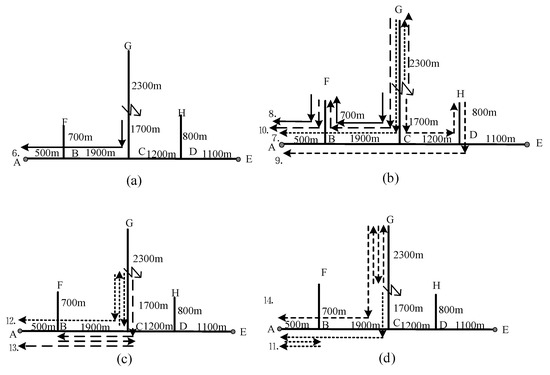
Figure 1.
Traveling wave propagation. (a) Initial Wave. (b) Branch Terminal Reflected Waves. (c) Tee Point and Fault Point Reflected Waves. (d) Hybrid Reflected Waves.
In Figure 1, B, C, and D represent tee points, and F, G, H, E represent branch terminals. One measurement unit is deployed at point A, which represents a substation. For a phase-to-ground fault on branch CG, TW undergoes different paths from the fault point to point A through line of sight and multiple reflections as described in Table 1. Regarding these propagations, four types of TW are categorized.

Table 1.
TW Propagation Paths.
- (1)
- Initial wave (IW) propagates directly from the fault point to the measurement point, which is path ① as shown in Figure 1a.
- (2)
- Branch terminal reflected waves (BTRW) reflect just once at each branch terminals, such as path ②–⑤ shown in Figure 1b. For example, path ② is represented by the dotted line. The TW starts from the fault point and goes toward the terminal of branch CG, then reflects from terminal G. Then, it goes to the tee point and turns to the direction toward point A. Similarly, the TW reflects at terminal F of branch BF, terminal H of branch DH, and both terminal G of branch CG and terminal F of branch BF, along path ③, path ④, and path ⑤, respectively.
- (3)
- Tee point or fault point reflected waves (TPRW) reflect between the “discontinuity” points except the branch terminal, e.g., path ⑦ and path ⑧ shown in Figure 1c. For example, along path ⑦, the TW reflects several times at the fault point and tee point C, but never goes to the terminal of any branches.
- (4)
- Hybrid reflected waves (HRW) undergo multiple reflections at branch terminals, tee points, and the fault point, e.g., path ⑥ and path ⑨ in Figure 1d.
2.2. Modulus-Extremum of Wavelet-Transformed Coefficients
Since the traveling wave velocity is stable on the lines, aerial-mode voltage is taken into account through Karrenbauer transformation which turns phase component into modulus. Besides, in order to identify the TW propagation paths, wavelet-transform modulus-extremum (WTME) is used to detect the arrival time, polarity, and magnitude of the incident and reflected TWs. At different reflection positions, the reflection coefficients are specified as the following [11].
Branch terminal where a step-down or a step-up power transformer is connected can be considered as an open circuit, and the corresponding reflection coefficient is close to +1;
Tee point is a junction where more than two line sections are attached. Reflection at the tee point is characterized by a negative reflection coefficient which drops into the range of −1 to 0;
The reflection coefficient at the fault point is close to −1, as the fault impedance is much smaller than the line surge impedance.
Following the conclusion obtained in [11], the polarity of WTME is summarized in (1) for different TWs.
where Pi represents the polarity and its subscript i denotes the categorized TWs. In particular, HRWodd and HRWeven indicate an odd number of reflections and an even number of reflections at the tee points, respectively.
In addition, the amplitude of WTME for different TWs is given in (2) [11].
where A represents the amplitude and its subscript stands for the type of TWs.
Without loss of generality, only the positive WTME, which is called wavelet-transform modulus-maxima (WTMM), is considered. WTMM1 correlates to the IW and other WTMMs correlate to the reflected waves, which are indexed in magnitude descending order as WTMMi, (i = 1, 2, 3, …).
For example, considering a phase-to-ground fault on branch CG as illustrated in Figure 1, WTMEs represent the coefficient of the first level (CD1) decomposition through db4 wavelet transform. As shown in Figure 2, WTMM1 which corresponds to the IW propagation is always the earliest observation. Since the network topology is known in advance (see Figure 1), WTMMi (i = 2, 3, …, 8) will match different propagation paths according to the above-mentioned features of BTRW, TPRW, and HRW. In particular, propagation path ⑥ correlates to a HRW that reflects once at tee point B as shown in Figure 1d, thus, the corresponding WTME is negative. Herein, only the positive WTME (i.e., WTMM) is taken into account although HRW may have large amplitude in WTME.
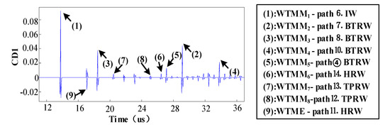
Figure 2.
Wavelet-transform modulus-maxima (WTMM) of the aerial-mode traveling wave (TW).
If a TW propagates through the full path of a branch (several branches) and reflects at its terminal (their terminals), the distance difference related to this BTRW and the IW is equal to twice the length of that branch (sum of the length of those branches) in principle. Otherwise, the BTRW-IW distance difference indicates the fault distance measured from the faulted branch terminal. Using observable BTRWs, TW propagation paths could emerge by means of path match to the given network topology.
3. A Two-Step Fault Location Scheme
3.1. Faults on the Main Line
In this paper, the main line is regarded as the shortest line between two measurement units, for example, the solid line 1–8 with two measurement units at both ends, as shown in Figure 3. Fault location on the main line can be determined by using a two-terminal approach with synchronous measurement. In Figure 3, the fault distance is simply calculated by (3).
where is the length of the main line. is the fault distance from the measurement point 1. and are the arrival time of IW obtained at measurement units 1 and 8, respectively. is the TW propagation speed. Since only the distribution network with overhead lines is studied in this paper, the propagation speed of TW in overhead lines is constant, which is close to the speed of light.
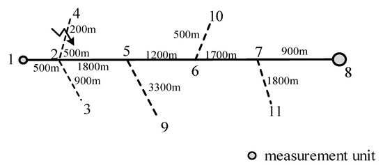
Figure 3.
A branch network with two measurement units.
Suppose that a fault occurs on the main line, for example, at tee point 2 in Figure 3. The fault-originated TW propagates directly to point 1 and point 8 in time and . Substituting and into (3), . It is evident that for any potential faults occurring on branch 2–3 or 2–4, remains the same since an identical time delay applies to and . Therefore, a fault on branch 2–3, branch 2–4, or the tee point 2 can be considered as occurring at the same location by using two synchronous measurement units if an error tolerance is allowed. Herein, a 5 m error tolerance is adopted. As a result, fault location on the main line or the faulted branch can be determined with a two-terminal method.
3.2. Faults on the Branch
If a fault occurs on the branch, the faulted branch is simply positioned following the discussion in Section 3.1. To further seek the exact fault distance, reflected TWs observed at either measurement unit and their associated WTMMs are utilized. The processing scheme is illustrated in Figure 4, where Li represents the length of all branches which are along the main line between the “faulted” tee point and the measurement unit. The reflection distance Si can be calculated by (4).
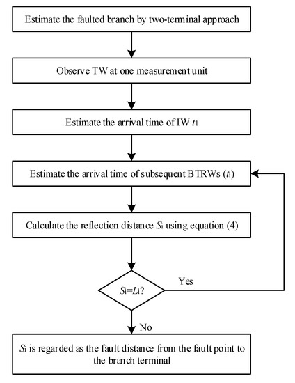
Figure 4.
Fault location on a branch.
Here, , where is the arrival time of the reflected waves and is the arrival time of the IW.
Suppose that a fault occurs 200 m away from the terminal of branch 2–4 which is 700 m in length, as shown in Figure 3.
By using the two-terminal approach, a preliminary estimation shows that the fault is probably on branch 2–3 or on branch 2–4. Then the WTMEs of the aerial-mode voltage obtained at measurement unit 1 are used to determine the fault distance. As shown in Figure 5, only positive WTMEs are employed, and these WTMMs are indexed in a descending order with respect to their magnitudes. According to Equations (1) and (2), the first few reflected waves should be the BTRWs. It is worth noting that the path search will speed up if starting from the branch terminals.
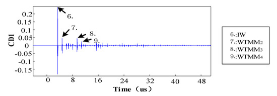
Figure 5.
Wavelet-transform modulus-extremum (WTME) of the aerial-mode TW.
In Figure 5, WTMM2 indicates a reflection at branch terminal and the distance difference with respect to the IW is 201 m, according to Equation (4). Thus, the fault probably exists at the position 201 m away from the terminal of either branch 2–4 or branch 2–3. WTMM3 also shows a reflection distance of 903 m, which corresponds to the length (900 m) of branch 2–3 (with a small error). It implies that the TW propagates from the fault location to measurement unit 1 through a reflection at point 3, thus branch 2–3 is not the faulted branch. Now, the fault is identified at the location 201 m away from the terminal of branch 2–4.
3.3. Consideration of Reducing Measurement Units in a Complex Network
This section generalizes the two-step fault location approach in a complex network. As shown in Figure 6, a multi-level branch network is divided into two sub-networks to reduce the measurement units as much as possible. The basic idea is, in each sub-network, to select a backbone along which single-level branches are attached. In this way, a few synchronous measurement units can be easily applied in each sub-network. The result is shown in Figure 7, where the two sub-networks require four measurement units at points 1, 8, 14, and 18. It has to be noted that the sub-networks may have the same backbone sections such as the Section 3 and Section 4 in Figure 7a,b. The principle to deploy measurement units is summarized as the following.
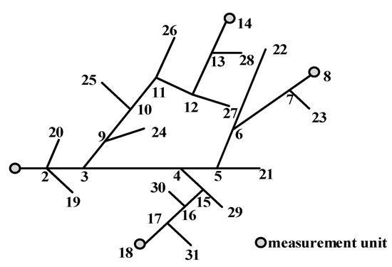
Figure 6.
A multi-level branch distribution network.
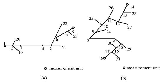
Figure 7.
Network separation. (a) sub-network with two measurement units at 1 and 8; (b) sub-network with two measurement units at 14 and 18.
- (1)
- Put one measurement unit at the substation.
- (2)
- Search for one tee point in the direction outward from the substation.
- (3)
- Observe whether this tee point is connected to another tee point in the outward direction. If the result is positive, move on to the next tee point.
- (4)
- Observe whether this tee point is connected to the terminated branches. If the result is positive, put one measurement unit at any branch end.
- (5)
- Complete measurement unit deployment after all the tee points are considered.
4. Simulation Results
In order to validate the proposed approach, a real 10 kV distribution network in China has been modeled in PSCAD/EMTDC. The network topology is shown in Figure 8, where a 110 kV/10 kV step-down transformer is used with its neutral grounded through an arc suppression coil. The load transformer is in Yyn mode. Frequency-dependent model is used for the overhead lines. In the following simulations, the sampling rate of each measurement unit is set as 50 MHz.
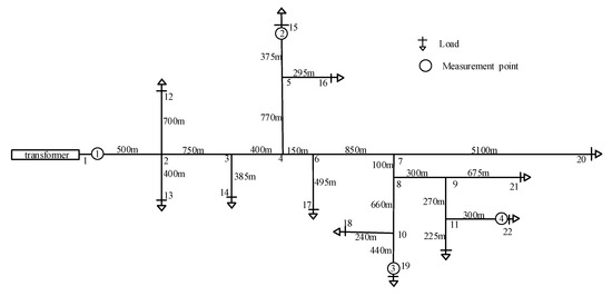
Figure 8.
Topology of a real 10 kV distribution network.
4.1. Measurement Units Deployment
Usually, one measurement unit is fixed at the substation for data collection. As shown in Figure 8, point 1 is configured with a measurement unit and this point is connected to tee point 2. Since the length of each terminated line section (section 1–2/2–12/2–13) is different, only one measurement unit is needed for this tee point. Then, for the next tee point 3, which connects two tee points 2 and 4, the measurement unit is not needed. Similarly, it is not necessary to deploy a measurement unit for tee point 4, which connects tee point 3, 5, and 6. However, one measurement unit is required at terminal 15 (or 16) because tee point 5 connects one tee point 4 and two branch terminals 15 and 16. As a result, measurement units are deployed at the branch terminals 1, 15, 19, and 22, and the entire network can be divided into two sub-networks as shown in Figure 9.
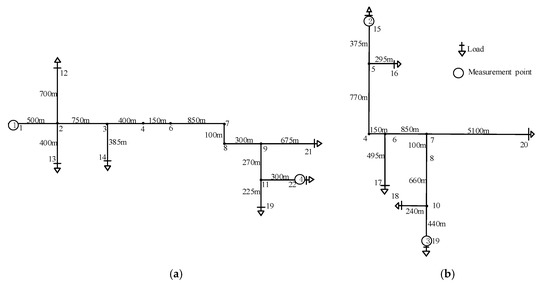
Figure 9.
Sub-networks derived from Figure 8. (a,b) are two divided sub-networks.
4.2. Single-Phase-to-Ground Fault at Different Locations
(1) Assume that a phase B-to-ground fault occurs at the position 225 m away from the terminal of branch 3-14, as shown in Figure 9a. The fault starts at 0 s. The voltage TW measured at measurement unit 1 and 4 and their aerial-mode components are shown in Figure 10. The db4 mother wavelet is used to decompose the aerial-mode voltage, and the coefficients of the first level (CD1) are employed for analysis as shown in Figure 11.
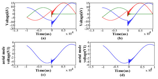
Figure 10.
The voltage TWs and their aerial-mode components for a phase-to-ground fault on the branch. (a) The voltage TW measured at measurement unit 1; (b) The voltage TW measured at measurement unit 4; (c) The aerial-mode component of (a); (d) The aerial-mode component of (b).
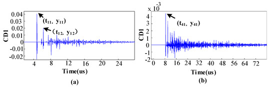
Figure 11.
The coefficient of the first level (CD1) component of aerial-mode voltage of Figure 10. (a) The CD1 at measurement unit1; (b) The CD1 at measurement unit 4.
With the obtained CD1 components, fault location can be determined through two steps as the following.
Step 1: Fault position on the main line or the tee point related to the faulted branch can be identified by the IW’s arrival time at two measurement units, such as t11 and t41, shown in Figure 11a,b.
In Figure 11, t11 is 4.76 indicating the arrival time of the IW at measurement unit 1, and t41 is 8.52 indicating the arrival time of the IW at measurement unit 4. The direct path between measurement unit 1 and measurement unit 4 is 3620 m in length. According to Equation (3), the estimated fault distance is 1246 m away from measurement unit 1. Since the length of Section 1 and Section 2 plus Section 2 and Section 3 is 1250 m, which is close to the estimated fault distance, it may result in an ambiguity. Now, it is uncertain whether the fault is on the main line or on the branch. In this case, a further step is required.
Step 2: The exact fault position on the possible faulted branch can be determined by reflected TWs obtained at a single measurement unit.
In Figure 9a, TWs measured at measurement unit 1 are used to calculate the fault distance on the faulted branch. As shown in Figure 11a, t11 (4.76 ) and t12 (6.28 ) correspond to WTMM1 and WTMM2 respectively. The reflection distance is calculated as 228 m by using Equation (4). This result is not the same length as of any sections between measurement unit 1 and tee point 3, such as branch 2–12 and 2–13. Therefore, the fault is on branch 3–14 and 228 m to its terminal, which is slightly different from the true fault distance.
(2) Assume that a phase B-to-ground fault occurs at tee point 3 as shown in Figure 9a. The fault occurs at 0 s. The voltage TW measured at point 1 and 4 and their aerial-mode components are shown in Figure 12. The CD1 components are shown in Figure 13.
Figure 12.
The voltage TWs and their aerial-mode components for a phase-to-ground fault at tee point 3. (a) The voltage TW measured at measurement unit 1; (b) The voltage TW measured at measurement unit 4; (c) The aerial-mode component of (a); (d) The aerial-mode component of (b).
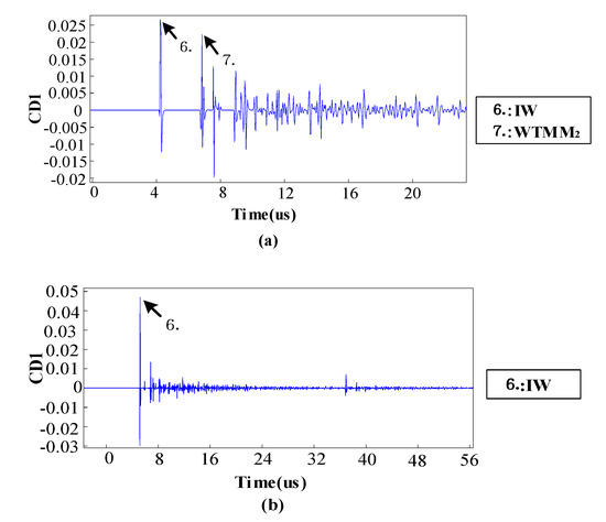
Figure 13.
The CD1 component of aerial-mode voltage of Figure 12. (a) The CD1 at measurement unit 1; (b) The CD1 at measurement unit 4.
The tee point 3 is first identified as a possible fault location by using the two-terminal approach as mentioned above (see Figure 13a,b). Then, at measurement unit 1, the reflection distance is calculated with respect to the time difference of IW and WTMM2 as shown in Figure 13a. The result is 384.5 m, which is almost the same length of branch 3–14, thus the fault is located at tee point 3.
(3) Assume that a phase B-to-ground fault occurs at 4750 m to the terminal of branch 7–20 as shown in Figure 9b. The fault occurs at 0 s. This fault happens far away from the branch terminal, and the WTMM of the BTRW is much smaller than that of the IW. The voltage TW obtained at measurement unit 2 and 3 and their aerial-mode components are shown in Figure 14 and their CD1 components are shown in Figure 15.
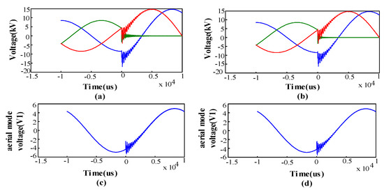
Figure 14.
The voltage TWs and their aerial-mode components for a phase-to-ground fault on a long branch. (a) The voltage TW measured at measurement unit 2; (b) The voltage TW measured at measurement unit 3; (c) The aerial-mode component of (a); (d) The aerial-mode component of (b).
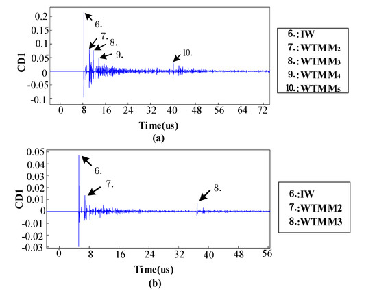
Figure 15.
The CD1 component of aerial-mode voltage of Figure 14. (a) The CD1 at measurement unit 2; (b) The CD1 at measurement unit 3.
The distance from the fault point to measurement unit 2 is estimated as 2146.5 m by using the two IWs shown in Figure 15a,b. The difference between the calculated result and the exact length from tee point 7 to measurement 2 is less than 5 m. Considering an error tolerance, the fault is probably occurring on branch 7–20 or on the main line around tee point 7, as illustrated in Figure 9b. To distinguish the false position, several reflected TWs are taken into account.
Regarding a single measurement unit (unit 2), as shown in Figure 15a, the time difference between IW and WTMM2 results in a distance difference of 294 m, which corresponds to the length of branch 5–16 in Figure 9b. Similarly, the reflection distance related to WTMM3 is 498 m which indicates the length of branch 6–17. Sometimes, the reflection distance happens to be the summed length of several individual branches. For example, the reflection distance related to WTMM4 is 792 m, which approximates the sum of the length of branch 6–17 and branch 5–16. In this way, until a reflection distance of 4758 m is obtained by using WTMM5, the fault can be determined at the position 4758 m from the terminal of branch 7–20, and false fault locations caused by the “5 m” error are excluded.
To improve the reliability of fault location determination, the CD1 component obtained at measurement unit 3 can also be used to provide a cross-check. As shown in Figure 15b, WTMM2 produces a reflection distance of 240 m which is just the length of branch 10–18. In addition, WTMM3 gives a reflection distance of 4758 m, indicating the fault location on branch 7–20. This result is the same as the one obtained at measurement unit 2.
4.3. Accuracy of the Two-Step Fault Location Approach
For the fault occurring at the tee points in Figure 8, the resulting fault location is depicted in Table 2. The relative error is calculated by (5).
where and are the real and estimated distance from the fault point to the measurement unit.
Table 2.
Fault location at different tee points.
In Table 2, the maximal absolute error of fault location is 4.5 m. If such accuracy is not satisfied, a further process is required to determine whether the fault is on a branch by using the second step of the proposed approach. In practice, such an accuracy provides an identification of fault location around the tee point, and the actual fault location can be easily determined through an operator’s inspection on site.
In the case of phase-to-ground fault on the branch, fault location results are illustrated in Table 3. The maximal relative error is 0.83%.
Table 3.
Fault location for fault on the branch.
5. Conclusions
This paper presents a traveling wave-based two-step method for phase-to-ground fault location in non-effectively earthed distribution systems. Fault location on the main line is determined by using the traditional two-terminal approach. Fault on the branch is located based on the characteristic of both amplitude and polarity of the wavelet transform coefficient of the aerial-mode traveling wave. The two-terminal step provides an overview of the potential fault locations and determines the exact fault location on the main line, or the target branches. The second single-ended step concentrates on the target branches to identify the true faulted branch and fault distance. This two-step approach takes into account both incident wave and reflected waves to improve the locating accuracy. Simulation results show that it can reach an accuracy of 5 m absolute error for a phase-to-ground fault that occurs at different positions in a multi-level branch distribution network. Combined with topology division, only one pair of measurement units is required in every sub-network, which greatly reduces the number of deployed measurement units. In addition, this two-step approach can be straightforwardly extended to other types of faults, such as phase-to-phase fault and three-phase fault, due to the fact that these faults exhibit more salient fault features.
Author Contributions
Conceptualization, T.Z.; data curation, T.Z., Y.W. and C.Y.; formal analysis, T.Z., Y.W. and C.Y.; funding acquisition, T.Z.; investigation, T.Z., Y.W. and C.Y.; methodology, T.Z. and Y.W.; project administration, T.Z. and L.Y.; resources, T.Z.; software, T.Z. and Y.W.; validation, T.Z. and L.Y.; visualization, Y.W. and C.Y.; writing—original draft, Y.W. and C.Y.; writing—review and editing, L.Y., Y.W. and C.Y. All authors have read and agreed to the published version of the manuscript.
Funding
This work was supported in part by the Key Project of Smart Grid Technology and Equipment of National Key Research and Development Plan of China under Grant 2017YFB0902900.
Conflicts of Interest
The authors declare no conflict of interest.
Abbreviations
| BTRW | Branch terminal reflected waves |
| CD1 | Coefficients of the first level decomposition through db4 wavelet transform |
| EMTR | Electromagnetic time-reversal |
| GPS | Global positioning system |
| HRW | Hybrid reflected waves |
| IW | Initial wave |
| TPRW | Tee Point or Fault Point Reflected Waves |
| TW | Traveling-wave |
| WTME | Wavelet-transform modulus-extremum |
| WTMM | Wavelet-transform modulus-maxima |
References
- Mora-Flòrez, J.; Meléndez, J.; Carrillo-Caicedo, G. Comparison of impedance based fault location methods for power distribution systems. Electr. Power Syst. Res. 2008, 78, 657–666. [Google Scholar] [CrossRef]
- Das, S.; Karnik, N.; Santoso, S. Distribution Fault-Locating Algorithms Using Current Only. IEEE Trans. Power Deliver. 2012, 27, 1144–1153. [Google Scholar] [CrossRef]
- Krishnathevar, R.; Ngu, E.E. Generalized Impedance-Based Fault Location for Distribution Systems. IEEE Trans. Power Deliver. 2012, 27, 449–451. [Google Scholar] [CrossRef]
- Salim, R.H.; Salim, K.C.O.; Bretas, A.S. Further improvements on impedance-based fault location for power distribution systems. IET Gen. Transm. Distrib. 2011, 5, 467–478. [Google Scholar] [CrossRef]
- Gong, Y.; Guzmán, A. Integrated Fault Location System for Power Distribution Feeders. IEEE Trans. Ind. Appl. 2013, 49, 1071–1078. [Google Scholar] [CrossRef]
- Salim, R.H.; Resener, M.; Filomena, A.D.; de Oliveira, K.R.C.; Bretas, A.S. Extended Fault-Location Formulation for Power Distribution Systems. IEEE Trans. Power Deliver. 2009, 24, 508–516. [Google Scholar] [CrossRef]
- Alwash, S.F.; Ramachandaramurthy, V.K.; Mithulananthan, N. Fault-Location Scheme for Power Distribution System with Distributed Generation. IEEE Trans. Power Deliver. 2015, 30, 1187–1195. [Google Scholar] [CrossRef]
- Majidi, M.; Arabali, A.; Etezadi-Amoli, M. Fault Location in Distribution Networks by Compressive Sensing. IEEE Trans. Power Deliver. 2015, 30, 1761–1769. [Google Scholar] [CrossRef]
- Saha, M.M.; Izykowski, J.J.; Rosolowski, E. Fault Location on Power Networks; Springer: London, UK, 2010; ISBN 978-1-84882-886-5. [Google Scholar]
- Sadeh, J.; Bakhshizadeh, E.; Kazemzadeh, R. A new fault location algorithm for radial distribution systems using modal analysis. Int. J. Electr. Power Energy Syst. 2013, 45, 271–278. [Google Scholar] [CrossRef]
- Borghetti, A.; Corsi, S.; Nucci, C.A.; Paolone, M.; Peretto, L.; Tinarelli, R. On the use of continuous-wavelet transform for fault location in distribution power systems. Int. J. Elect. Power Energy Syst. 2006, 28, 608–617. [Google Scholar] [CrossRef]
- Borghetti, A.; Bosetti, M.; Nucci, C.A.; Paolone, M.; Abur, A. Integrated Use of Time-Frequency Wavelet Decompositions for Fault Location in Distribution Networks: Theory and Experimental Validation. IEEE Trans. Power Deliver. 2010, 25, 3139–3146. [Google Scholar] [CrossRef]
- Razzaghi, R.; Lugrin, G.; Manesh, H.; Romero, C.; Paolone, M.; Rachidi, F. An Efficient Method Based on the Electromagnetic Time Reversal to Locate Faults in Power Networks. IEEE Trans. Power Deliver. 2013, 28, 1663–1673. [Google Scholar] [CrossRef]
- Borghetti, A.; Bosetti, M.; Di Silvestro, M.; Nucci, C.A.; Paolone, M. Continuous-Wavelet Transform for Fault Location in Distribution Power Networks: Definition of Mother Wavelets Inferred from Fault Originated Transients. IEEE Trans. Power Syst. 2008, 23, 380–388. [Google Scholar] [CrossRef]
- Shi, S.; Zhu, B.; Lei, A.; Dong, X. Fault Fault Location for Radial Distribution Network via Topology and Reclosure-Generating Traveling Wave. IEEE Trans. Smart Grid. 2020, 10, 6404–6413. [Google Scholar] [CrossRef]
- Lopes, F.V.; Dantas, K.M.; Silva, K.M.; Costa, F.B. Accurate Two-Terminal Transmission Line Fault Location Using Traveling Waves. IEEE Trans. Power Deliver. 2018, 33, 873–880. [Google Scholar] [CrossRef]
- Korkali, M.; Abur, A. Optimal Deployment of Wide-Area Synchronized Measurements for Fault-Location Observability. IEEE Trans. Power Syst. 2013, 28, 482–489. [Google Scholar] [CrossRef]
- Korkali, M.; Lev-Ari, H.; Abur, A. Traveling-Wave-Based Fault-Location Technique for Transmission Grids Via Wide-Area Synchronized Voltage Measurements. IEEE Trans. Power Syst. 2012, 27, 1003–1011. [Google Scholar] [CrossRef]
- Robson, S.; Haddad, A.; Griffiths, H. Fault Location on Branched Networks Using a Multiended Approach. IEEE Trans. Power Deliver. 2014, 29, 1955–1963. [Google Scholar] [CrossRef]
- Salehi, M.; Namdari, F. Fault location on branched networks using mathematical morphology. IET Gen. Transm. Distrib. 2018, 12, 207–216. [Google Scholar] [CrossRef]
- Goudarzi, M.; Vahidi, B.; Naghizadeh, R.A.; Hosseinian, S.H. Improved fault location algorithm for radial distribution systems with discrete and continuous wavelet analysis. Int. J. Electr. Power Energy Syst. 2015, 67, 423–430. [Google Scholar] [CrossRef]
- Tashakkori, A.; Wolfs, P.J.; Islam, S.; Abu-Siada, A. Fault Location on Radial Distribution Networks via Distributed Synchronized Traveling Wave Detectors. IEEE Trans. Power Deliver. 2020, 35, 1553–1562. [Google Scholar] [CrossRef]
- Xie, L.; Luo, L.; Li, Y.; Zhang, Y.; Cao, Y. A Traveling Wave-Based Fault Location Method Employing VMD-TEO for Distribution Network. IEEE Trans. Power Deliver. 2020, 35, 1987–1998. [Google Scholar] [CrossRef]
- Pourahmadi-Nakhli, M.; Safavi, A.A. Path Characteristic Frequency-Based Fault Locating in Radial Distribution Systems Using Wavelets and Neural Networks. IEEE Trans. Power Deliver. 2011, 26, 772–781. [Google Scholar] [CrossRef]
- Reddy, M.J.B.; Rajesh, D.V.; Gopakumar, P.; Mohanta, D.K. Smart Fault Location for Smart Grid Operation Using RTUs and Computational Intelligence Techniques. IEEE Syst. J. 2014, 8, 1260–1271. [Google Scholar] [CrossRef]
- Lout, K.; Aggarwal, R.K. Current transients based phase selection and fault location in active distribution networks with spurs using artificial intelligence. In Proceedings of the 2013 IEEE Power & Energy Society General Meeting, Vancouver, BC, Canada, 21–25 July 2013; pp. 1–5. [Google Scholar] [CrossRef]
© 2020 by the authors. Licensee MDPI, Basel, Switzerland. This article is an open access article distributed under the terms and conditions of the Creative Commons Attribution (CC BY) license (http://creativecommons.org/licenses/by/4.0/).