A Novel Probabilistic Approach to Optimize Stand-Alone Hybrid Wind-Photovoltaic Renewable Energy System

Abstract

In the present study, a novel probabilistic approach is proposed to optimize a stand-alone hybrid wind-photovoltaic renewable energy system installed in the South China Sea. In detail, the probability distribution of power generated from a hybrid wind-photovoltaic system is estimated based on the probabilistic descriptions of wind and solar energy resources in the South China Sea. In addition, the present study proposed a battery level coefficient model to calculate the battery capacity of the hybrid system. As the battery level coefficient implies the expected power deficit in a specific continuous duration, it reflects the reliability of the battery system and, hence, the performance of the system under the power deficit condition. Given the probabilistic models estimated the stability of power generations, a genetic algorithm is applied to optimize the sizes of the system components (the installed capacities of wind turbines and photovoltaic modules and the load) when the levelized cost of energy (LCOE) is used as the indicator. The optimization verifies that the proposed probabilistic approach provides reasonable estimates of the power generation of a hybrid system in an optimization process. In addition, the comparisons with the conventional deterministic approach implies that the widely used loss of power supply probability (LPSP) could be interpreted, in a statistical sense, as the expected duration of power deficit. More importantly, the LPSP is connected to the localized sea condition, and therefore, this stability assessment criterion should be specified according to the location where the system is installed.

1. Introduction

As one of the promising solutions in dealing with the dilemma where the energy production/consumption and environment protection should be trickily balanced, the exploitation and use of renewable energies acquired vigorous promotions from governments worldwide. Consequently, the use of renewable energies has been increased constantly in the energy consumption mix [1]. The exploitation of wind and solar energies has always been important in engineering applications, as they are the most feasible renewable energy forms currently available in the market. In 2018, wind energy, in fact, accounted for more than half of the renewable energy production, i.e., 51.2%, and solar energy accounted for 23.6% [1]. Given this trend, more and more scholars have devoted efforts to investigate the feasibility and benefits/costs of harnessing ocean renewable energies [2]. As for remote islands, telecommunication stations, airports in artificial islands, etc., the cost to connect the small-scale energy consumption to the power grid is unacceptably high [3]. Therefore, it is ideal to establish an offshore wind farm in the sea area nearby and supply the energy directly to the consumption occurring on remote islands/platforms.

Compared to the inland wind energy, offshore wind resources are more abundant, and the construction of wind farms has less impact on the environment. In addition, the noise pollution alleviates when the wind turbine moves from inland sites to offshore sites. The installation cost for an offshore wind farm is, however, significantly higher than its inland counterparts [4]. Consequently, it is suggested that the platforms supporting offshore wind turbines could be used to integrate photovoltaic power (PV) generation systems. For one thing, the integration of PV power generation compensates the fluctuations in the power generated by winds and, hence, increases the operability of the integrated system. For another thing, the integration of the PV generation system shares the installation cost of the support platform and, hence, lowers the levelized cost of energy (LCOE) of the power generated. In fact, the introduction of PV generation to an offshore wind farm to build a stand-alone hybrid wind-PV system (HWPS) has attracted attention from scholars with various backgrounds and is now a new direction in planning and constructing offshore wind farms [2,5].

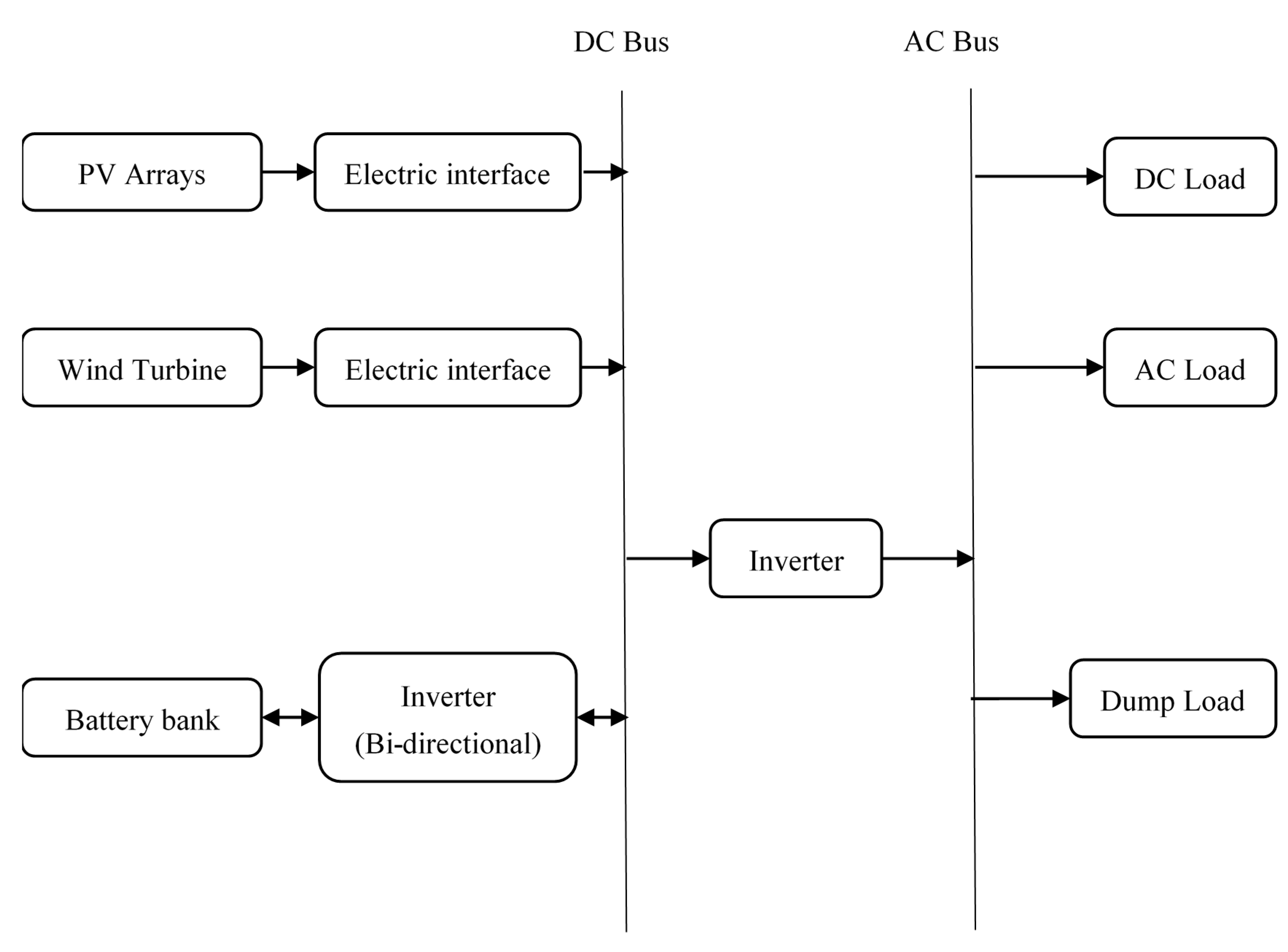
The topology of the stand-alone HWPS with batteries is shown in Figure 1. The wind turbine and the PV array are the power generation modules, and the battery is considered as a buffer module. Via the central controlling module, the power generated form of the HWPS matches, in a statistical sense, the consumption in the entire lifetime of the system. Conventionally, there are two indices evaluating the performance of the HWPS, i.e., the stability of power generations and the LCOE of the power supply. It is well-established that these indices are contradictive [6]. Therefore, it is necessary to find an optimal configuration that balances the requirements of stable power generations and comparatively low installation and operation costs. Generally, the optimal configuration is obtained through finding the lowest LCOE under the constraint that the power generation should be stable and satisfies the power consumption. According to the approach of estimating the power generation stability, the optimization of the HWPS configuration could be categorized into either the deterministic method, which is based on the observed/modeled temporal wind/solar data, or the probabilistic method, which is based on the statistical characteristics of the wind and PV resources. More specifically, the deterministic approach directly uses the meteorological time series data, such as wind speeds and solar irradiation, taken from observations or mesoscale models. Since the deterministic approach is intuitive and more reliable, given the accurate observed/modeled time series of the meteorological variables, it is the mainstream in assessing the performance of a HWPS. The probabilistic approach, on the other hand, takes all the variables involved in the energy conversion process as random variables, calculates the corresponding probability density function (PDF), and then estimates the power generation stability in the optimization of the HWPS.

There is a considerable amount of studies using the deterministic approach to estimate the power generation stability of a HWPS. For example, Borowy et al. [7] introduced the theory of loss of the load probability to determine the reliability level of a HWPS. Kellogg et al. [8] proposed the standard of using the loss of power supply probability (LPSP) to measure reliability the hybrid system. More specifically, Yang et al. [9,10] developed an optimization algorithm to find the configuration of a HWPS connected to a telecommunication station located on an island. Ma et al. [3] carried out a systematic technoeconomic analysis on the establishment of a stand-alone HWPS on a remote island and conducted a sensitivity analysis on the key parameters determining the configuration of the HWPS. Askarzadeh [11] investigated the addition of tidal energy devices to a conventional HWPS. In fact, he used the crow search algorithm to find the optimal combination of the three-phase system and concluded that tidal energy can reduce the overall installation and maintenance cost of the hybrid system. Chen et al. [12] discussed the impacts of the operation scheduling strategy on the optimization of a HWPS and found that different criteria assessing the power generation stability could lead to different optimization results. Compared to the deterministic approach, fewer literature employed a probabilistic concept in the optimization of the HWPS. Tina et al. [13], for instance, suggested that probability distributions could be used to describe statistical characteristics of wind speeds and solar irradiance, which could then be used to evaluate the long-term performance of HWPS via convolution techniques. Through comparing the evaluations resulted from probabilistic models and from the time domain data, Tina et al. concluded that the probabilistic approach is equivalent to the deterministic method in terms of evaluating the stability of power generations. Tina et al. [14] used the observation data taken at the Pennisi College in Italy to reveal the necessity of using probability models to preprocess the data of wind speeds and solar irradiance for the evaluation of a HWPS. Arabali et al. [15] used probability distributions to model wind speeds, solar irradiance, and loads in a study optimizing the HWPS to supply the consumption of an air ventilation system. Maghraby et al. [16] studied the reliability of a PV system, in terms of power generations, located in remote offshore areas via stochastic models. Via comparing three models estimating the power generation reliability, i.e., fixed autonomous days, loss of load probability, and Markov chain, they found that the loss of load probability method significantly reduced the number of photovoltaic panels and batteries, which lead to lower installation and maintenance costs.

The main disadvantage of the deterministic approach is that the historical data is regarded as the “deterministic” in projecting the performance of a HWPS in the future without considering the randomness of the historical data. Some studies [17] have demonstrated that, due to the chaotic nature of meteorological events, the recorded data may bear significant deviations, in a statistical sense, between current and future measurements. In addition, the reliability of the projection made based on the deterministic approach relies on the quality of the input temporal series. In many areas (such as the sea areas near the islands and reefs in the South China Sea), the complete and detailed measurement is absent and, consequently, limits the application of the deterministic method. Different from the deterministic approach, the probabilistic approach does not directly rely on a long-term observational/modeled time series. Instead, the reliability of the projections is connected to the accuracy of a few model parameters of the PDFs associated with meteorological variables. While a piece of contaminated data in the time series could lead to the unreliable near-future prediction of the HWPS made by the deterministic method, its influence on the probabilistic model parameters is limited. In addition, the long-term projection based on the probabilistic model could be made using just a small fraction of the historic data with sufficient representativeness. For example, Ding et al. [18] used the monthly wind speed data to fit the Weibull distribution parameters and then predicted the corresponding monthly distribution parameters in the future through the grey model. The results showed that using less historical data could, surprisingly, obtain a higher prediction accuracy.

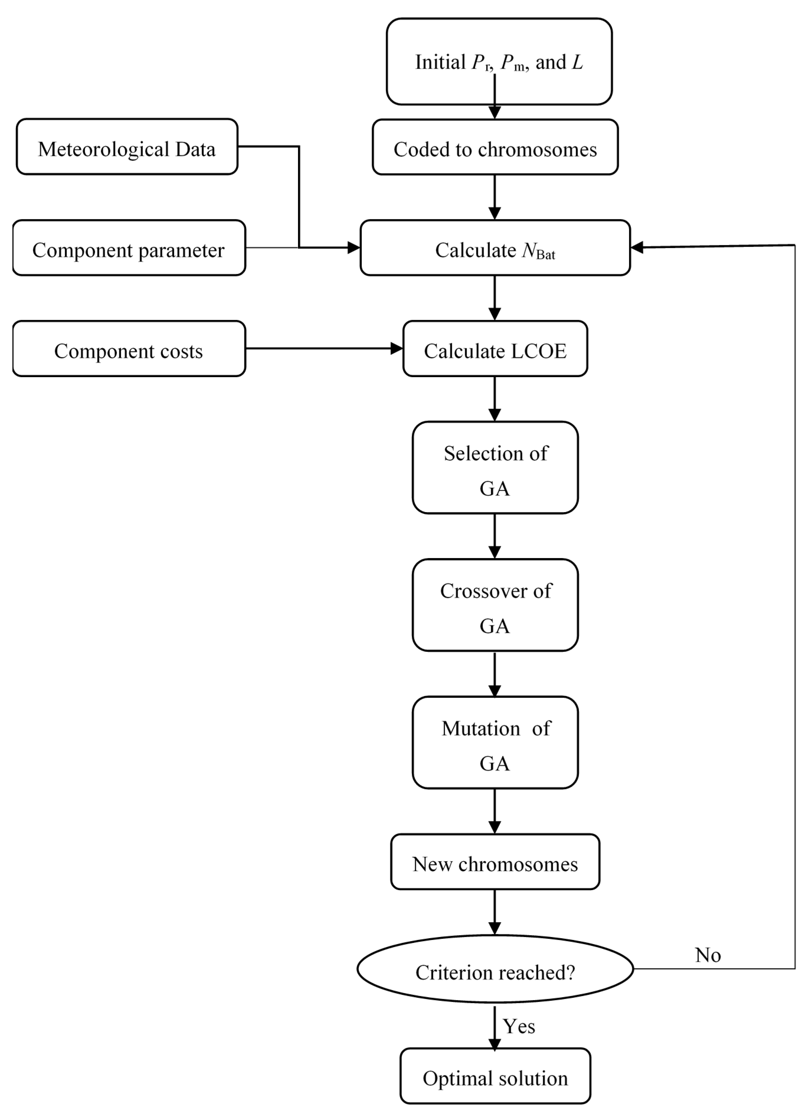
An innovative optimization algorithm, which is based on probabilistic descriptions of the wind speeds and solar irradiance, is proposed in the present study. In addition, the present study introduces a new concept describing the battery capacity, i.e., the battery level coefficient, of the HWPS. Via probabilistic models describing the performance of power generation and buffer modules, the stability of the power supplied from the HWPS system is analyzed. Given the constraint of the power supply stability, the genetic algorithm (GA) is used to optimize the configuration of the HWPS corresponding to the lowest LCOE. The main contributions of the present study are:

• A novel algorithm is proposed to optimize the configuration of the HWPS based on the statistical descriptions of wind speeds and solar irradiance.
• A new battery level coefficient is proposed to model the battery storage statistically.
• The HWPSs at four selected sites in the South China Sea are optimized via the novel algorithm to verify the proposed approach.
• A new interpretation of the LPSP criterion is proposed based on the statistical descriptions of the wind speeds, solar irradiance, and the battery capacity.

Following the Introduction, Section 2 describes the models of each component in the HWPS. In Section 3, the optimizations of the idealized HWPSs located in four selected sea areas in the South China Sea are presented. In addition, a sensitivity analysis of the expected power deficit days, which is a key in the calculation of the battery level coefficient, is carried out in Section 4. Section 5 summarizes the findings made in the present study.

2. System Model

The stand-alone HWPS is mainly composed of wind turbines, PV arrays, the battery bank, the inverter, the control unit, and the consumption load. Some hybrid systems may also contain backup power resources (such as a small-scale diesel generator), dump load, and other additional modules. Wind turbines and PV arrays are connected with the inverter through the appropriate electric interface, and the power is supplied to the consumption through the control unit. The battery is connected to the control unit as a buffer, which stores the surplus energy when the production exceeds the load and provides the deficit energy. The present study focuses on the optimal configuration of the power generation in a HWPS and, consequently, ignores the inverter and control unit in the optimization, as they are irrelevant in determining the sizes of wind turbines, PV arrays, and the battery bank. Conventionally, the optimization of the HWPS requires a predefined and constant load L. Such an optimization aims to provide the lowest LCOE of the power generated from the HWPS to supply a known consumption. In an overall optimization study, the load itself should be taken as a variable. Although the resulting optimal configuration may not satisfy the requirement of a specific offshore structure, it provides worthwhile insights into siting the offshore HWPS system. Consequently, the wind turbine installed capacity P_r, the PV array installed capacity P_m, and the load L are all taken as independent variables in the optimization model articulated in the present study.

2.1. Wind Energy Model

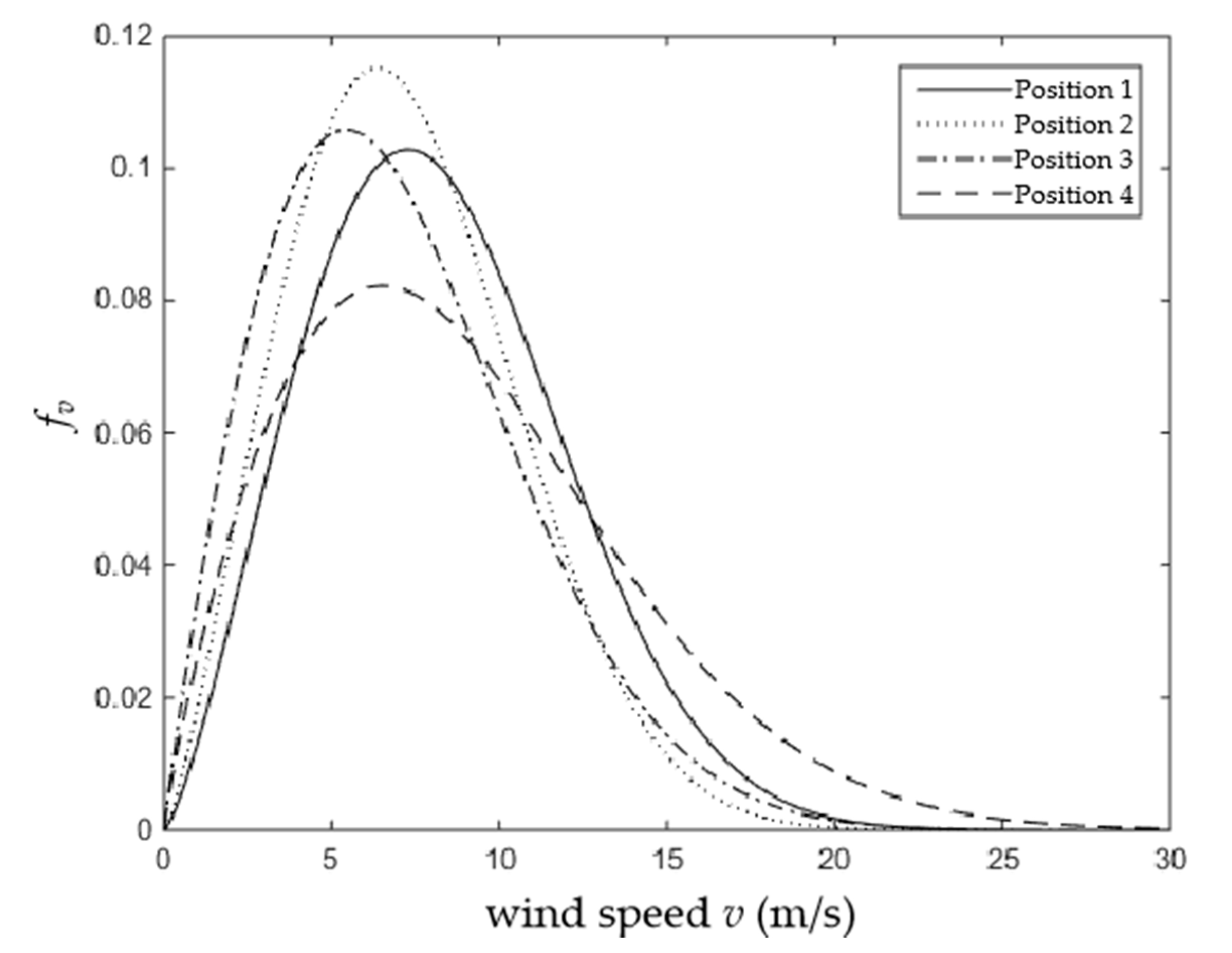
In the present study, the input parameters of wind energy module include wind speeds and the installed capacity of wind turbines, and the latter is taken as the control variable in the optimization. As regards the wind speed, the present study uses the hourly mean wind speed as an independent random variable with the identical distribution, and the Weibull model with two key parameters is used to calculate its PDF [19,20]:

$$f_v\left(v|\alpha ,\beta \right)=\frac{\beta }{\alpha }{\left(\frac{v}{\alpha }\right)}^{\beta -1}{e}^{{\left(\frac{v}{\alpha }\right)}^{\beta }}$$

(1)

In Equation (1), v is the wind speed, in the unit of m/s, and α and β are the scale parameter and shape parameter of Weibull distribution, respectively. Based on the PDF of the wind speed, there is a widely used model (wind turbine power curve) estimating the generated power as [21,22]:

$$P_{\mathrm{w}}\left(v\right)=\{\begin{array}{ll}0& v<v_{\mathrm{ci}}\\ \frac{v^m-v_{\mathrm{ci}}^m}{v_{\mathrm{r}}^m-v_{\mathrm{ci}}^m}{P}_{\mathrm{r}}& v_{\mathrm{ci}}\le v<v_{\mathrm{r}}\\ P_{\mathrm{r}}& v_{\mathrm{r}}\le v\le v_{\mathrm{co}}\\ 0& v>v_{\mathrm{co}}\end{array}$$

(2)

In Equation (2), P_w is the output power from a wind turbine, in the unit of kW; v_ci, v_r, and v_co are the cut-in, rated, and cut-off wind speeds of a specific wind turbine, respectively, in the units of m/s; P_r is the wind turbine rated power, also known as the installed capacity, in the unit of kW; and m is an empirical coefficient and takes the values of 1, 2, and 3. In the present study, m = 3 is assumed in the optimization, which is considered as the cubic power curve [21].

2.2. Solar Energy Model

The input parameters of the PV module include the solar irradiance and installed capacity of the PV array. The solar irradiance, which determines the actual output power of the PV array, is strongly related to the time in a day. For example, the solar irradiance is the strongest at noon and decreases to zero towards the night. Therefore, it is inappropriate to propose a probabilistic model directly describing the hourly mean solar irradiance as the independent random variable. In the present study, the hourly mean clearness index is used to estimate the solar irradiance. The clearness index is defined as [23]:

$$k=\frac{G}{G_0}$$

(3)

In Equation (3), k is the hourly clearness index, G is the solar irradiance at the surface in the units of W/m², and G₀ is the extraterrestrial total solar irradiance, also in the units of W/m².

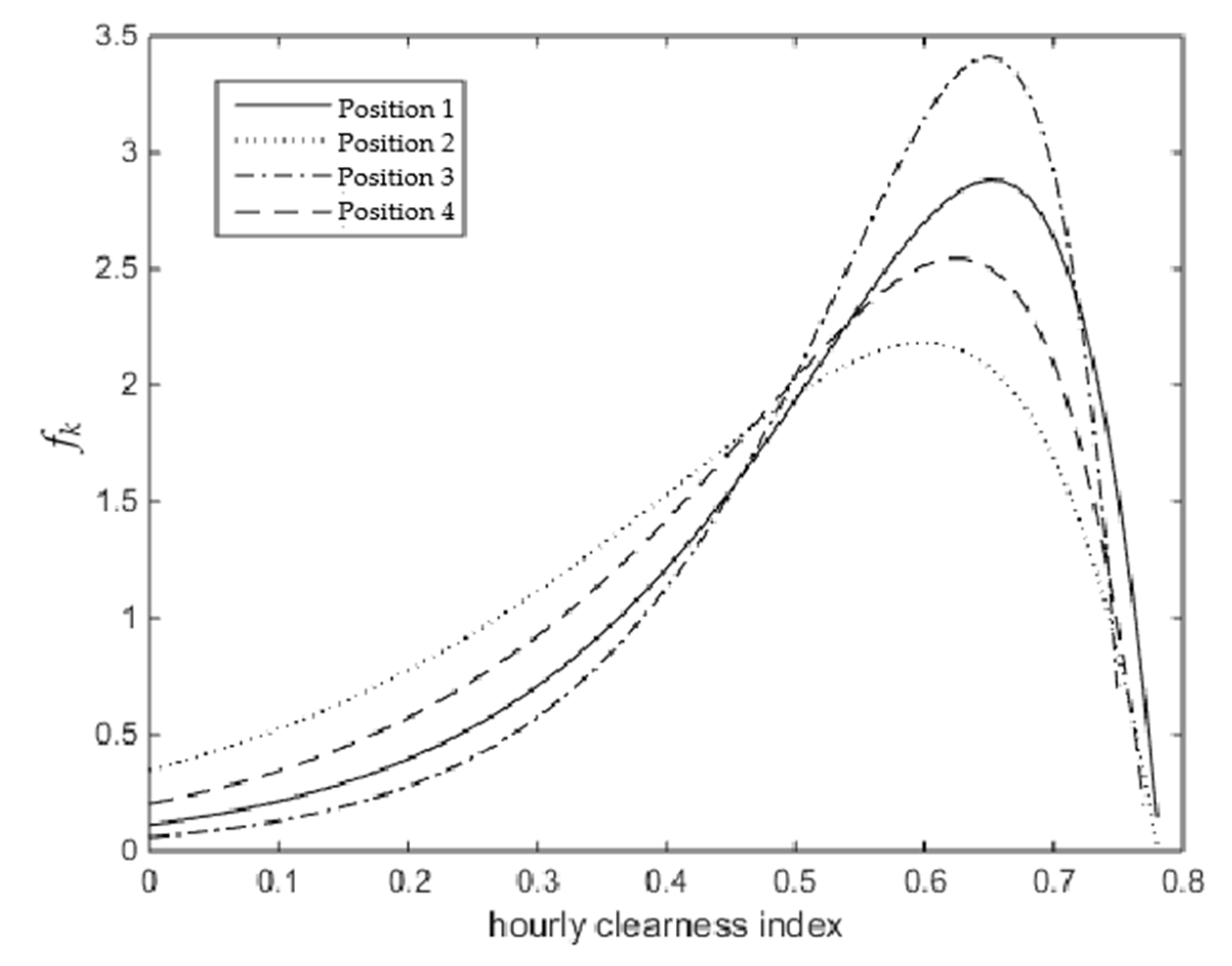
Liu et al. [24] proposed to use a function cluster to describe the probability distributions of the clearness index and found that a unique distribution model can be employed to estimate the averaged clearness index at different locations. Following this philosophy, Hollands et al. [25] proposed an improved gamma function to fit the PDF of the hourly mean clearness index and concluded that the results are in good agreement with Liu’s investigation. In the present study, the improved gamma model proposed by Hollands et al. [25] was used. More specifically, its PDF was specified as follows:

$$f_k(k|C,\lambda )=C\frac{k_u-k}{k_u}{e}^{\lambda k}$$

(4)

In Equation (4), C and λ are two model coefficients with calculations suggested by Hollands et al. [25]. $\overline{k}$ is the mean hourly clearness index, and k_u is the maximum hourly clearness index in a year. The extraterrestrial radiation G₀, on the other hand, can be calculated as [26]:

$$\begin{array}{cc}\hfill G_o& =\frac{12}{\pi }{G}_{\text{SC}}\left(1+0.033\cos \frac{360n}{365}\right)\times {10}^{-6}\hfill \\ & \times \left[\cos \varphi \cos \delta \left(\sin {\omega }_2-\sin {\omega }_1\right)+\frac{\pi \left({\omega }_2-{\omega }_1\right)}{180}\sin \varphi \sin \delta \right]\hfill \end{array}$$

(5)

In Equation (5), G_SC is the solar constant, i.e., 1367 W/m², n is the sequence number of a given day in the year, ϕ is the latitude, δ is the declination, ω₁ and ω₂ are the start hour angle and end hour angle, and T is the hour number (T = 10 in 10:00 a.m. and T = 14 in 2:00 p.m.).

From Equations (3)–(5), the solar irradiance at any given time and location can be estimated, and then, the output power of the PV arrays can be estimated [27]:

$$P_{\mathrm{s}}\left(G\right)=P_{\mathrm{m}}\frac{G}{G_{\text{STC}}}\left[1+a\left(T_{\mathrm{PV}}-T_{\text{STC}}\right)\right]\left[1-c\left(T_{\mathrm{PV}}-T_{\text{STC}}\right)\right]\left[1+b\left(\frac{G}{G_{\text{STC}}}-1\right)\right]$$

(6)

In Equation (6), P_s is the maximum output power of the PV array in the unit of W, and P_m is the maximum output power of the array under the standard test conditions, i.e., the installed capacity of the PV array, also in the unit of W. G_STC is the solar irradiation under the standard test conditions in the units of W/m², T_PV is the temperature of the PV cell in the unit of °C, and T_STC is the temperature of the PV cell under the standard test conditions, in the unit of °C. Typical values of the model coefficients a, b, and c are [27]:

$$\begin{array}{l}a=0.0025/°\mathrm{C}\\ b=0.5\\ c=0.00288/°\mathrm{C}\end{array}$$

(7)

2.3. Battery Bank Model

The battery bank acts as the buffer in the HWPS, which adjusts the output energy to match the constant load according to the commands from the control unit. If the battery discharges to the specified depth, and the system has no backup power supply, the HWPS would entirely shut down. Under the condition that the total power generation is sufficient in a long run, the battery buffers the power generated from the HWPS and yields a stable energy supply. Given the requirement of stability, the capacity of the battery bank is estimated to maintain the load under the power deficit conditions for a continuous period.

There are two main influencing factors in the estimation of the minimum battery capacity, i.e., the duration of the power deficit and the initial State of Charge (SoC). As regards to the duration of the power deficit, it is conventionally specified according to the needs of the end user. In the present optimization, a conservative length of three days is applied. The initial SoC of the battery bank at the beginning of any three-day period, on the other hand, is taken as a random variable in the present study. More specifically, a battery level coefficient is proposed to estimate the initial SoC. Afterwards, the total expected power deficit, accumulated in a three-day period, divides the battery level coefficient to calculate the battery capacity that would sustain the whole HWPS at the probability of 90% for three days under the continuous power deficit conditions.

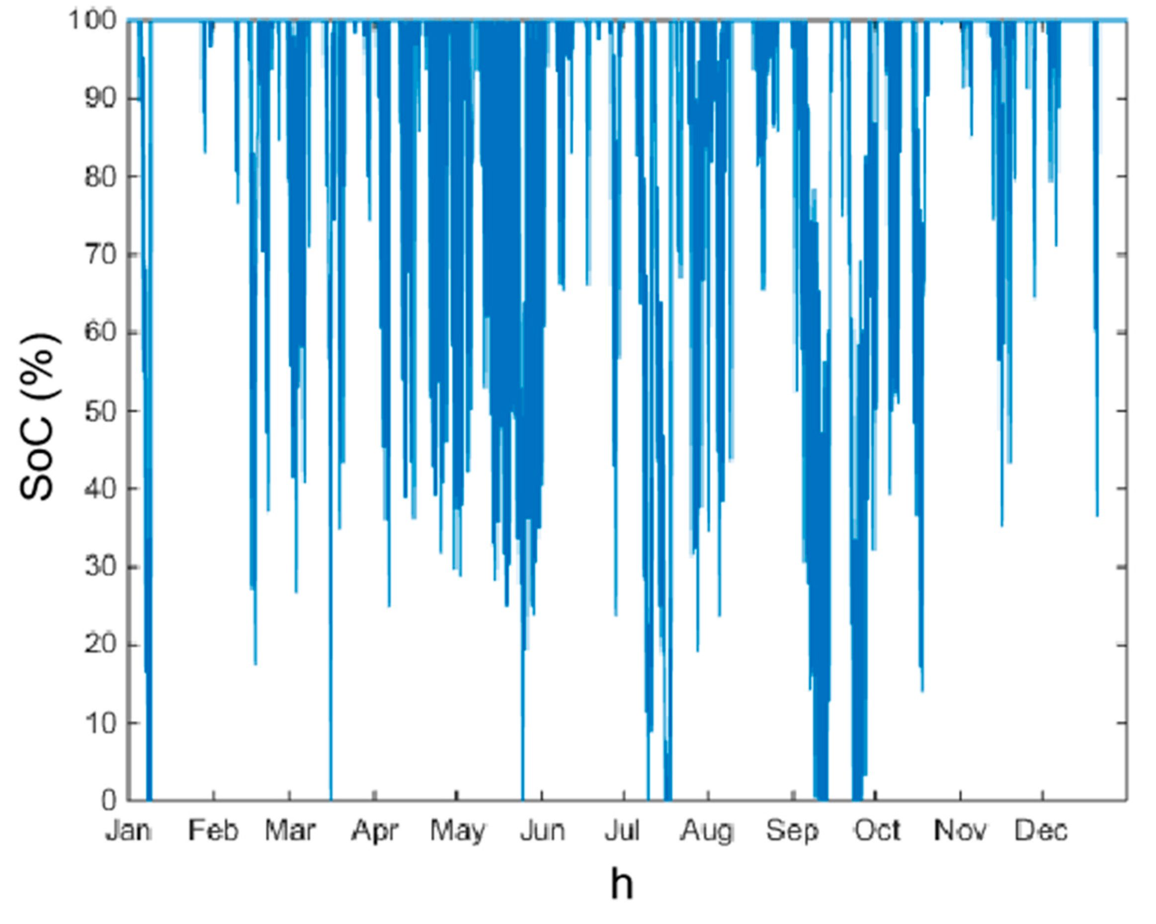
The hourly mean SoC for a typical battery bank’s works in the South China Sea in a year is shown in Figure 2.

When the hourly mean SoC in a year is taken as an independent random variable with the identical distribution, the time series of the SoC shown in Figure 2 can be employed to estimate the cumulative density function (CDF) of the SoC, as shown in Figure 3.

According to the CDF of the SoC, the quantile of 0.1, which is defined as the battery level coefficient B_f in the present study, could be calculated. As indicated by the dark square in Figure 3, the battery level coefficient in Figure 3 is B_f = 48.31%. In the present study, the HWPS with different wind turbine and PV installed capacities (P_r and P_m) and different loads (L) are simulated to provide the temporal variations of B_f. First of all, for any combination of P_r, P_m, and L, the battery pack capacity is calculated that makes the LPSP = 1% after simulation. Then, the hourly output power of the system with the specific parameters of P_r, P_m, and L is calculated. 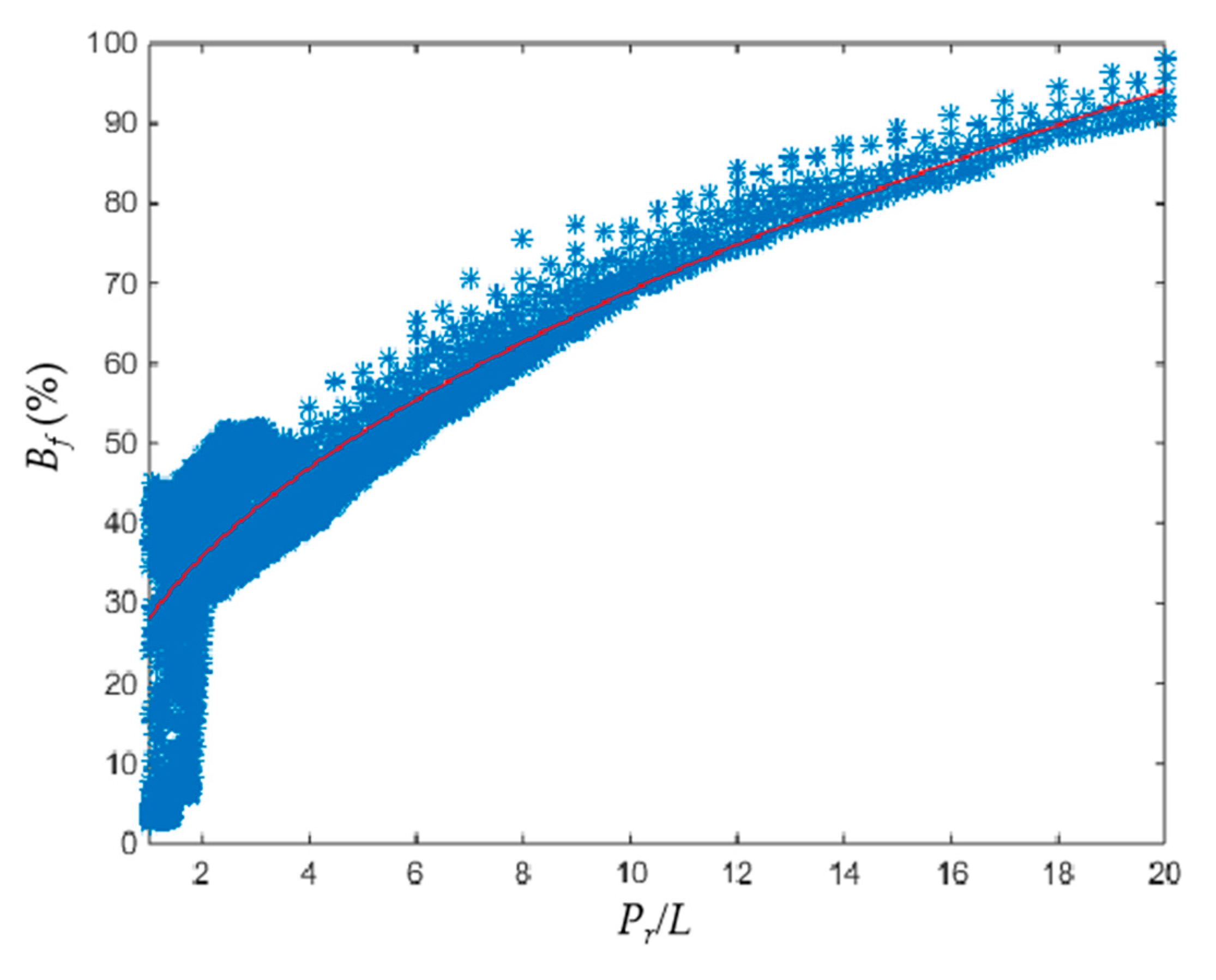Finally, the CDF of the SoC, and correspondingly, B_f, are obtained via comparing the output power and the storage capacity of the battery pack. 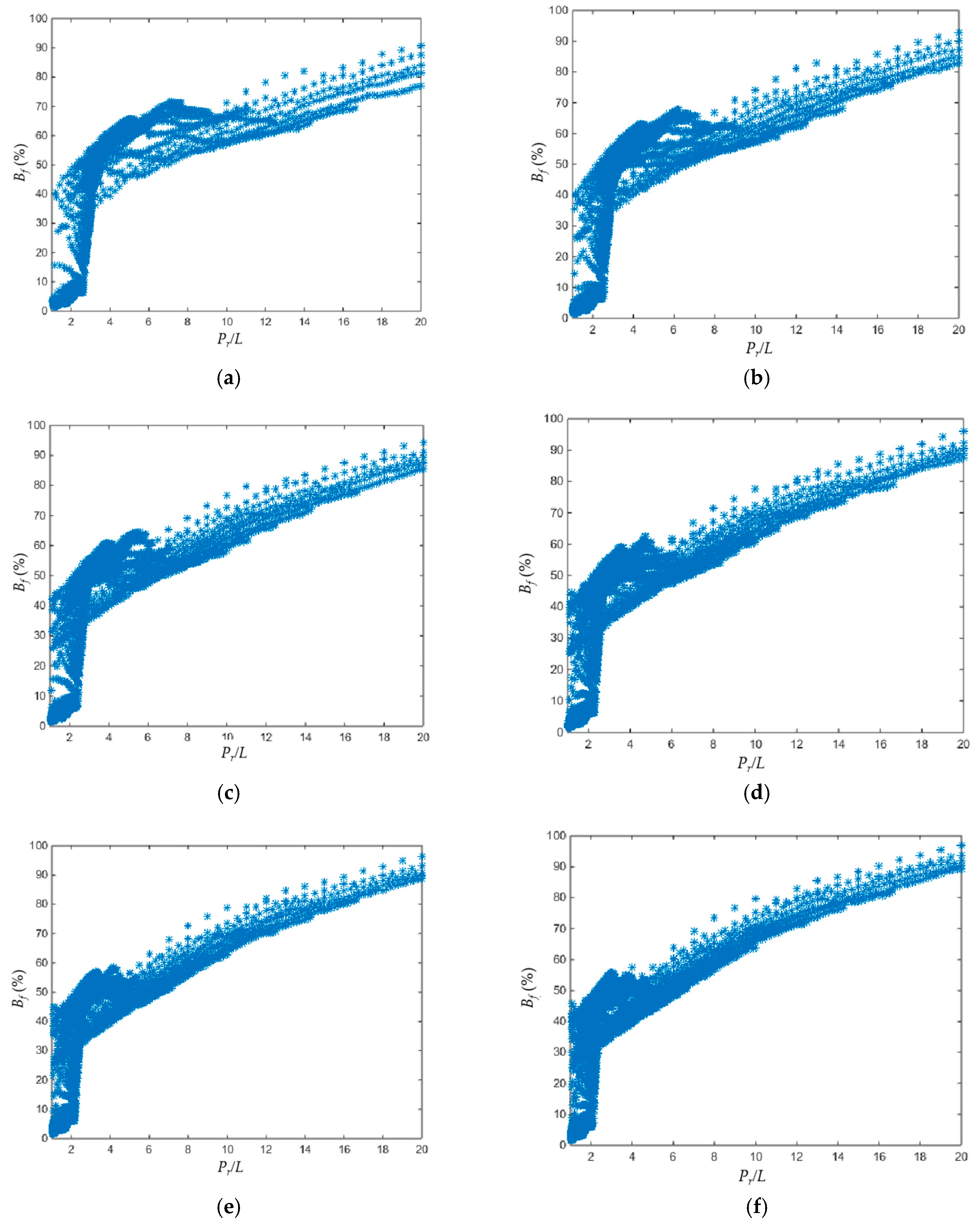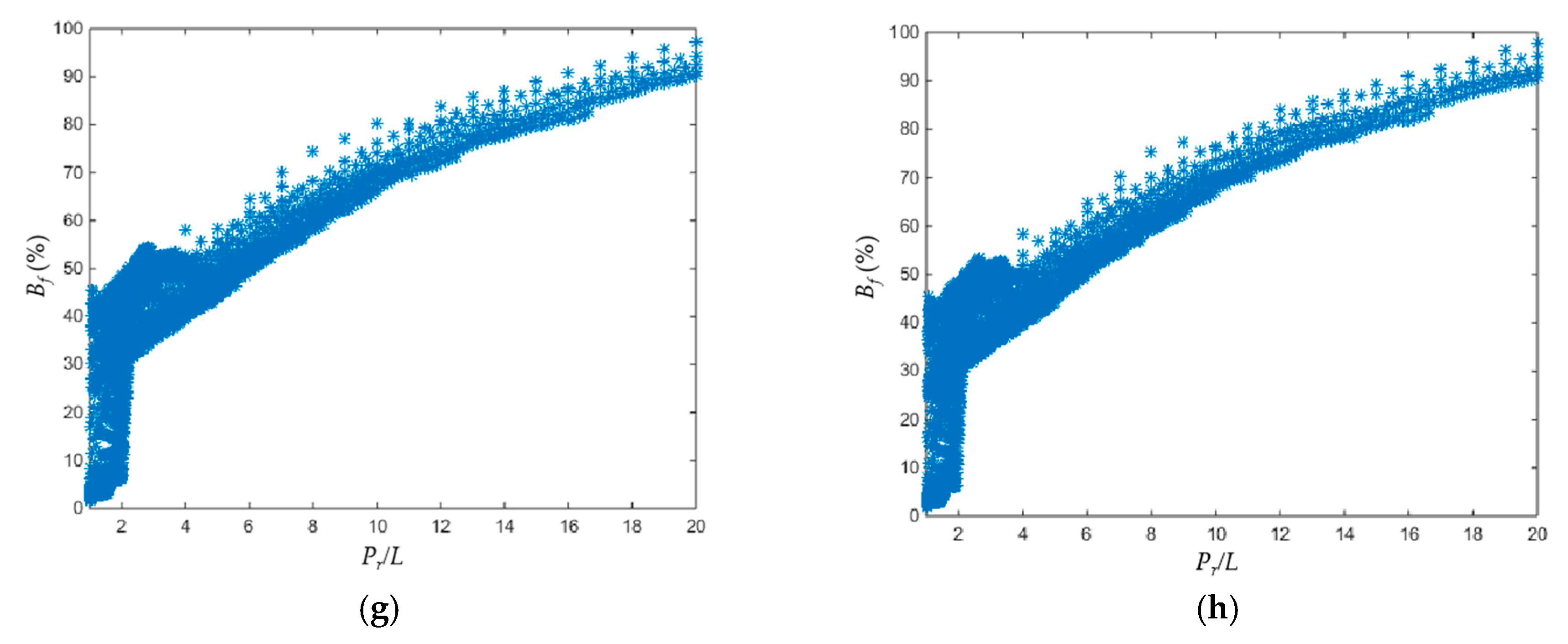It is found from the simulation results that the most influencing factor in estimating the B_f is the ratio of P_r to L, and the influence of the P_m on the B_f is relatively small. As shown in Figure 4, when the P_m varies in the range of 20kW~90kw, the scatter diagram implies that the P_m has a secondary influence on the B_f. Therefore, the present study proposes to use an exponential function to estimate the B_f based on P_r/L as:

$$B_f=B_0{\left(\frac{P_{\mathrm{r}}}{L}\right)}^{B_1}+B_2$$

(8)

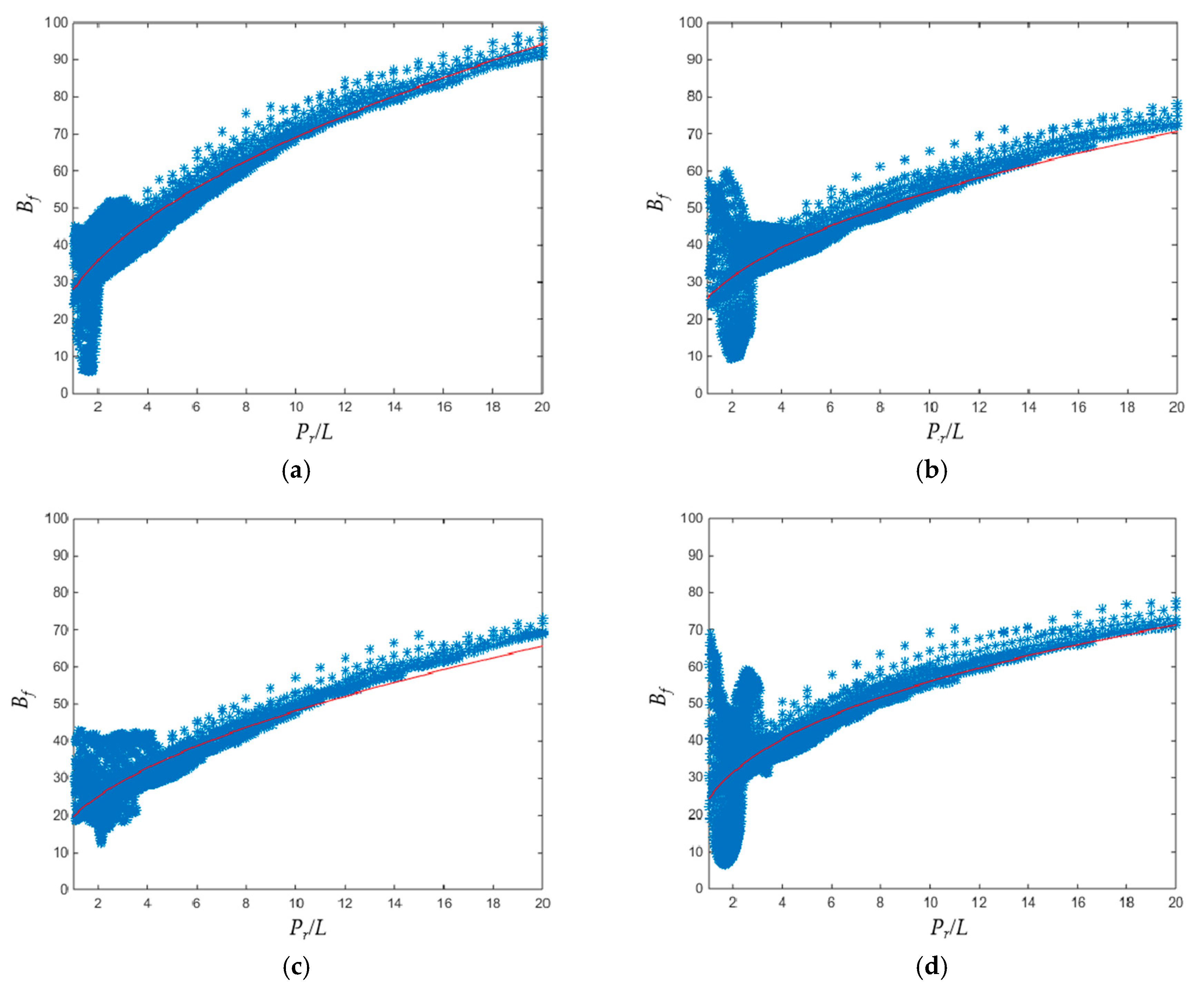
In Equation (8), L is the load in the unit of kW; B₀, B₁, and B₂ are three model coefficients related to the location in the estimation of the B_f. An example showing the modeled B_f together with the scattered B_f calculated from the simulation is Figure 5. It is evident from the figure that Equation (8) is adequate to estimate the B_f based on the ratio of the P_r/L.

2.4. Cost Model

The economic evaluation is the most important component in the feasibility assessment of a HWPS and is the most intuitive index for the investors, service providers, and other stakeholders of a HWPS. In the present study, the LCOE is used as the index and objective function in finding the optimal configuration of the HWPS. LCOE is calculated as:

$$\mathrm{LCOE}=\frac{C_{\mathrm{cap}}+C_{\mathrm{rep}}+Y{C}_{\mathrm{mai}}}{E_l\times Y}$$

(9)

In Equation (9), C_cap, C_rep, and C_mai are the initial capital cost, replacement cost, and annual maintenance cost, respectively; E_l is the annual electricity consumption in the unit of kWh; and Y is the lifetime of the project, which is taken as 20 years in the present study.

The initial capital cost is given as:

$$C_{\mathrm{cap}}=P_{\mathrm{r}}{C}_{\mathrm{WT}}+N_{\mathrm{PV}}{C}_{\mathrm{PV}}+N_{\mathrm{Bat}}{C}_{\mathrm{Bat}}$$

(10)

In Equation (10), C_WT is the initial capital cost per unit of the installed capacity of the wind turbine, N_PV is the number of PV generators in the PV array, C_PV is the initial capital cost of a single PV generator, and C_Bat is the unit cost of the battery, N_Bat is the number of battery cells.

The replacement cost is given as:

$$C_{\mathrm{rep}}=N_{\mathrm{Bat}}{C}_{\mathrm{Bat}}\left(Y/Y_{\mathrm{Bat}}-1\right)$$

(11)

In Equation (11), Y_Bat is the lifetime of the battery. Considered that both the wind turbine and PV array of the HWPS serves with no interruption in the life cycle of the HWPS (20 years), the replacement cost model discussed in the present study concerns only the replacement of batteries.

The annual maintenance cost is given as:

$$C_{\mathrm{mai}}=P_{\mathrm{r}}{C}_{\mathrm{wm}}$$

(12)

In Equation (12), C_wm is the annual maintenance cost per installed capacity for the wind turbine. Since the present study focuses on the offshore HWPS, in which the maintenance cost generally associates with the offshore operations. Such a cost can be estimated according to the known maintenance cost of installed offshore wind farms.

3. Numerical Examples

In the present study, the configuration of HWPS installed in several selected sites in the South China Sea is optimized when the LCOE is used as the objective function under the constraint of the stability requirement. The geographical locations (longitudes and latitudes) of the four selected sites (Positions 1–4) are shown in

Table 1. Information on the selected sites.

Position Number	Longitude	Latitude	Location
1	112.50E	16.75N	Near to Yongxing Island
2	115.50E	22.50N	Near to Shanwei
3	117.75E	15.25N	Near to Huangyan Island
4	119.00E	23.00N	Near to Penghu Islands

. It is noted that the selected sites are all close to either the shore of the Mainland China or small islands in the South China Sea.

3.1. Wind and Solar Energy Probability

The wind speed and solar irradiance data corresponding to the four selected sites are obtained from the ERA5 database of European Centre for Medium-Range Weather Forecasts (ECWMF) [28]. The wind speed data is the hourly mean wind speeds in the year of 2018 at the height of 10 m. The solar irradiance data is the surface solar radiation downwards per hour in the year of 2018.

It is evident from the model description in Section 2.1 that the energy output from the wind turbine is largely determined by both the wind speed statistical model and the wind turbine power curve. While it is well-established that the Weibull model is adequate to describe the statistics of wind speeds observed over land [29] and over the sea [20], there are various models estimating the wind turbine power curve. Since an optimization study requires a parametric model to estimate the energy output from a specific turbine, the linearized segmented model, polynomial model, dynamical approach, and probabilistic models are available [21]. Among the available parametric models, the manufacturer-provided power curves indicate that the cubic model (m = 3) is more appropriate to estimate the energy output from a turbine with the rated power in the range of 2.5–6 MW. In addition, the cut-in, rated, and cut-off wind speeds can be generalized as 3 m/s, 12 m/s, and 25 m/s (

Table 2. Manufacturer-provided turbine curve parameters.

Turbine	Manufacturer	Rated Power (kW)	Cut-in Speed (m/s)	Rated Speed (m/s)	Cut-off Speed (m/s)
SWT-6.0-154	SIEMENS, Germany	6000	4	13	25
FD140	DEC, China	5500	3.5	12	30
SL5000/128	Sinovel Wind Group, China	5000	3.5	12.5	25
XE/DD128	XEMC Wind Power, China	5000	3	11.5	25
G128-5.0MW Offshore	Siemens Gamesa, Spain	5000	2	14	27
GW 136/4200	Goldwind Science Technology, China	4200	2.5	11	25
E-138 EP3 E2	ENERCON GmbH, Germany	4200	2.5	10.8	34
V117-4.2 MW	Vestas, Denmark	4200	3	12	25
SWT-3.6-120	SIEMENS, Germany	3600	3.5	12	25
GW 140/3000	Goldwind Science Technology, China	3000	2.5	10.5	20
SL3000/113	Sinovel Wind Group, China	3000	3	11	25
Vensys 100	VENSYS, Germany	2500	3	11	25

).

Using the hourly mean wind speeds obtained from the ERA5 database, the parameters associated with the Weibull model are estimated via a nonlinear fitting approach. The resulting PDF curves are shown in Figure 6. When combining with the wind turbine power curve (Equation (2)), in which the key parameters are determined according to the manufacturer-provided specifications summarized in Table 2, the probability of wind turbine output powers is calculated.

In the estimation of output energy from the PV module of the HWPS, the key is the clearness index model and the PV output model (Equation (6)), as stated in Section 2.2. Although it has been asserted by Poggi et. al. that no classic probabilistic model could satisfactorily describe the statistics of solar irradiance [30], the model proposed by Hollands et al. [25] has been extensively used in assessing the performances of PV cells and describing the solar irradiances in agricultural applications [13,31,32]. Consequently, the use of Equation (4) in roughly estimating the solar irradiance in the present study is justified. The PV output model, on the other hand, is well-known to be affected by ambient temperatures, other environmental conditions, and the operation strategy of the PV panels [33]. While previous studies concern the electric details of the PV panel [31,32,33], the present study focuses on the estimates of PV output power in an optimization of the HWPS. As a general optimization study, specifications of the PV module should be standardized, and therefore, the general formulation such as Equation (6) is employed. As shown in the studies [34,35] focusing on the capacity of the PV, empirical models associating the power output with the simplified environmental parameters have commonly been utilized. Following the same philosophy, the present study optimized the configuration of a HWPS based on the standardized model calculating the PV outputs [27].

Based on the solar irradiance data from the ERA5 database, the PDF of the hourly clearness index is fitted to the model described by Equation (4), and the results are shown in Figure 7.

3.2. Battery Level Coefficient

In the case of a power deficit, the battery bank discharges to sustain the load. The capacity of the battery bank is therefore calculated according to the expected power deficit. During the first hour (t = 1) to the 6th hour (t = 6) and the 18th hour (t = 18) to the 24th hour (t = 24) of each day, solar irradiances are absent, and only the wind turbine supplies power to the load. During the 7th hour (t = 7) to 17th hour (t = 17) of each day, the wind turbine and the PV array work together to supply the power. Given the PDFs of the hourly mean wind speeds and clearness index, the expected power deficit in any given duration is estimated. Readers are suggested to refer to Appendix A for the detailed derivations. The expected power deficit is then multiplied by the corresponding time interval (three consecutive days in the present study) to obtain the expected energy shortage and the capacity of the battery.

Based on the temporal data of wind speeds and solar irradiances obtained from the ERA5 database, the present study calculates the scatter diagram of the battery level coefficient B_f corresponding to the selected sites under the condition of P_m =100 kW. Based on the scattered data, Equation (9) is employed to model the variation of the battery level coefficient B_f with the ratio of the P_r/L. The results are shown as the red curves in Figure 8.

3.3. Cost Model and Optimization Algorithm

Besides the probabilities of the wind and solar energies, the optimization employs the cost model articulated in Section 2.4, and the values of the parameters in the cost model are summarized in

Table 3. The costs for the system components. PV: photovoltaic power and WT: wind turbine.

Parameter	Variable	Value	Unit
WT initial capital cost	CWT	20,482	Yuan/kW
PV initial capital cost	CPV	2800	Yuan
Battery initial capital cost	CBat	1500	Yuan
Maintenance cost	Cwm	40	Yuan/(kW·year)

.

Based on the model calculating the output energies from the wind turbine, the PV array, and the model estimating the size of the battery bank, the productivity of the HWPS can be assessed. Combining the cost model with the productivity prediction, the LCOE of the HWPS is projected. Using the LCOE as the objective function, the configuration of the HWPS, i.e., the values of P_r, P_m, and L, are optimized under the stability constraint. Comparing to the optimization studies reported previously, the present study takes the load L as an independent variable in the optimization to find the optimal value of the load in different sites. The optimization spaces corresponding to the three variables are P_r$\in$ [0.1 MW, 50 MW], P_m$\in$ [0.1 MW, 50 MW], and L$\in$ [0.1 MW, 10 MW], respectively. The flow chart shown in Figure 9 presents the procedure to optimize the configuration of the HWPS (the values of P_r, P_m, and L).

4. Results and Analysis

The optimized results, derived based on the probabilistic models of wind speeds and solar irradiances, corresponding to the selected sites are shown in

Table 4. Optimal sizing results. P_r: wind turbine rated power, P_m: PV array installed capacity, L: load, and LCOE: levelized cost of energy.

Position Number	Pr (MW)	Pm (MW)	Es (MWh)	L (MW)	LCOE (Yuan/kWh)
1	38.43	11.23	257.7	4.40	3.9300
2	31.59	10.32	252.9	3.32	4.8780
3	48.65	12.41	319.2	4.07	5.2780
4	48.42	18.80	409.6	5.30	4.9110

. The expected power deficit for three consecutive days are also calculated and shown in Table 4 corresponding to the optimized HWPS configuration (E_s). It is evident from the table that the LCOE of the HWPS corresponding to the Position 1 is the lowest, only 3.9300 Yuan/kWh. From the perspective of the load L, the load sustained by the HWPS with the optimized configuration in Position 4 is the largest, reaching 5.3 MW. In general, the LCOE corresponding to Position 1 is the lowest, with the relatively large sustained load, which implies that Position 1 is the most suitable for the construction of an offshore HWPS. The LCOE of the HWPS in Position 3 is, however, the highest, with a relatively small L and, therefore, is considered not suitable for the construction of an offshore HWPS.

In order to assess the applicability and reliability of the proposed probabilistic approach, the present study calculates the traditional stability index (LPSP) using the optimized configuration at the four selected sites based on the raw temporal data extracted from the ERA5 database. The resulting LPSPs are 1.73%, 0.13%, 1.66%, and 0.05%, corresponding to Positions 1–4, respectively. Conventionally, the deterministic approach increases the battery capacity to lower the LPSP to the level of 1% [10]. Considering this criterion, the proposed probabilistic approach exaggerates the need for a battery at Positions 2 and 4 and underestimates the battery capacity for Positions 1 and 3. Given the cost associated with the battery bank, this could be the reason for the relatively low LCOE corresponding to Position 1 and relatively high LCOE corresponding to Position 4. It is argued that the deviation from the well-established 1% criterion is not an indicator showing the inadequacy of the probabilistic approach. On the contrary, it shows the fluctuations of the LPSP with the localized sea conditions. Since the definition of the LPSP concerns only the resulting power deficit probability, the influences of the localized environment are completely ignored. Given the values of the LPSP corresponding to Positions 1-4 under the identical condition of three consecutive days of power deficit, the proposed probabilistic approach may provide a novel interpretation of the LPSP. Such a finding will be discussed further in the sensitivity analysis section.

The results show that the advantages of the proposed probabilistic approach, compared to the mainstream deterministic methods, are the requirements of the input data. While the quality of the prediction made by the deterministic method strongly relies on the accuracy and reliability of the input temporal data, the probabilistic approach requires only a few parameters from the wind, solar, and battery models. The comparisons concerning the LPSP indicate that the stability constraint used in a probabilistic approach agrees, generally, with the conventional indicator in the deterministic method.

Sensitivity Analysis

When estimating the battery capacity based on the model proposed in the present study, the duration of the continuous power deficit has a great impact on the results. It is understandable that, the longer duration, the higher the battery capacity for the stable energy supply. In the present study, the battery capacity is estimated according to the expected energy shortage in three consecutive days. Such an arbitrarily specified duration could lead to an unrealistic estimation of the battery capacity. In fact, the expected/compensated duration of the energy shortage should be either estimated by the long-term meteorological observations on-site or statistics determined according to the needs of the end users.

The present study contains a sensitivity analysis of this duration. In the calculation of the battery capacity, the expected energy shortage for the durations of a consecutive two days and one day are used to estimate the battery capacity, respectively. Based on the new results concerning the battery capacity, the GA is once again employed to optimize the configuration of the HWPS (the combination of P_w, P_s, and L), as shown in Figure 8 and Figure 9.

Compared to the optimization corresponding to the expected power deficit duration of three days, the optimal results shown in

Table 5. Optimal sizing results (2 days continuing the power deficit).

Position Number	Pr (MW)	Pm (MW)	Es (MWh)	L (MW)	LCOE (Yuan/kWh)
1	37.60	13.52	246.3	5.66	2.9660
2	40.00	15.31	310.3	5.55	3.6330
3	37.11	11.52	239.9	4.10	3.9840
4	46.63	18.93	376.5	6.65	3.6470

and

Table 6. Optimal sizing results (1 day continuing the power deficit).

Position Number	Pr (MW)	Pm (MW)	Es (MWh)	L (MW)	LCOE (Yuan/kWh)
1	39.15	18.34	247.5	9.33	1.8510
2	37.15	18.13	272.9	8.21	2.2160
3	34.17	13.63	215.6	6.02	2.4800
4	39.97	21.24	298.2	8.96	2.2190

indicate that the sustained load universally increases when the expected power deficit duration decreases. Accordingly, the optimal LCOE decreases. In fact, the LCOE of the HWPS installed in Position 1 corresponding to the power deficit duration of one day is lower than 2 Yuan/kWh, which is considered in the feasible range and is worth further improvements. Compared to the installed capacity of the wind turbines, the influence of the power deficit duration on the installed capacity of the PV array is more significant. It is understandable, since the power supplied from the PV module is more stable and, therefore, could partially compensate for the reduced battery pack. With the increasing PV capacity and reducing battery, the LCOE is decreased.

The optimized configurations are also employed in the calculation of the LPSP corresponding to the four selected sites based on the temporal wind speeds and solar irradiance data. The results are shown in

Table 7. Loss of power supply probability (LPSP) results using a probabilistic approach (2 days continuing the power deficit).

Position Number	LPSP (%)	Needed Es (MWh)
1	2.50	457.6
2	0.24	236.1
3	1.23	270.7
4	0.09	271.3

and

Table 8. LPSP results using a probabilistic approach (1 day continuing the power deficit).

Position Number	LPSP (%)	Needed Es (MWh)
1	10.3	1725.5
2	7.1	811.1
3	11.3	1679.2
4	7.9	1344.6

. It is found that the LPSP corresponding to Positions 1, 2, and 3 in the case of two consecutive days of power deficit are relatively close to the well-established criteria of 1% [10]. In fact, the battery capacity corresponding to Positions 2 and 4 is unnecessarily large, but the error is less than 40% compared with the battery capacity required to make LPSP = 1%. The resulting LPSP associated with the case of a one-day power deficit is unacceptably large, as indicated in Table 8 which reveals that the one-day power deficit assumption is insufficient to estimate the battery size to satisfy the requirement of power generation stability.

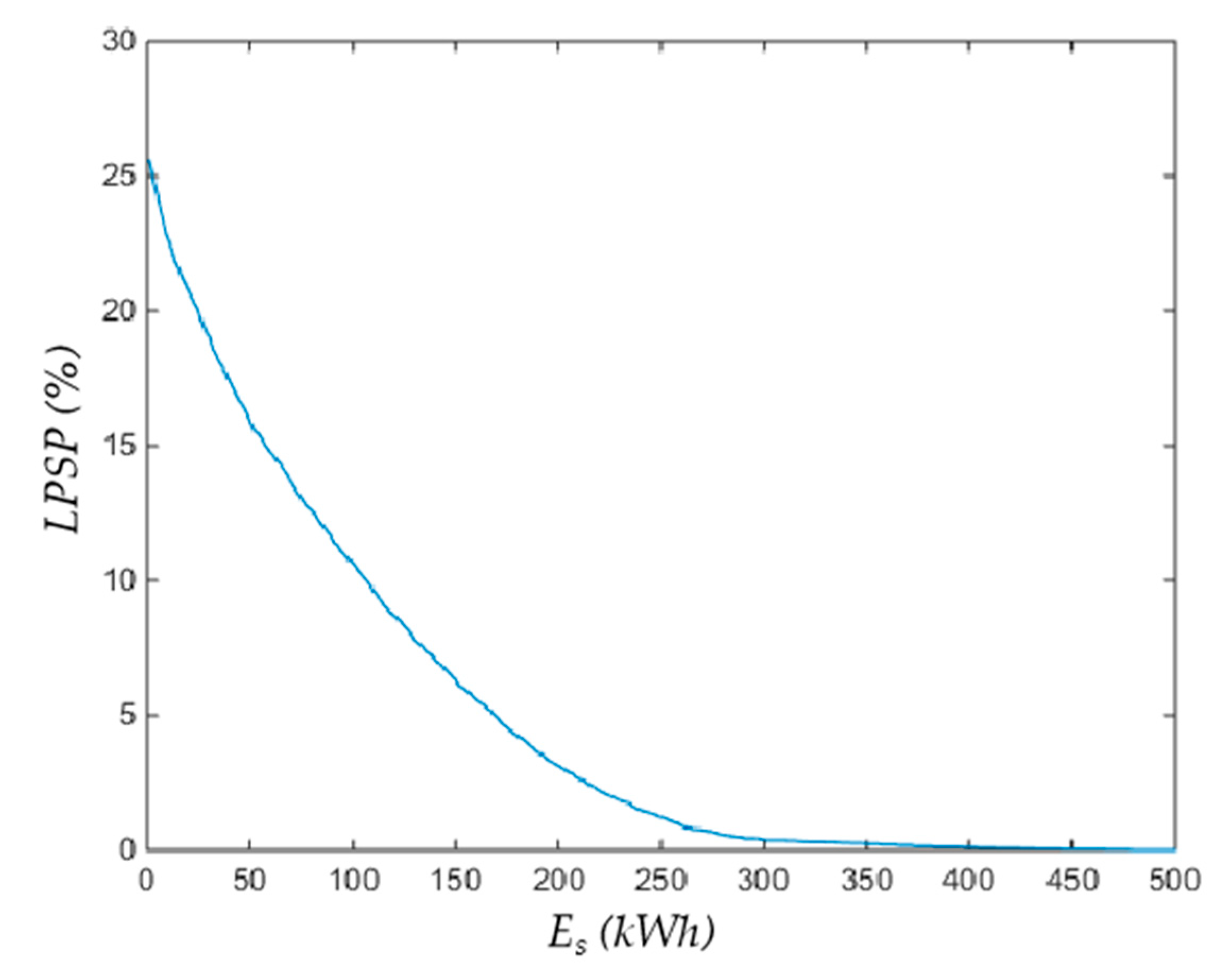
As discussed, the LPSP may not be a valid index to assess the power generation stability for a HWPS with the configuration determined by the probabilistic models. Given the temporal wind speed and solar irradiance data, the probability for power shortages could be calculated, but the possibility for power deficits in the future is unknown. The probabilistic approach proposed in the present study faces the future, and the expected power deficit duration is therefore of concern. In addition, the LPSP is related to the battery capacity of E_s in a nonlinear way. More specifically, the LPSP decreases exponentially with the increasing E_s, as shown in Figure 10 for a typical configuration of HWPS. Consequently, a small variation in the E_s could bring significant changes in the LPSP. In other words, the deviations and variations shown in Table 7 and Table 8 may not be the evidence of the shortcomings of the probabilistic approach to assess the power generation but an indicator of the ill-defined LPSP.

As indicated by in the calculation of LPSPs in the optimization and in the sensitivity analysis, the LPSP should be connected with the localized sea condition. In a more stable environment, the LPSP of 1% means an unnecessarily long expected power deficit duration. In other words, the LPSP should be interpreted as the localized power deficit duration, and the LPSP of 1% means a different duration at a different location. Consequently, the criterion of 1% applied universally across the South China Sea could be problematic, as the localized sea condition is not taken into consideration.

5. Conclusions

Among the renewable energy forms currently available in the market, the wind energy and solar energy are the two most feasible forms. Since the wind and solar power generation modules in a HWPS could share the same platform for the offshore sites, the LCOE of the energy generated from an offshore HWPS could be reduced compared to offshore wind farms.

The present study proposes an innovative approach to optimize the configuration of a HWPS when the LCOE is used as the objective and the stability of the power generation is used as the constraint. More specifically, while the previous studies concerning the optimization of the HWPS conventionally employed historical temporal data, the present study suggests using probabilistic models in estimating the power generated from the HWPS. In addition, the present study proposes a model of a battery-level coefficient, based on which the battery capacity can be probabilistically estimated, given the expected power shortage in a given continuous duration. When the model estimating the power generated from a HWPS with a specific configuration is combined with the widely used cost model, the optimization employing GA is discussed. In the optimization, the installed capacities of the wind turbines and PV arrays and the load are all taken as independent variables.

The configurations of the HWPSs installed at four potential sites in the South China Sea are optimized using the proposed probabilistic approach. In order to verify the proposed method, the LPSP values correspond with the potential HWPS sites where the optimal configurations are obtained from the proposed probabilistic method. The verification reveals that the specifications of the duration to calculate the expected power shortage could have significant impacts on the estimates of power generations. Consequently, the present study contains a sensitivity analysis concerning the continuous power deficit days. The optimization and sensitivity analyses both indicate that the well-established LPSP criterion of 1% should not be applied universally across the South China Sea. In fact, the LPSP should be interpreted, when facing the possibility, as the localized expected power deficit duration. In the areas with more stable winds and solar resources, the LPSP criterion can be relaxed when only the power deficit duration is concerned.