An Online Energy-Saving Driving Strategy for Metro Train Operation Based on the Model Predictive Control of Switched-Mode Dynamical Systems

Abstract

With the rapid development of urban rail transit systems and the consequent sharp increase of energy consumption, the energy-saving train operation problem has been attracting much attention. Extensive studies have been devoted to optimal control of a single metro train in an inter-station run to minimize the energy consumption. However, most of the existing work focuses on offline optimization of the energy-saving driving strategy, which still needs to be tracked in real train operation. In order to attain better performance in the presence of disturbances, this paper studies the online optimization problem of the energy-saving driving strategy for a single metro train, by employing the model predictive control (MPC) approach. Firstly, a switched-mode dynamical system model is introduced to describe the dynamics of a metro train. Based on this model, an MPC-based online optimization problem is formulated for obtaining the optimal mode switching times with minimal energy consumption for a single train in an inter-station run. Then we propose an algorithm to solve the constrained optimization problem at each time step by utilizing the exterior point penalty function method. The proposed online optimal train control algorithm which determines the mode switching times can not only improve the computational efficiency but also enhances the robustness to disturbances in real scenarios. Finally, the effectiveness and advantages of this online optimal train control algorithm are illustrated through case studies of a single train in an inter-station run.

1. Introduction

1.1. Background and Motivation

Urban rail transit, which can effectively alleviate traffic pressure in large modern cities, is widely recognized as an attractive mode of transportation due to its features of large capacity, high speed, safety, punctuality and energy-efficiency [1]. Many large cities in the world are committed to developing and expanding their metro train projects. As of 2016, the global light rail market value is estimated to be $180.78 billion, which is expected to increase 2.3% by 2020. With the expansion of the metro line scale and the quick growth of passenger traffic demand, the total energy consumption of train operations is increasing rapidly. Therefore, energy-efficient train operation for urban rail transit, which needs to reduce the energy consumption while ensuring safety and punctuality, is becoming an urgent problem, and researchers have been continually striving to address the energy-efficient train operation problem.

So far, extensive studies have been devoted to searching for the optimal driving strategy, which is considered to be a commonly used, effective way to reduce the energy consumption of metro train operation [2]. Most of the existing studies only focus on the offline optimization of the driving strategy, which will be taken as the reference trajectory by the automatic train operation (ATO) system for ensuring the train tracks the reference trajectory. Due to the fact that offline optimized trajectory does not consider the disturbance factors encountered in the actual operation, it is hard to ensure the optimality of online operation. In addition, the complex operation environment and uncertain operational delays can deteriorate the tracking accuracy. Online adjustment of the reference trajectory is particularly urgent because it can quickly respond to various changes during a train’s operation to enhance intelligence. An alternative solution is converting it to a conventional optimization problem by formulating the problem in the discrete domain and solving it online with a numerical method [3]. Therefore, it is of greater significance to address the online optimization problem of the driving strategy.

In the studies concerning the online trajectory optimization, the speed or force during the whole operation segment is taken as the optimization variable. Although high dimensions of the optimization variable can increase the degree of freedom, that will degrade the computational efficiency. According to the existing studies, the optimal train control strategy usually follows the sequential operation modes: maximum traction (MT), speed holding (SH), coasting (CS) and maximum braking (MB), in which the control of each mode is known. In this regard, it is practically efficient to optimize the mode switching times instead of the speed/force trajectory by modeling the train as a switched-mode dynamical system. In this paper, we will address the online optimization of energy-saving driving strategy with switching times as the optimization variables, so as to improve the computation efficiency and the robustness to disturbances.

1.2. Literature Review

Research on optimal driving strategy is actually done to solve the typical optimal control problem. The first work on optimal train control was carried out by Ishikawa in 1968 [4], in which the Pontryagin maximum principle was used to find optimal driving strategy for trains. He gave a result that the optimal train control strategy on level tracks with constant speed limit follows the fixed mode sequence of MT–SH–CS–MB. Since then, there have been many outstanding works on optimal train control based on optimal control theory and solved by the Pontryagin maximum principle [5,6,7], the method of which belongs to the category of analytic method. More recently, Albrecht et al. [8,9] made a detailed summary on the problem of finding an optimal driving strategy on an undulating track with variable speed restrictions. By using Pontryagin maximum principle, they gave the necessary conditions on an optimal strategy and pointed out that an optimal strategy always exists. However, for more complex actual train operation conditions, e.g., local constraints of state variables, nonlinear resistance and variable grade profiles, the analytic method cannot work well. In contrast, the dynamic programming (DP) method can cope with these complex issues [10,11,12]. In [10], the optimal train control problem was reformulated into a multi-stage decision process, and the optimal control strategy was obtained directly through the numerical DP. Similarly, when the optimal train control problem is discretized by numerical methods, many mathematical programming techniques can be used to solve the optimal train control problem, such as linear programming [13] and nonlinear programming [14]. As long as the computational time is enough, a near-optimal solution can be obtained by these numerical methods. In recent years, with the rise of various evolutionary algorithms, many scholars tried to use genetic algorithm (GA) [15], and ant colony optimization (ACO) [16] to solve the optimal train control problem, in which the optimality and convergence of the solutions cannot be guaranteed. In addition, because the operation of the train under actual running environment is very complex, the train cannot know many situations in advance. As you cannot calculate all the possible cases offline, evolutionary algorithms have some drawbacks. Furthermore, detailed reviews of the classical single-train control problem can be found in [1,17,18].

It is worth noting that the studies mentioned above only focused on the offline optimization of the driving strategy. In order to acquire better performance in the presence of disturbances, scholars have been paying more attention to the online optimization problem of the driving strategy. Considering the uncertain disturbances on resistance coefficients and the possible delay time, Yan et al. [19] proposed a moving horizon train optimization approach for dynamic train trajectory planning problem, which can be solved by immune differential evolution algorithm. Yan et al. [20] presented a cooperative energy-efficient trajectory planning scheme for multiple high-speed train movements using distributed model predictive control, under which each train can get the optimal speed trajectory online. Xun et al. [21] discussed an online train speed profile optimization problem solved by sequential quadratic programming. He et al. [22] developed a shrinking horizon MPC algorithm combined with the Radau pseudo-spectral method to obtain the optimal speed-time trajectory online based on the real-time information. We can easily see that in all these studies, the online optimization variable is the speed or force during the whole operation segment, which is high dimensional, and it will bring heavy computation cost so as to hinder online implementation.

Motivated by the fact that the optimal train control strategy usually follows the fixed mode sequence of MT–SH–CS–MB, some researchers have introduced the switched-mode dynamical system to describe the dynamics of a metro train [23,24], in which the optimization variable is the gear angle. In [25], based on the switched-mode dynamical system, the optimal driving problem was converted to a nonlinear optimization problem, and an exterior point method was proposed to calculate the driving strategies, in which the optimization variables were switching gear sequence and switching locations. However, these results cannot be applied to online optimization of reference trajectories.

1.3. The Focus of This Study

From the perspective of reducing the optimization variable’s dimensions to improve the computation efficiency, we regard the train as a switched-mode dynamical system, and then convert the online optimal train control problem to finding the optimal mode switching times online. A general optimal control framework for such systems was established in [26], and an online algorithm to calculate the optimal mode-switching times in switched-mode dynamical systems was investigated in [27]. Nevertheless, the proposed algorithms cannot be directly applied to solving the optimal train control problem due to the process and terminal state constraints in train operation.

In this paper, we address the online optimization of energy-saving driving strategy based on MPC, in which the train model is an switched-mode dynamical system and the optimization variables are switching times. An online algorithm is then presented to calculate the optimal switching times.

The main contributions of this paper are summarized as follows:

• A switched-mode dynamical system is introduced to describe the dynamics of a metro train. By using the switching times as the optimization variables, the defect of high dimension of the optimization variable in [3,19,20,21,22,28] can be avoided such that the computation cost can be reduced.
• By employing MPC, an online algorithm is presented to obtain the optimal switching times at each sampling instant, which partially extends the offline optimization in [25] to online optimization, and can timely respond to disturbances during train operation.

The remainder of this paper is organized as follows. In Section 2, the basic optimal train control problem is described, along with train traffic model and energy consumption model. In Section 3, a switched-mode dynamical system model is presented to describe the dynamics of a metro train, and the MPC-based online optimization problem is formulated for obtaining energy-saving switching times. An algorithm to solve the proposed optimization problem is proposed in Section 4. Section 5 of this paper presents case studies for metro trains to demonstrate the effectiveness of the proposed algorithm. In Section 6, we conclude the whole paper.

To describe and understand the proposed method easily, we summarize the notation needed in our formulation in Appendix A.

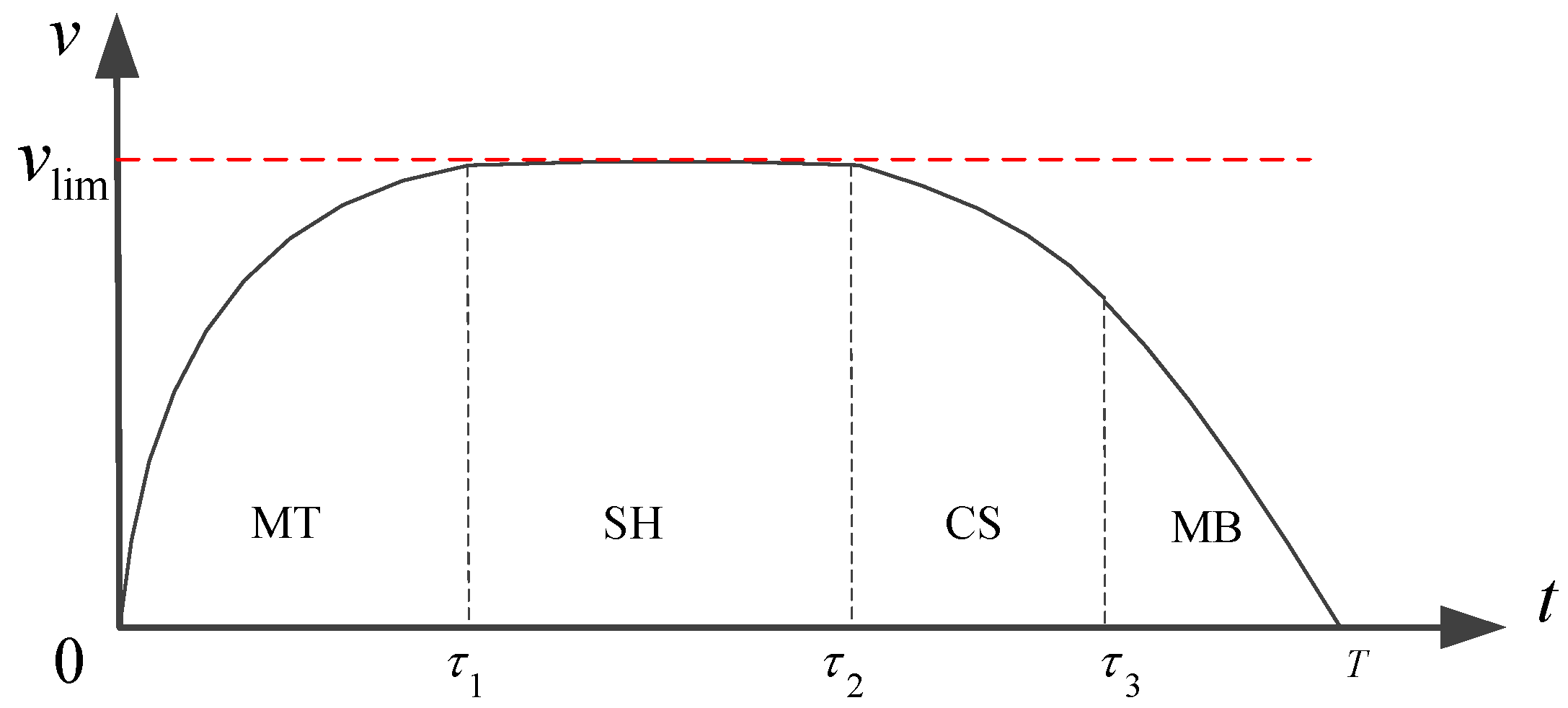
2. The Optimal Train Control Problem

In this section, the basic optimal train control problem is reviewed briefly, including the basic notation and the main modeling concepts which will be used later in this paper. The movement of a point-mass train with time as the independent variable is described as:

$$\frac{dp}{dt}=v$$

(1)

$$\frac{dv}{dt}=\frac{1}{M}(u-R(v)-G(p))$$

(2)

where $p=p(t)$ is the train position (m) and $v=v(t)$ is the train speed (m/s); M is the total mass of the train; $u=u(t)$ is the instantaneous force applied to the train; $R(v)$ is the resistance force which is usually approximated in terms of a quadratic function of v by equation as

$$R(v)=a_0+a_{1}v+a_2{v}^2$$

(3)

where the parameters $a_0$, $a_1$ and $a_2$ are the rolling resistance coefficient, the mechanical resistance coefficient and the external air resistance coefficient, respectively; $G(p)$ is the gradient resistance along the track; i.e.,

$$G(p)=Mgsin(arctan\theta (p))\approx Mg\theta (p)$$

(4)

with g being the gravitational acceleration, and $\theta (p)$ being the track gradient at location p. The speed of the running train is bounded as follow,

$$0\le v(t)\le v_{lim}$$

(5)

where $v_{lim}$ is the upper speed limit at location p. Considering the performance of train power system, the applied force should be limited within a proper range:

$$-B_{max}(v)\le u\le T_{max}(v)$$

(6)

According to the characteristics of electric trains, the effort of a tractive motor is divided into a “constant torque region” and a “constant power region” [29]. As shown in Figure 1, we suppose that maximum traction and maximum braking are piecewise linear functions with respect to speed, where $v^c$ is the critical speed at which the maximum tractive/braking force function switches from one piece to the other. The piece with speed lower than $v^c$ is called Regime 1 and the piece with speed higher than $v^c$ is called Regime 2. Suppose $v^c=v^a$ for $T_{max}$, and $v^c=v^b$ for $B_{max}$.

$$T_{max}(v)=\left\{\begin{array}{c}{\alpha }_{1}v+{\beta }_1,0\le v\le v_a\hfill \\ {\alpha }_{2}v+{\beta }_2,v>v_a\hfill \end{array}\right.,{\alpha }_1\le 0,{\alpha }_2\le 0,{\beta }_1\ge 0,{\beta }_2\ge 0$$

(7)

and

$$B_{max}(v)=\left\{\begin{array}{c}{\lambda }_{1}v+{\xi }_1,0\le v\le v_b\hfill \\ {\lambda }_{2}v+{\xi }_2,v>v_b\hfill \end{array}\right.,{\lambda }_1\le 0,{\lambda }_2\le 0,{\xi }_1\ge 0,{\xi }_2\ge 0$$

(8)

Consider the problem of driving a train as described by Equations (1) and (2) from one station to the next along a level track within a given allowable time T to minimize the energy consumption. Then, the optimal train control problem can be formally described as follows:

$$min\underset{0}{\overset{T}{\int }}max\{u(t),0\}v(t)dt$$

(9)

$$p(0)=0,p(T)=P,v(0)=0,v(T)=0$$

(10)

where P is the length between two adjacent stations. Given the train dynamics (1) and (2) with initial and terminal constraints (10), find a control law u such that the objective function (9) is minimized subject to the constraints.

3. Online Energy-Saving Driving Strategy Based on MPC of Switched-Mode Systems

In this section, the dynamic model of a metro train is established as a switched-mode dynamical system. Then, the MPC-based online optimization problem is formulated with mode-switching times as the optimization variables to minimize the energy consumption for a single train in an inter-station run.

3.1. Train Switched-Mode Dynamical Model

Firstly, a switched-mode dynamical system model is introduced to describe the characteristics of a metro train. It is commonly recognized that the energy-saving strategy on level tracks with constant speed limit for an individual train inter-station run under a given running time uses four modes of movement, namely, MT, SH, CS and MB in sequence (see Figure 2). Given a fixed time horizon $[0,T]$, let ${\tau }_i$, $i=1,2,3$ be a finite sequence of mode-switching time instants such that $0\le {\tau }_1\le {\tau }_2\le {\tau }_3\le T$. ${\tau }_1,{\tau }_2,{\tau }_3$ are the time instants to start SH, CS and MB respectively, as shown in Figure 2.

Considering the train running between two stations, its dynamic equation is:

$$\dot{x}=f(x,t),x={[p,v]}^T$$

(11)

$$f(x,t)=\left[\begin{array}{c}v\\ M^{-1}(u-R(v)-Mg\theta (p))\end{array}\right]$$

(12)

The variable $x(t)$ is the state of the system, and the force applied in each stage is given as follows:

$$u=\left\{\begin{array}{c}{T}_{max}\hfill \\ R(v)+Mg\theta (p)\hfill \\ 0\hfill \\ -B_{max}\hfill \end{array}\right.\begin{array}{c}\mathrm{MT}\\ \mathrm{SH}\\ \mathrm{CS}\\ \mathrm{MB}\end{array}$$

(13)

where $R(v)$ is a quadratic function of v given in Equation (3). Considering the train runs on level track, $Mg\theta (p)$ is equal to zero. Substituting Equation (13) into the speed dynamic (2), we have

$$\frac{dv}{dt}=\left\{\begin{array}{c}{M}^{-1}(T_{max}-R(v))\hfill \\ 0\hfill \\ -M^{-1}R(v)\hfill \\ -M^{-1}(B_{max}+R(v))\hfill \end{array}\right.\begin{array}{c}\mathrm{MT}\\ \mathrm{SH}\\ \mathrm{CS}\\ \mathrm{MB}\end{array}$$

(14)

Thus, the switched-mode dynamical system concerned can be written as

$$\dot{x}=\left\{\begin{array}{cc}{f}_1(x)={[v,M^{-1}(T_{max}(v)-R(v))]}^T,\hfill & t\in [0,{\tau }_1)\\ f_2(x)={[v,0]}^T,\hfill & t\in [{\tau }_1,{\tau }_2)\\ f_3(x)={[v,-M^{-1}R(v)]}^T,\hfill & t\in [{\tau }_2,{\tau }_3)\\ f_4(x)={[v,-M^{-1}(B_{max}(v)+R(v))]}^T,\hfill & t\in [{\tau }_3,T)\end{array}\right.$$

(15)

with a given initial condition $x_0:=x(0)$. The functions $f_i$, $i=1,2,3,4$ are called the modal functions, and the times ${\tau }_i$, $i=1,2,3$ are called the switching times.

3.2. Optimization of Switching Times via MPC

Considering the train switched-mode dynamical system (15), a train runs from one station to the next along a level track within a given time T. Let us denote the vector of switching times by $\overline{\tau }:={[{\tau }_1,{\tau }_2,{\tau }_3]}^T$. Define the feasible set as $\Lambda =\{\overline{\tau }={[{\tau }_1,{\tau }_2,{\tau }_3]}^T\}$ subject to the constraints:

$$0\le {\tau }_1\le {\tau }_2\le {\tau }_3\le T$$

(16)

The sequence of modes (MT, SH, CS and MB) is fixed, which is commonly recognized as the energy-saving sequence for an individual train in an inter-station run under a given run-time. Then we have the power function for train at time $t\in [0,T)$ denoted by $L(x)$, which is a piecewise function, i.e.,

$$L(x)=\left\{\begin{array}{cc}{L}_1(x)=T_{max}(v)v,\hfill & t\in [0,{\tau }_1)\\ L_2(x)=R(v)v,\hfill & t\in [{\tau }_1,{\tau }_2)\\ L_3(x)=0,\hfill & t\in [{\tau }_2,{\tau }_3)\\ L_4(x)=-\epsilon B_{max}(v)v,\hfill & t\in [{\tau }_3,T)\end{array}\right.$$

(17)

with $\epsilon \in (0,1)$ representing the efficiency factor in converting kinetic to electrical energy during the regenerative braking.

Then, we formulate the online optimization problem with respect to switching times. Assume the metro train measures its current state at each sampling instant $t_k=k\Delta t$ with $k=0,1,2\dots$ and $\Delta t$ being the sampling period, and then solves an MPC-based optimization problem to determine its switching times at the same time. Define the cost-to-go function for train at time $t_k\in [t,T)$ as

$$J(x(t|t_k),\overline{\tau }(t_k))={\int }_{t_k}^{T}L(x(t|t_k))dt$$

(18)

where $x(t|t_k)$, $t\in [t_k,T]$ is the future state trajectory of the train predicted at $t_k$ with respect to $\overline{\tau }(t_k)$. The $\overline{\tau }(t_k)={[{\tau }_1(t_k),{\tau }_2(t_k),{\tau }_3(t_k)]}^T$ is the vector of the switching times at time $t_k$. We define the integer $i(t_k,\overline{\tau }(t_k))$ as the index $(n)$ of the last switching time that has taken place before or at time $t_k$, which is given as below:

$$i(t_k,\overline{\tau }(t_k))=max\{n=0,1,2,3|{\tau }_n(t_k)\le t_k\},$$

Obviously, ${{\tau }_i}_{(t_k,\overline{\tau }(t_k))}\le t_k\le {{\tau }_i}_{(t_k,\overline{\tau }(t_k))+1}$. The cost-to-go function (18) is not affected by the switching time that has taken place prior to time $t_k$ and is only related to the future switching times ${{\tau }_n}_{(t_k,\overline{\tau }(t_k))}$, $n=i(t_k,\overline{\tau }(t_k))+1,\cdots ,3$. It should be noted that the actual variable $\overline{\tau }(t_k)$ is only a sub-vector of $\overline{\tau }$ including the future switching times. Nonetheless, we use $\overline{\tau }(t_k)$ in (18) for notational brevity. When $t_k\in [0,T)$, the train solves the following optimization problem:

$${\overline{\tau }}^{*}(t_k)=arg\underset{\overline{\tau }(t_k)}{min}J(x(t|t_k),\overline{\tau }(t_k))$$

(19)

s.t.

$$\left\{\begin{array}{c}x(t_k|t_k)=x(t_k)\hfill \\ \dot{x}(t|t_k)=f(x(t|t_k)),t\in [t_k,T)\hfill \\ x(T|t_k)={[P,0]}^T\hfill \\ 0\le v(t|t_k)\le v_{lim},t\in [t_k,T)\hfill \\ 0\le {\tau }_1(t_k)\le {\tau }_2(t_k)\le {\tau }_3(t_k)\le T\hfill \end{array}\right.$$

With $\overline{\tau }(t_k)$ being the optimal control scheme ${\overline{\tau }}^{*}(t_k)$, the corresponding predicted state is also optimal and denoted by $x^{*}(t|t_k)$ for $t\in [t_k,T)$.

The online control of the train is realized through the following process. At each sampling instant $t_k$, the current state information can be obtained by on-board equipment directly. By solving optimization problem (19), we can obtain the optimal switching times ${\overline{\tau }}^{*}(t_k)$. As long as the current time $t_k<{{\tau }_i}_{(t_k,{\overline{\tau }}^{*}(t_k))+1}$, the train continues to operate in the current mode. When the current time $t_k\ge {{\tau }_i}_{(t_k,{\overline{\tau }}^{*}(t_k))+1}$, the train switches to the next mode.

4. Solution Algorithm Development

In this section, we present an algorithm to solve the optimization problem (19). Concerning the switching time optimization problem, a number of algorithms have been developed in [27,30]. However, these algorithms cannot be directly applied to solving the optimization problem (19) due to the existence of a terminal state constraint.

As it is difficult to select the initial value which satisfies the terminal state constraints, the exterior point penalty function method is a reasonable solution.

In addition, the optimal solution should satisfy constraint $\overline{\tau }\in \Lambda$. One should observe that this constraint can be viewed as a series of linear inequality constraints, and the projection method can be applied. The projection can be easily and quickly obtained by using the algorithm given in reference [31]. Using this method, we can ignore the constraint, unless the constraint is active and the iteration point is on the boundary of the constraint, in which case the projection of the descent direction onto the feasible set should be used as the feasible direction.

Combined with the online optimization algorithm given in reference [27], we proposed an online algorithm based on the penalty function method.

Firstly, we construct a new cost function as:

$$J(t_k,x(t|t_k),\overline{\tau }(t_k),\gamma )={\int }_{t_k}^{T}L(x(t|t_k)dt+\gamma {(p(t_k)+{\int }_{t_k}^{T}v(t|t_k)dt-P)}^2+\gamma v{(T|t_k)}^2$$

(20)

Here, $\gamma$ is a penalty factor; the first penalty item is to satisfy the constraint of running distance at the terminal time step, and the second penalty item is to satisfy the zero speed constraint when the train arrives at the station.

Then, the detailed algorithm to solve the optimization problem (19) is described as follows.

The Algorithm 1 mainly includes three loops. The outermost loop is to control the solving of the optimization problem at each sampling time step k to get the optimal switching times until the train stops at the next station. The loop in the middle layer is to control the iterative updating of the penalty factor $\gamma$, where the minimization of (20) with each value of $\gamma$ is solved until the total value of penalty terms decreases below a pre-set threshold $\varsigma$. The innermost loop is used to control the iterative updating of the switching times until the gradient of the current cost function decreases below a pre-set threshold $\vartheta$. Note that at the beginning of the Algorithm 1, the related parameters $\overline{\tau }(0)$, ${\gamma }_{PR}$, $\rho$, $\varsigma$ and $\vartheta$ need to be initialized. At each time step k, the train needs to collect the current state information, including speed and position, and then calculate the optimal switching time following the iterative updating of ${\gamma }_j$ and ${\overline{\tau }}_q^j$ until both judging conditions with respect to $\varsigma$ and $\vartheta$ are satisfied.

Algorithm 1 Online computation of ${\overline{\tau }}^{*}(t_k)$.

Require: track length P, running time T, current state $x(t_k)$

Ensure:${\overline{\tau }}^{*}(t_k)$,${\gamma }_{PR}$

1: Set $k=0$, choose an initial point $\overline{\tau }(0)\in \Lambda$, set ${\overline{\tau }}^{*}(t_{-1})=\overline{\tau }(0)$.   2: Set $j=1$, initialize ${\gamma }_{PR}$, $\rho >1$, $\varsigma$, $\vartheta$, ${\gamma }_1={\gamma }_{PR}$.   3: Set $q=1$, initialize ${\overline{\tau }}_q^j(t_k)={\overline{\tau }}^{*}(t_{k-1})$.   4: Construct the cost-to-go function $J(t_k,x(t|t_k),{\overline{\tau }}_q^j(t_k),{\gamma }_j)$.   5: Define $\nabla g({\overline{\tau }}_q^j(t_k))=\frac{\partial J}{\partial \overline{\tau }(t_k)}(t_k,x(t|t_k),{\overline{\tau }}_q^j(t_k),{\gamma }_j)$.   6: if $\left|\right|\nabla g({\overline{\tau }}_q^{{}_j}(t_k))\left|\right|<\vartheta$, go to step 8, else go to step 7.   7: Compute ${\tilde{h}}_q^j(t_k)$ as the projection of $-H_q^j{(t_k)}^{-1}\frac{\partial J}{\partial \overline{\tau }(t_k)}(t_k,x(t|t_k),{\overline{\tau }}_q^j(t_k),{\gamma }_j)$ onto the feasible set $\Lambda$ at $\overline{\tau }(t_k)$, where $H_q^j(t_k)=\frac{{\partial }^{2}J}{{\partial }^2\overline{\tau }(t_k)}(t_k,x(t|t_k),{\overline{\tau }}_q^j(t_k),{\gamma }_j)$. Let ${\overline{\tau }}_{q+1}^j(t_k)={\overline{\tau }}_q^j(t_k)+{\kappa }_q^j(t_k){\tilde{h}}_q^j(t_k)$ with ${\kappa }_q^j(t_k):=max\{d\le 1|{\overline{\tau }}_q^j(t_k)+d{\tilde{h}}_q^j(t_k)isfeasible\}$. Set $q=q+1$ and go to step 4.   8: If ${\gamma }_j({(p(t_k)+{\int }_0^{T}v(t|t_k)dt-P)}^2+v{(T|t_k)}^2)<\varsigma$, go to step 9. Otherwise, set $j=j+1,{\gamma }_j=\rho {\gamma }_{j-1}$, and go to step 3.   9: Return:${\overline{\tau }}^{*}(t_k)={\overline{\tau }}_q^j(t_k)$, ${\gamma }_{PR}={\gamma }_j$. 10: Set $k=k+1$, and go to step 2.

5. Case Studies

In this section, in order to verify the efficiency of the proposed online optimal switching time-based driving strategy, the proposed Algorithm 1 was applied to a metro train to implement the numerical experiments. The scenario of an inter-station run for a single train is shown in Figure 3, which indicates that the operation mode sequence is MT–SH–CS–MB and an inter-station run with the fixed operation mode sequence has many different driving trajectories with different switching times. Our objective was to find the one with minimum energy consumption. In Section 5.1, the main train parameters are given. In Section 5.2, case studies of two different inter-station runs with fixed running times are presented. In Section 5.3, we analyze the changes of switching times and energy consumption with different running times. In Section 5.4, the train’s operation with a disturbance is analyzed. All computations throughout the following numerical experiments were performed by MATLAB R2016b on a PC (3.30 GHz processor speed and 8-GB RAM) with Microsoft Windows 7 platform.

5.1. Parameter Setting

Here, the online optimal switching time driving strategy for the metro train DKZ32 is studied, which is used in Beijing Yizhuang metro line of China. Each train consists of three motor cars and three trailer cars; the train is powered by DC 750 V supply via third-rail. The main train parameters are listed as follows.

• $M=2.78\times {10}^5$ kg.
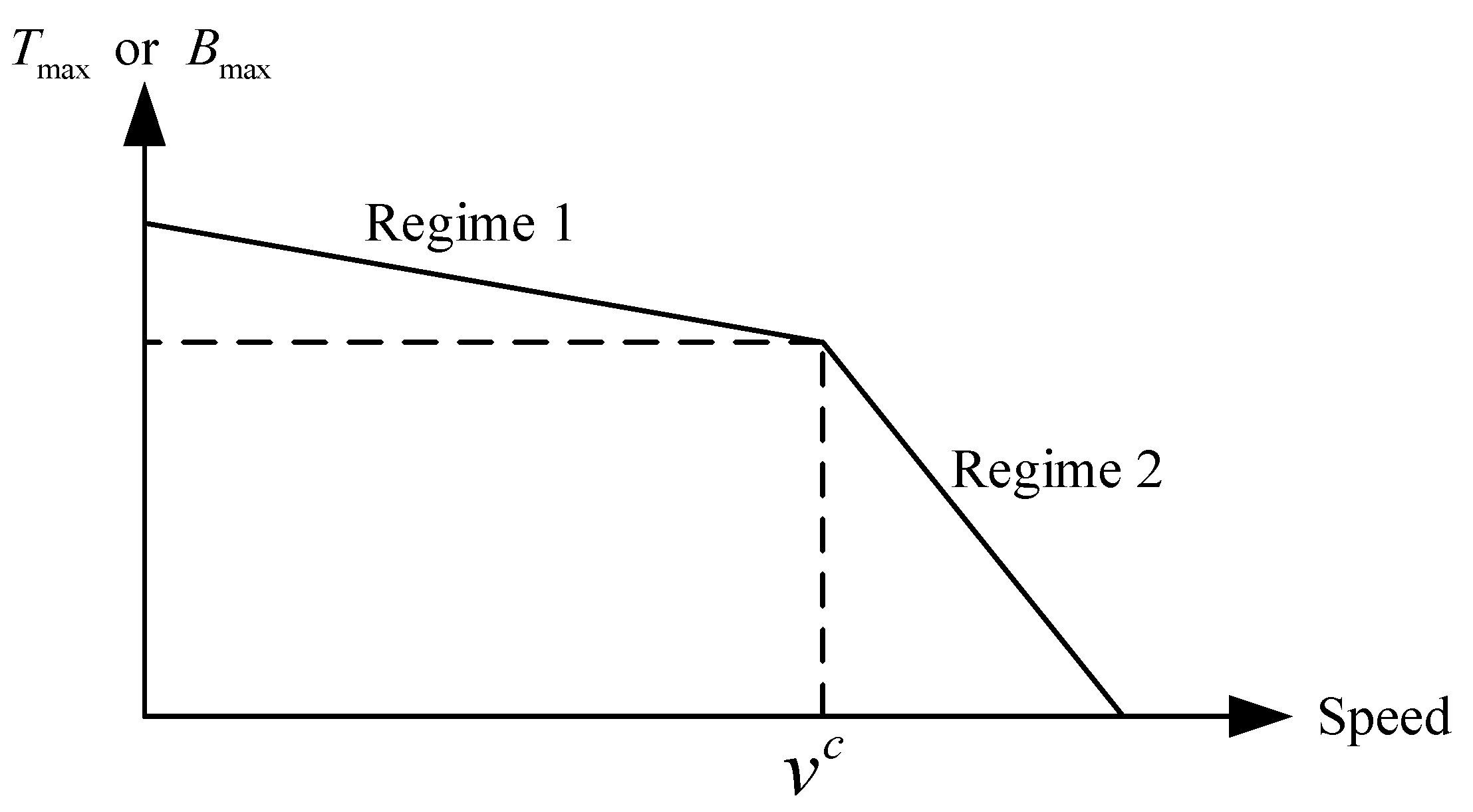
• The maximum traction force is given as follows.

  $$T_{\max }=\left\{\begin{array}{cc}310\mathrm{kN}\hfill & v\le 10\mathrm{m}/\mathrm{s}\hfill \\ 310-18(v-10)\mathrm{kN}\hfill & 10<v\le 22.2\mathrm{m}/\mathrm{s}.\hfill \end{array}\right.$$
• The maximum electrical braking force is calculated by:

  $$B_{\max }=\left\{\begin{array}{cc}260\mathrm{kN}\hfill & v\le 15\mathrm{m}/\mathrm{s}\hfill \\ 260-18(v-15)\mathrm{kN}\hfill & v>15\mathrm{m}/\mathrm{s}.\hfill \end{array}\right.$$
• The running resistance can be calculated by:

  $$R(v)=2.2294\times {10}^{-3}{v}^2+3.9476\mathrm{kN}.$$
• The efficiency factor $\epsilon =0.4$.

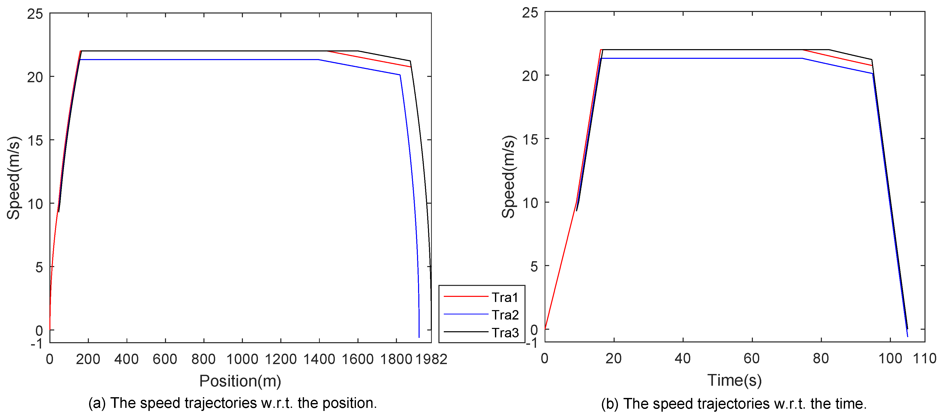
5.2. Inter-Station Run with Fixed Running Time

In this subsection, we chose two different intervals of Beijing Yizhuang metro line as examples, the line parameters of which are shown in

Table 1. The line parameters.

Inter-Station	P (m)	T (s)	${\mathit{v}}_{\mathbf{lim}}$ (m/s)
Jiugong–Yizhuangqiao	1982	130	22.2
Yizhuangqiao-Wenhuayuan	993	90	22.2

.

The optimal speed trajectories obtained by the Algorithm 1 for Jiugong–Yizhuangqiao and Yizhuangqiao–Wenhuayuan intervals are shown in Figure 4 and Figure 5 respectively, where (a) corresponds to the speed trajectories with respect to the position and (b) corresponds to those with respect to the time. The optimal switching times and the corresponding energy consumption values for Jiugong–Yizhuangqiao and Yizhuangqiao–Wenhuayuan intervals are given in

Table 2. The optimal $\overline{\tau }$ and energy consumption.

Inter-Station	${\mathit{\tau }}_{\mathbf{1}}$	${\mathit{\tau }}_{\mathbf{2}}$	${\mathit{\tau }}_{\mathbf{3}}$	$\mathit{E} (\mathbf{kw}·\mathbf{h})$
Jiugong–Yizhuangqiao	14.4	14.4	122.9	11.27
Yizhuangqiao–Wenhuayuan	11	11	84.5	7.4

.

5.3. Analysis of Different Running Times

In this subsection, we analyze the changes of switching times and energy consumption with different running times. We take the interval from Jiugong Station to Yizhuangqiao Station of Beijing Yizhuang metro line as an example. We take 105, 110, 115 and 120 s as the given running times, respectively, and let the train operate following the Algorithm 1. Then the optimal speed trajectories with these different running times are shown in Figure 6, where (a) corresponds to the speed trajectories with respect to the position and (b) corresponds to those with respect to the time. The switching times and energy consumption with different running times are shown in

Table 3. The optimal $\overline{\tau }$ values and energy consumption of different running times T.

T (s)	105	110	115	120
${\tau }_1$	16.1	16.1	16.1	15.4
${\tau }_2$	74.5	35.6	16.1	15.4
${\tau }_3$	94.8	101	106.6	112.1
$E (\mathrm{kw}·\mathrm{h})$	19.1	16.1	14.5	13.2

. We can easily observe that with the increase of running time, the proportion of coasting in the optimal speed trajectories is increased, and the energy consumption is reduced.

5.4. Analysis with Disturbance

In this case, we simulate the train operation with a disturbance under the Algorithm 1. The line parameters are the same as those in Section 5.3, and the given running time is 105 s. We assume that the train runs to a certain point under disturbance at $t_k=9.1$ s with $p(t_k)=45$ m and $v(t_k)=9.3$ m/s. The pre-optimized trajectory without disturbance is shown by Tra1 in Figure 6, in which the train speed at $t_k=9.1$ s should be 10 m/s. If the disturbance is exerted, the train will eventually fail to meet the terminal constraints under the pre-optimized switching time, which is illustrated by Tra2 in Figure 6. The trajectory Tra3 in Figure 7 represents the updated result under the Algorithm 1. As the train fails to reach the predetermined speed under disturbance, the cruising time is increased after the train reaches the speed limit. Under the updated switching times, the train will operate with the energy optimization manner and meet the terminal constraints simultaneously.

5.5. Discussion

Firstly, through the above case studies, the feasibility of the proposed algorithm is verified, and the results obtained are consistent with the previous conclusions on optimal train control. Secondly, because the number of decision variables in the optimal train control problem is only three, the scale of the optimization problem is greatly reduced so as to improve the computation efficiency, which makes online computation possible. In addition, when the train deviates from the original optimal trajectory due to disturbances, the Algorithm 1 can recalculate the optimal strategy of the remaining journey according to the latest state of the train, so we can say the online driving strategy proposed in this paper is robust to disturbances.

6. Conclusions

This paper has studied the online energy-saving driving strategy for a single metro train. A switched-mode dynamical system model has been established with the consideration of regenerative braking energy, which can accurately describe the metro train operation mode and punctuality constraint. According to the previous conclusions on optimal train control, the optimal train operation strategy has a fixed operation sequence(MT–SH–CS–MB). Therefore, the switching system model established in this paper has four modes, and the optimal control of each mode is known, which can be regarded as the speed feedback control. Therefore, as long as the current state of the train is obtained, the optimal control under the current mode can be obtained. The critical problem is to determine the optimal mode switching times. On this basis, an online optimization problem with switching times as the optimization variables has been formulated to minimize the energy consumption by employing the MPC approach, and an online algorithm to solve the optimization problem has also been introduced by utilizing the exterior point penalty function method. The proposed online algorithm with the switching times as the optimization variables cannot only respond in a timely way to disturbances during train operation, but also improve the computational efficiency which can realize online real-time application. Case studies have been presented to verify the feasibility and advantages of the proposed algorithm. We may further consider the online multi-train energy-saving operation based on the switched-mode dynamical systems as our future work.

References

1. Yang, X.; Li, X.; Ning, B.; Tang, T. A Survey on Energy-Efficient Train Operation for Urban Rail Transit. IEEE Trans. Intell. Transp. Syst. 2016, 17, 2–13. [Google Scholar] [CrossRef]
2. González-Gil, A.; Palacin, R.; Batty, P.; Powell, J.P. A systems approach to reduce urban rail energy consumption. Energy Convers. Manag. 2014, 80, 509–524. [Google Scholar] [CrossRef] [Green Version]
3. Yazhemsky, D.; Rashid, M.; Sirouspour, S. An On-Line Optimal Controller for a Commuter Train. IEEE Trans. Intell. Transp. Syst. 2019, 20, 1112–1125. [Google Scholar] [CrossRef]
4. Ishikawa, K. Application of optimization theory for bounded state variable problems to the operation of trains. Bull. Jpn. Soc. Mech. Eng. 1968, 11, 857–865. [Google Scholar] [CrossRef]
5. Milroy, I.P. Aspects of Automatic Train Control. Ph.D. Thesis, Loughborough University, Loughborough, UK, 1980. [Google Scholar]
6. Howlett, P. Optimal strategies for the control of a train. Automatica 1996, 32, 519–532. [Google Scholar] [CrossRef]
7. Liu, R.R.; Golovitcher, I.M. Energy-efficient operation of rail vehicles. Transp. Res. Part A Policy Pract. 2003, 37, 917–932. [Google Scholar] [CrossRef]
8. Albrecht, A.; Howlett, P.; Pudney, P.; Xuan, V.; Zhou, P. The key principles of optimal train control-Part 1: Formulation of the model, strategies of optimal type, evolutionary lines, location of optimal switching points. Transp. Res. B Methodol. 2016, 94, 482–508. [Google Scholar] [CrossRef]
9. Albrecht, A.; Howlett, P.; Pudney, P.; Xuan, V.; Zhou, P. The key principles of optimal train control-Part 2: Existence of an optimal strategy, the local energy minimization principle, uniqueness, computational techniques. Transp. Res. B Methodol. 2015, 94, 509–538. [Google Scholar] [CrossRef]
10. Ko, H.; Koseki, T.; Miyatake, M. Application of dynamic programming to the optimization of the running profile of a train. Comput. Railw. 2004, 45, 8. [Google Scholar]
11. Lu, S.; Hillmansen, S.; Ho, T.K.; Roberts, C. Single-Train Trajectory Optimization. IEEE Trans. Intell. Transp. Syst. 2013, 14, 743–750. [Google Scholar] [CrossRef]
12. Haahr, J.T.; Pisinger, D.; Sabbaghian, M. A dynamic programming approach for optimizing train speed profiles with speed restrictions and passage points. Transp. Res. Part B Methodol. 2017, 99, 167–182. [Google Scholar] [CrossRef] [Green Version]
13. Wang, Y.; de Schutter, B.; van den Boom, T.J.; Ning, B. Optimal trajectory planning for trains—A pseudospectral method and a mixed integer linear programming approach. Transp. Res. Part C Emerg. Technol. 2013, 29, 97–114. [Google Scholar] [CrossRef]
14. Ye, H.; Liu, R. Nonlinear programming methods based on closed-form expressions for optimal train control. Transp. Res. Part C Emerg. Technol. 2017, 82, 102–123. [Google Scholar] [CrossRef] [Green Version]
15. Youneng, H.; Xiao, M.; Shuai, S.; Tao, T. Optimization of Train Operation in Multiple Interstations with Multi-Population Genetic Algorithm. Energies 2015, 8, 14311–14329. [Google Scholar]
16. Ke, B.; Chen, M.; Lin, C. Block-Layout Design Using MAX–MIN Ant System for Saving Energy on Mass Rapid Transit Systems. IEEE Trans. Intell. Transp. Syst. 2009, 10, 226–235. [Google Scholar]
17. Scheepmaker, G.M.; Goverde, R.M.; Kroon, L.G. Review of energy-efficient train control and timetabling. Eur. J. Oper. Res. 2017, 257, 355–376. [Google Scholar] [CrossRef] [Green Version]
18. Yin, J.; Tao, T.; Yang, L.; Jing, X.; Gao, Z. Research and development of automatic train operation for railway transportation systems: A survey. Transp. Res. C Emerg. Technol. 2017, 85, 548–572. [Google Scholar] [CrossRef]
19. Yan, X.; Cai, B.; Ning, B.; ShangGuan, W. Moving Horizon Optimization of Dynamic Trajectory Planning for High-Speed Train Operation. IEEE Trans. Intell. Transp. Syst. 2016, 17, 1258–1270. [Google Scholar] [CrossRef]
20. Yan, X.; Cai, B.; Ning, B.; Wei, S.G. Online distributed cooperative model predictive control of energy-saving trajectory planning for multiple high-speed train movements. Transp. Res. Part C Emerg. Technol. 2016, 69, 60–78. [Google Scholar] [CrossRef]
21. Liu, X.; Xun, J.; Ning, B.; Liu, T.; Xiao, X. Moving Horizon Optimization of Train Speed Profile Based on Sequential Quadratic Programming. In Proceedings of the 2018 International Conference on Intelligent Rail Transportation (ICIRT), Singapore, 12–14 December 2018; pp. 1–5. [Google Scholar]
22. He, D.; Zhou, L.; Sun, Z. Energy-efficient receding horizon trajectory planning of high-speed trains using real-time traffic information. Control Theory Technol. 2020, 18, 204–216. [Google Scholar] [CrossRef]
23. Le, Y.W.; Beydoun, A.; Cook, J.; Jing, S.; Kolmanovsky, I. Optimal Hybrid Control With Applications to Automotive Powertrain Systems; Springer: Berlin/Heidelberg, Germany, 1997. [Google Scholar]
24. Beydoun, A.; Le, Y.W.; Jing, S.; Sivashanka, S. Hybrid Control of Automotive Powertrain Systems: A Case Study; Springer: Berlin/Heidelberg, Germany, 1998. [Google Scholar]
25. Liang, L.; Wei, D.; Ji, Y.; Zhang, Z.; Lang, T. Minimal-Energy Driving Strategy for High-Speed Electric Train with Hybrid System Model. IEEE Trans. Intell. Transp. Syst. 2013, 14, 1642–1653. [Google Scholar]
26. Branicky, M.S.; Borkar, V.S.; Mitter, S.K. A unified framework for hybrid control: Model and optimal control theory. IEEE Trans. Autom. Control 1998, 43, 31–45. [Google Scholar] [CrossRef] [Green Version]
27. Ding, X.C.; Wardi, Y.; Egerstedt, M. On-Line Optimization of Switched-Mode Dynamical Systems. IEEE Trans. Autom. Control. 2007, 54, 2266–2271. [Google Scholar] [CrossRef]
28. Li, L.; Dong, W.; Ji, Y.; Zhang, Z. A minimal-energy driving strategy for high-speed electric train. J. Control Theory Appl. 2012, 10, 280–286. [Google Scholar] [CrossRef]
29. Lu, S.; Hillmansen, S.; Roberts, C. A power-management strategy for multiple-unit railroad vehicles. IEEE Trans. Veh. Technol. 2010, 60, 406–420. [Google Scholar] [CrossRef]
30. Azuma, S.I.; Egerstedt, M.; Wardi, Y. Output-based optimal timing control of switched systems. In Proceedings of the International Workshop on Hybrid Systems: Computation and Control, LNCS, Santa Barbara, CA, USA, 29–31 March 2006; Volume 3927, pp. 64–78. [Google Scholar]
31. Axelsson, H. Optimal Control of Switched Autonomous Systems: Theory, Algorithms, and Robotic Applications. Ph.D. Thesis, Georgia Institute of Technology, Atlanta, GA, USA, 2006. [Google Scholar]
Figure 1. Example of the maximum tractive or maximum braking force.
Energies 13 04933 g001
Figure 2. Optimal driving regimes for energy-efficient driving on a level track as a function of time with switching points.
Energies 13 04933 g002
Figure 3. The scenario of an inter-station run for a single train.
Energies 13 04933 g003
Figure 4. Optimal speed trajectory of Jiugong–Yizhuangqiao. (a) The speed trajectory w.r.t. the position; (b) The speed trajectory w.r.t. the time.
Energies 13 04933 g004
Figure 5. Optimal speed trajectory of Yizhuangqiao–Wenhuayuan. (a) The speed trajectory w.r.t. the position; (b) The speed trajectory w.r.t. the time.
Energies 13 04933 g005
Figure 6. Optimal speed trajectories under different running times. (a) The speed trajectories w.r.t. the position; (b) The speed trajectories w.r.t. the time.
Energies 13 04933 g006
Figure 7. Train trajectories for an inter-station run with a disturbance. (a) The speed trajectories w.r.t. the position; (b) The speed trajectories w.r.t. the time.
Energies 13 04933 g007