Article

Improving Load Forecasting of Electric Vehicle Charging Stations Through Missing Data Imputation

1
Smart Power Distribution Laboratory, KEPCO Research Institute, Daejeon 34056, Korea
2
Division of Computer Science and Engineering, Kyonggi University, Gyeonggi 16227, Korea
*
Author to whom correspondence should be addressed.
Energies 2020, 13(18), 4893; https://doi.org/10.3390/en13184893
Submission received: 22 August 2020 / Revised: 15 September 2020 / Accepted: 16 September 2020 / Published: 18 September 2020
(This article belongs to the Special Issue Machine Learning and Deep Learning for Energy Systems)

Abstract

:
As the penetration of electric vehicles (EVs) accelerates according to eco-friendly policies, the impact of electric vehicle charging demand on a power distribution network is becoming significant for reliable power system operation. In this regard, accurate power demand or load forecasting is of great help not only for unit commitment problem considering demand response but also for long-term power system operation and planning. In this paper, we present a forecasting model of EV charging station load based on long short-term memory (LSTM). Besides, to improve the forecasting accuracy, we devise an imputation method for handling missing values in EV charging data. For the verification of the forecasting model and our imputation approach, performance comparison with several imputation techniques is conducted. The experimental results show that our imputation approach achieves significant improvements in forecasting accuracy on data with a high missing rate. In particular, compared to a strategy without applying imputation, the proposed imputation method results in reduced forecasting errors of up to 9.8%.

1. Introduction

With the worldwide spread of eco-friendly policies that regulate emissions of internal combustion engine vehicles and encourage their replacement, the electric vehicle (EV) that consumes renewable electric energy is gaining international attention and its market is rapidly growing. In Korea, the government promotes the popularization of EV through purchase subsidies, and as of 2019, totals of 89,918 vehicles and 23,012 power chargers were introduced as shown in Figure 1. According to the government’s roadmap for the development of the EV industry, it aims to increase the share of domestic automobile demand to 14.4% by increasing the number of EVs to about 250 k by 2025.
As electricity power consumption by EVs becomes a significant factor in electric power system operations, many attempts have been made to optimize the power system management by considering the EV charging load [1,2]. To maintain the reliability of the power grid, it is crucial to have an accurate forecasting model that predicts the key indicators based on power consumption patterns, such as electric power load. In this regard, there have been a number of studies attempted to forecast the short-term load by using machine learning models [3,4,5,6,7,8].
In Reference [3], the authors proposed a short-term load forecasting (STLF) method using artificial neural networks. The objective of the proposed method is to predict the next day load and properly counter the risk of equipment failures or blackouts. In addition, they further added the clustering step based on the measured average and maximum loads to construct models for each cluster. The results showed that multiple forecasting models obtained through the clustering provided better prediction performance compared to the case without clustering. Dong et al. [4] presented another STLF method that combines Convolutional Neural Network (CNN) and K-means clustering techniques. Both studies attempted to improve prediction performance through the clustering of power load data.
Focusing on the power load of EV, Arias et al. [5] presented a time-spatial EV charging-power demand forecast model at fast-charging stations in urban traffic networks. With the modeling of urban traffic networks based on a Markov-chain traffic model, the vehicle arrival rate at EV charging stations is estimated. Then, the forecast model outputs the predicted charging-power demand using the estimates from the previous step and EV battery-charging information. Although the proposed model has merit as a power demand forecast model combining traffic networks, the authors only insisted on its feasibility through numerical simulations, and it was not verified with the use of an actual dataset. In Reference [6], the performance of forecasting of the EV charging load was investigated by using two different datasets (the charging records and station records). Many different prediction techniques, including Support Vector Regression (SVR) and Random Forest (RF), are applied to both datasets. The results show that charging records facilitate faster prediction while arousing threats to customer privacy. On the other hand, station records provide slower privacy-preserving predictions. However, this study did not provide a clear conclusion on which dataset and prediction techniques lead to better prediction performance. Beyond the EV load forecast, in Reference [7], the authors proposed a real-time charging station recommendation method for EVs, considering the economic cost and reduced charging time.
In terms of data quality, it is very difficult to get a complete dataset with all the values to be recorded. In many cases of real-life time series data, we come across undesirable missing values and these are often problematic to the most forecasting tasks because they can cause a wrong bias (e.g., replacing with zeros) or reduced volume of data (i.e., delete all missing cases) and ultimately degrades the predictive power of the model. Nevertheless, the issue of handling missing values has not been treated as an important part of electric load forecasting.
In the case of EVs, as its industry has just entered a proliferation phase, several data issues including missing values have not yet been highlighted. We found only one study addressing the missing value issue in EV data. In Reference [9], the authors conducted an experiment to process missing values of EV data using univariate and multivariate imputation techniques. As stated in Reference [9], in most missing values cases of the dataset, all values of that instance are missing. Therefore, the results show that the multivariate imputation techniques could not estimate reasonable values, and only univariate techniques such as median and zero imputations improve the prediction performance slightly. However, since the univariate imputation techniques are not capable of reflecting the correlation between variables, these results raise the need for a more advanced imputation method. In this regard, this paper present a method for forecasting the EV charging station load that includes a missing value imputation process. Compared with the past studies (especially Reference [9]), the contributions of this paper as follows:
  • This paper presents a load forecasting model for EV charging stations. In particular, we develop the model based on LSTM (Long Short-Term Memory [10]) neural networks, which is compelling in time series forecasting.
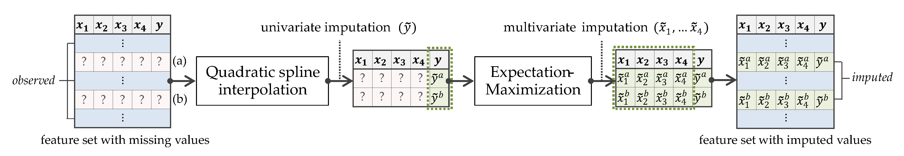
  • We devise a missing value imputation approach, which exploits both univariate and multivariate imputation techniques. Our approach first estimates the missing values of the target variable through the univariate imputation. Then, the rest of the missing values are replaced with plausible values by multivariate imputations.
  • To verify the forecasting model and proposed imputation approach, this paper includes an experiment for comparison with various imputation techniques.
The remainder of the paper is structured as follows: details on the EV charging dataset and its preprocessing are described in Section 2. Next, Section 3 defines the forecasting problem this paper addresses and explains the development of an LSTM-based forecasting model, which is a solution for that problem. Section 4 provides explanations of the existing data imputation techniques and our imputation approach. In Section 5, Experimental results about the data imputation and performance comparison with several imputation techniques are presented. Finally, Section 6 concludes this paper and explains the limitations of this study and future research directions.

2. EV Charging Data

The Korean Electric Power Corporation (KEPCO) has a great interest in the EV business, and currently operates a total of 2380 EV charging stations nationwide. As shown in Table 1, a dataset KEPCO provides for this study consists of a total of 13 data attributes, and a total of 445,704 data instances collected during the period from 1 January 2016 to 21 May 2018. To obtain refined data from the given dataset, we performed a number of corrections for invalid data (e.g., invalid value format and unexpected values). As a result, some data were excluded or replaced with corrected values.
Even with refined data that satisfies the validity, if there are a number of extreme outliers, it can distort the learning of the forecasting model and impair performance. Therefore, if the amount of charging is extremely small or large considering the charging time, it is treated as an outlier that should be removed from the dataset. As a metric for determining whether or not an outlier, the ratio of observation to a maximum amount of charging (OMC) is defined as follows:
O M C ( x ( i ) ) = x a m t ( i ) x m a x ( i ) × x c t ( i ) ,
where x ( i ) is the i-th data instance in the dataset, x a m t ( i ) is the amount of charging of x i , x m a x ( i ) is the maximum capacity of the charger corresponding to x ( i ) , and x c t ( i ) is the charging time of x ( i ) .
The denominator of OMC ( x m a x ( i ) × x c t ( i ) ) represents the maximum possible amount of charging within a give charging time. Therefore, for normal data, OMCs should be 1 or less. However, instead of removing all cases where OMC exceeded 1, we take into account minor measurement errors and apply outlier detection based on interquartile range (IQR), I Q R = Q 3 Q 1 , where Q 3 is the third quartile (75%) of the measured OMCs and Q 1 is the first quartile (25%). Based on IQR presented in Figure 2, outliers are defined as cases where OMC deviates from Q 1 or Q 3 by 1.5 · I Q R . Therefore, the upper bound ( f 3 ) and the lower bound ( f 1 ) for determining whether or not an outlier are defined as follows:
f 3 = Q 3 + 1.5 · I Q R
f 1 = Q 1 1.5 · I Q R
According to the equations above, if x o m c ( i ) f 3 , it is classified as a high outlier. In contrast, since an OMC cannot be negative, we do not apply f 1 and classify it as a low outlier when x o m c ( i ) 0 . As a result, we obtained a total of 399,390 data instances without outliers ( 89.6 % of the original dataset) as shown in Figure 3. A feature set, required to train the forecasting model is extracted from the resultant data.

3. EV Charging Station Load Forecasting

In this section, the EV load forecasting problem, which is mainly dealt with in this paper, is defined and the development procedure of an LSTM-based forecasting model to solve the problem is described.

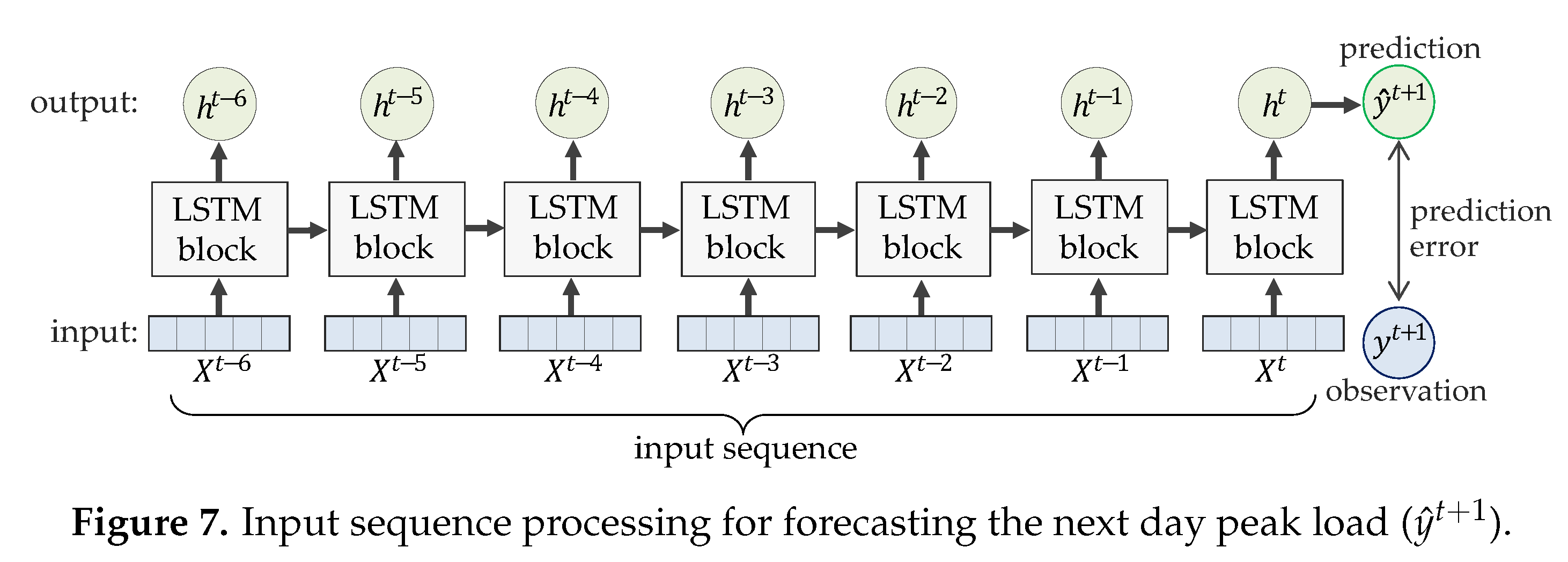
3.1. Forecasting Problem

Load forecasting is essential for electric power companies to make effective and timely decisions. Accurate long-term load forecasting is a great help in long-term power system operation and planning [11]. However, there is a limitation that acceptable forecasting results can be expected only when plentiful data accumulated over a long period of time is given. On the other hand, STLF (e.g., day-ahead load forecasting) not only reduces power generation costs but also plays an important role in operations to prevent undesirable incidents such as power blackouts.
In this paper, we address the daily peak load forecasting of EV charging stations, an instance of the STLF problem. Each EV charging station has a different charging pattern depending on the type of major users and spatial characteristics (e.g., vehicular flow). Each charging station’s forecasting allows us to understand the usage patterns of individual charging stations. Furthermore, by aggregating the forecasting results, electric power companies can effectively carry out the charging stations operation and charging facilities planning.
Before building a forecasting model, it is required to extract features that compose a training set from observations. Figure 4 shows the measurement of the daily peak load, which is the target variable of the forecasting model. Basically, a charging station operates multiple chargers, and the EV dataset consists of charging records collected from the individual chargers. Since the time intervals of these data recorded in an event-driven manner are not constant, it is mandatory to integrate the time series into a uniformed time granularity before constructing a forecasting model. In this regard, all load values are resampled into hourly loads and then an hourly charging station load is measured through the aggregation of hourly loads of chargers operated in a charging station. Consequently, the maximum of the measured hourly charging station loads is taken as the daily peak load of the charging station.

3.2. Development of the Forecasting Model

The concerns of this paper are two-fold. One is the development of a load forecasting model for EV charging stations using LSTM neural networks. The other one is the handling of missing values in the given dataset to let the forecasting model be more accurate. Regarding these concerns, the forecasting model is developed according to the procedure in Figure 5 and the following is a detailed description of each step.
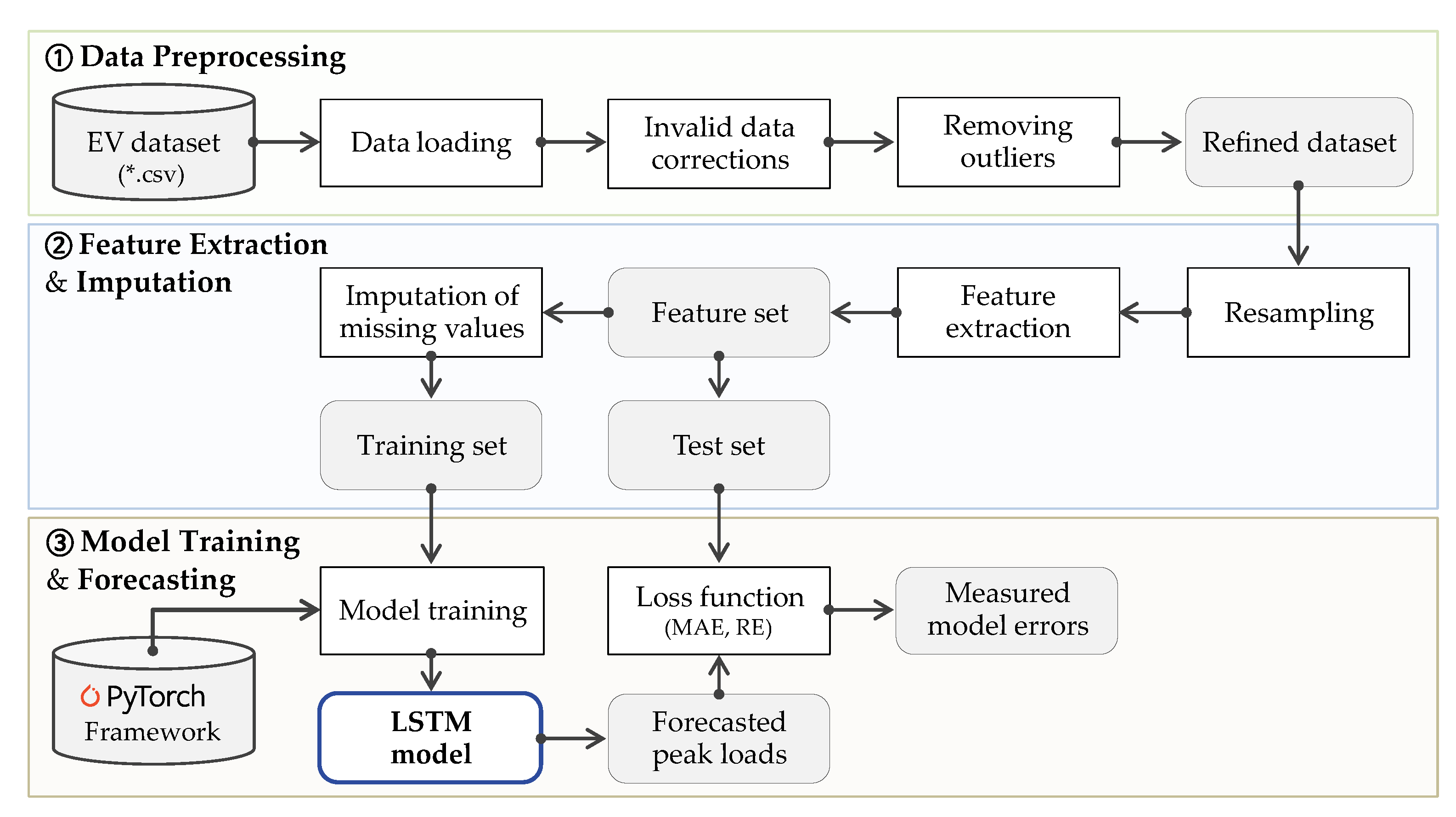
  • The given EV dataset is preprocessed (invalid data correction and outlier removal) to obtain a refined dataset. Details on the preprocessing are explained in Section 2 above.
  • A feature set is derived from the refined dataset through resampling and feature extraction. Including target values (i.e., daily peak loads), the whole features are extracted from the resampled hourly or daily data. This resampling results in missing values harmful for forecasting accuracy. To this end, several imputation techniques, including our approach are applied to generate new values of replacing the missing values. As a result, different training sets are generated depending on the imputation technique applied.
  • A number of LSTM-based forecasting models are built on each training set. Concretely, we exploit the libraries provided by PyTorch to train LSTM neural networks, which is a day-ahead forecast model for charging station peak loads. Finally, we verify the forecasting model and our imputation approach by comparing the forecasting results obtained from models of different imputation techniques.
Finally, we verify the prediction model and our imputation approach by comparing the prediction results obtained from models of different imputation techniques.
In order to make a training set from the dataset, we designed a feature set containing the following 7 features:
  • Charging station ID is a feature to learn charging patterns unique to individual charging stations. Through one-hot encoding, it is transformed into a binary vector of size N (the number of charging stations).
  • Day of the week is a feature for learning different charging patterns for each day of the week. It is also transformed into a binary vector of size 7 by one-hot encoding.
  • Numbers of normal/fast charges are the total numbers of charge of each type measured per day.
  • Amounts of normal/fast charges are the total energy amounts of charge of each type measured per day.
  • Daily peak load is the target variable, which the model aims to forecast.

3.3. Long Short-Term Memory

A vast amount of time series data strengthens the applicability of deep learning techniques to many types of time series forecasting problems. Recurrent Neural Network (RNN [12]) is one of the general deep learning models and is widely used for time series forecasting as well as natural language processing (NLP). However, since RNN has risks of vanishing/exploding gradients in the back-propagation process, it may not be the best option in modeling long-term dependencies of time series. As a variant of the RNN model, LSTM is composed of different gates that control deletion, addition, and output of information, and is known to have an advantage in long-term dependency modeling. Hence, the LSTM model has been successfully used in various domains, including not only the power system [13,14], but also the business process [15] and economy areas [16]. Therefore, in this paper, we develop a forecasting model of the EV charging station load based on the LSTM model.
As shown in Figure 6, an LSTM cell is a basic unit of LSTM networks and takes three elements as inputs. First, x t is a input vector at the time step t. Second, C t 1 is the internal state of the LSTM cell at the previous time step. As long-term stored information, it is continuously updated during the process of passing onto successive LSTM cells. Lastly, h t 1 is the hidden state at t 1 . As the output of the last cell, it is delivered to the next cell and the adjacent LSTM layer. Three gates in the LSTM cell process these inputs to obtain an updated cell state C t and new hidden state h t .
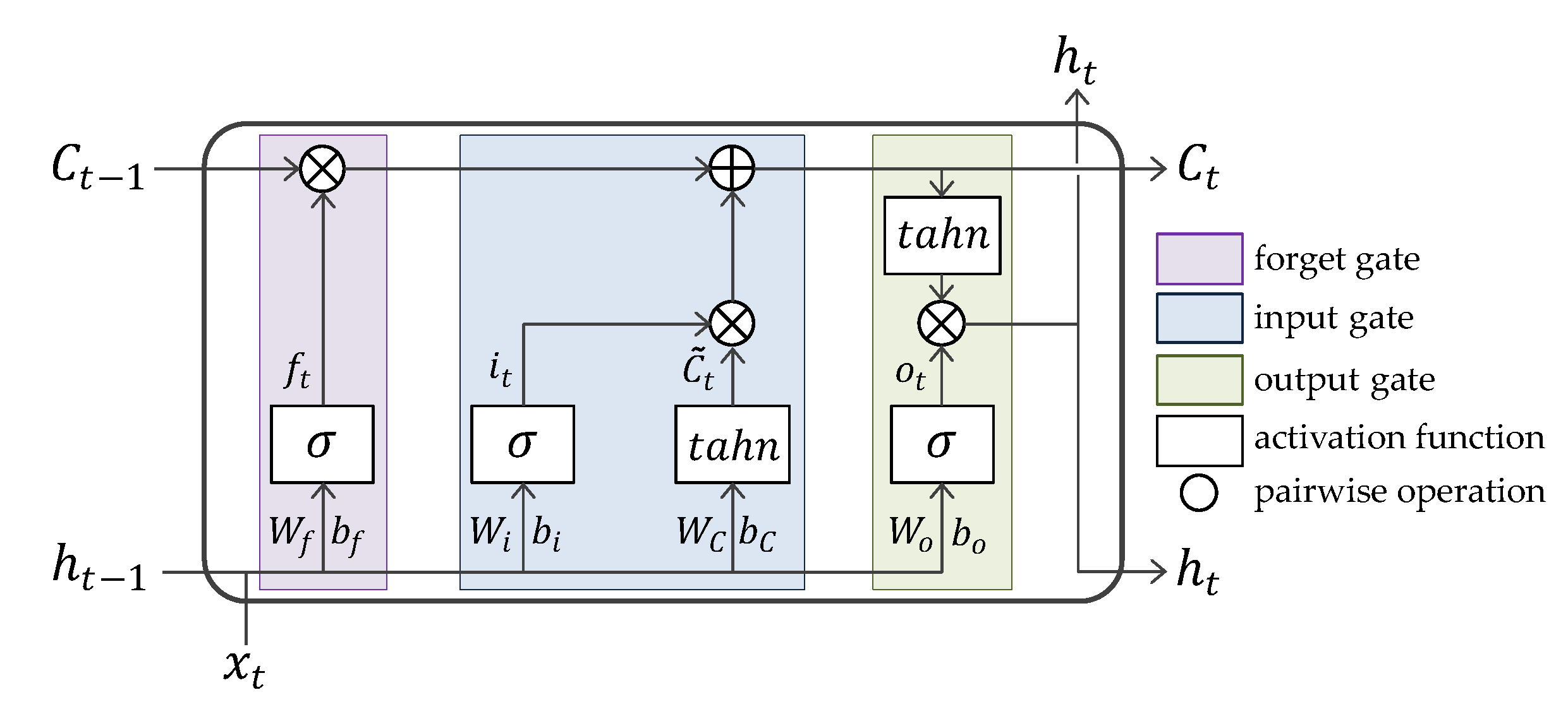
  • Forget gate decides what information should be removed from the cell state. Its gating function is implemented by a sigmoid neural net layer, σ with h t 1 and x t as inputs. σ outputs f t (between 0 and 1) that indicates a degree of how much this will discard the information. As an LSTM learns data, the weight values in this gate, W f and b f will be optimized.
    f t = σ ( W f · [ h t 1 , x t ] + b f ) .
  • Input gate decides what new information should be stored in the cell state. This includes two layers. First, a sigmoid layer outputs i t which means a weight of input information. Next, a hyperbolic tangent (called tahn) layer outputs a set of candidate values, C ˜ t , that could be added to the cell state. Then, the multiple of these two outputs i t · C ˜ t will be added to the cell state.
    i t = σ ( W i · [ h t 1 , x t ] + b i )
    C ˜ t = t a h n ( W C · [ h t 1 , x t ] + b C ) .
    The older cell state, C t 1 is replaced with the new cell state, C t through linear operations with the outputs of the two gates mentioned above.
    C t = C t 1 · f t + i t · C ˜ t .
  • Output gate is to decide a final output of an LSTM cell. First, a sigmoid layer calculates o t to scale the significance of output. Then, C t is put through tahn and multiply it by o t . This final result is a new hidden state h t and it is delivered to the next LSTM cell and neighboring hidden layer.
    o t = σ ( W o · [ h t 1 , x t ] + b o )
    h t = o t · t a n h ( C t ) .
Based on the LSTM model, we develop a daily peak load forecasting model which takes a sequence of features for 7 days as inputs ( X t 6 , . . . , X t ) and then predict the next day peak load ( y ^ t + 1 ) as shown in Figure 7. A prediction error is measured by differencing y ^ t + 1 with y t + 1 , an observed target value at time step t + 1 .

4. Data Imputation

Missing values found in the feature extraction may adversely affect the performance of the peak load forecasting model, so they should be corrected by an appropriate imputation process. This section introduces the existing techniques for the missing value imputation and describes our imputation approach which exploits both univariate and multivariate imputation techniques.

4.1. Existing Data Imputation Techniques

When we deal with real-world data, it is common to encounter missing values in the data. In many cases of this, missing values may become problematic as they distort the statistical properties of the data. Imputation is a way of replacing missing data with specific values. It can be an effective solution to build a robust predictive model from data containing missing values. This section introduces the two main classes of imputation methods (i.e., univariate and multivariate imputations) exploited in the performance evaluations of the paper.
In univariate imputation, the simplest technique is LOCF (stands for last observation carried forward), which carries forward the last observation before the missing data. Next observation carried backward (NOCB) is a similar approach to LOCF, which works by taking the first observation after the missing data and carrying it backward. These work well if there are strong correlations between data of consecutive time steps t i and t i 1 . Conversely, if there are huge differences between consecutive time steps, these are not appropriate to impute the missing values. Another imputation method is the interpolation of estimating intermediate values between two adjacent observed values by specific functions (e.g., linear, polynomial, and spline functions). Linear interpolation is a simple and lightweight method to connect two data points in a straight line, while it generally causes large errors. Polynomial and spline interpolations use high or low degree polynomials so that they produce smoother interpolants, replacing missing values with smaller errors than the linear interpolation.
Given data with massive columns, the multivariate imputation using the entire set of variables may be better than the univariate imputation. Since the multivariate imputation preserves the relationships with other variables, if the variables are highly correlated, it may produce more plausible values. The Expectation-Maximization (EM [17]) algorithm is one of the multivariate imputation methods to iteratively impute missing values based on the maximum likelihood estimation. EM imputations are prone to underestimate standard error. Therefore, this approach is only proper if the standard error of data is not vital. The k-Nearest Neighbors (k-NN) technique can also be applied to data imputation [18]. For each missing value, this technique finds the k closest neighbors to the observation with missing data and then imputing them with the mean value of the neighbors.

4.2. Proposed Imputation Approach

As described above, the training set consists of daily features resampled from the original EV dataset. In cases of charging stations with low data frequency, missing values are inevitably generated after the resampling process. In order to handle these missing values, we devise an imputation approach that combines the spline interpolation and EM algorithm; that is, the quadratic spline function first interpolates the missing values of the target variable (daily peak load). Next, the EM algorithm performs multivariate imputations on other features using the estimated target values as predictors. The reasons for devising the two-stage imputation approach are as follows. First, since missing values in the training set result from the resampling, on days when there is an absence of any charging events, all feature values except the charging station ID and day of the week are missing ( x 1 , . . . , x 4 and y in Figure 8). This means that the use of the multivariate imputation alone, which requires some of the observed values in a data instance, is not reasonable. Therefore, we use the spline interpolation method to construct target values of the missing part in a smooth shape instead of using EM or k-NN. Second, the other features (e.g., the amount of normal charging per day) have strong correlations with the target variable. Therefore, it is rational to perform multivariate imputation for the other features using the estimated target variable as a predictor ( y ˜ ). If the spline interpolation is used solely, the missing values of each feature are imputed regardless of the correlations. Thus, we use the EM algorithm as a multivariate imputation method in the second stage of imputation.

5. Experimental Results

The effect of imputing missing values is verified with two issues. One is about the issue of how similar values the imputation produces to the distribution of the original data. Another thing is how much the imputation process makes the forecasting model more accurate. In this regard, we first estimate the missing values in the EV dataset using several imputation techniques, including our imputation approach (QEM), which is the combination of the quadratic spline interpolation and the EM algorithm. Then, we conduct a performance comparison of forecasting models constructed from each imputed training set.
Data imputation and model training, are conducted with the experimental environment shown in Table 2. We built a peak load forecasting model based on the class of the LSTM model provided by the PyTorch Framework. In addition, we exploit the following Python packages for data imputation: Autoimpute (LOCF, NOCB and spline interpolation), Impyute (EM) and fancyimpute (k-NN).

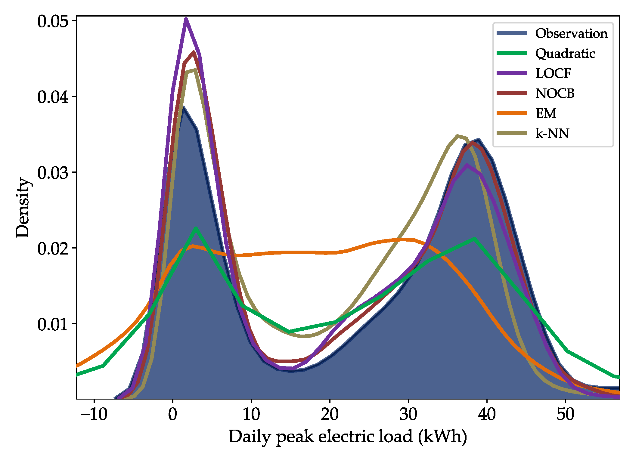
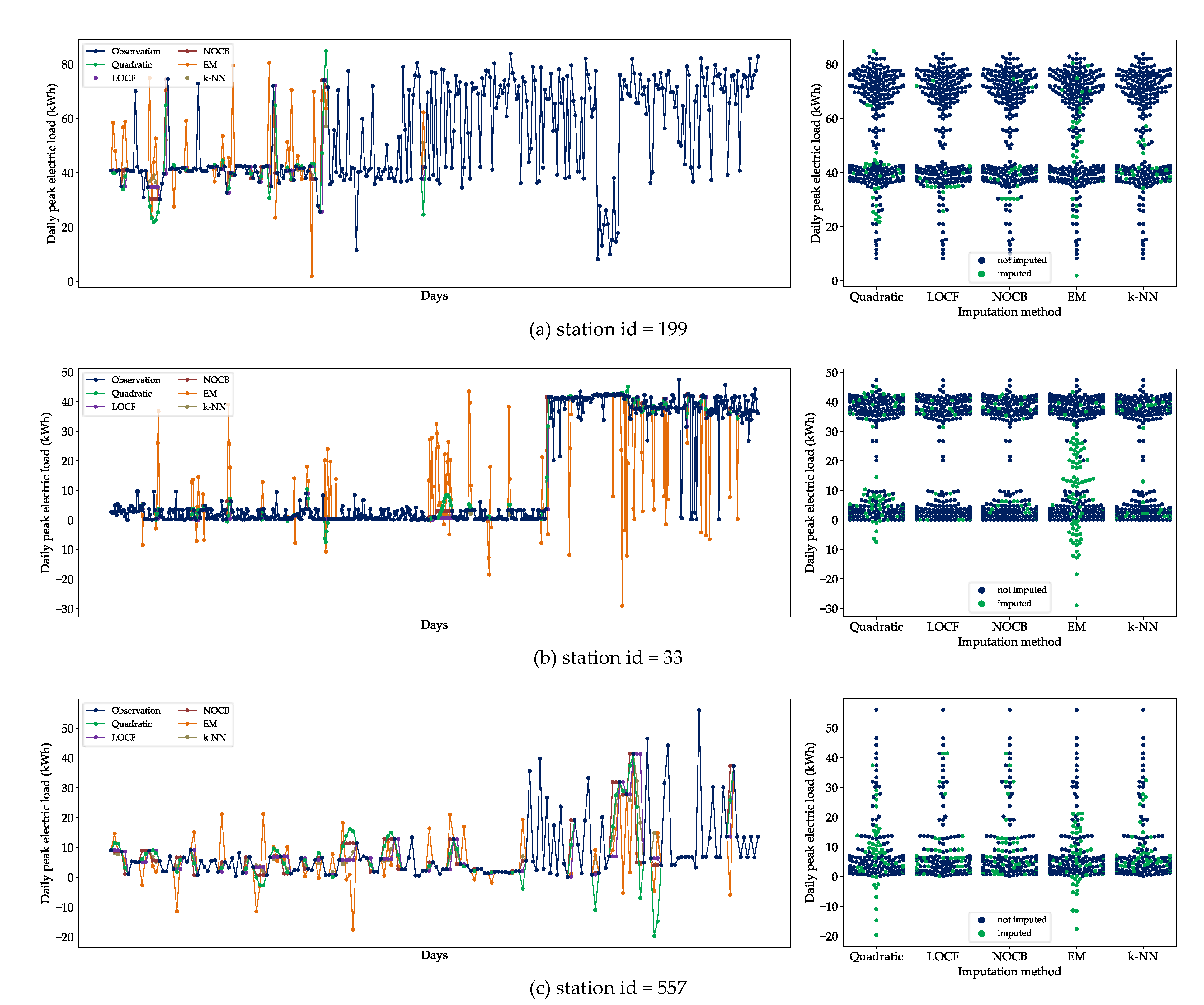
5.1. Missing Data Imputation

Table 3 represents a summary of the training set, including descriptive statistics of the measured daily peak loads ( μ , σ , 1Q, Med., and 3Q). In order to investigate the effect of the missing rate on imputation performance, we prepared a total of five training sets by the threshold of missing rate ( θ ). At θ = 0.1 , the training set contains only charging stations data with a missing rate under 10%. Therefore, this data is of high-quality that contains fewer missing values while the data size is smaller than other datasets, which might be insufficient for the model training. On the other hand, a training set with high θ is a larger data, including a lot of missing values.
In terms of the performance of imputation, it is significant how much the distribution of imputed values resembles with the population distribution. For datasets with few missing values, a distribution, highly similar to the population one might lead to a more accurate forecasting model. On the other hand, if a dataset contains a non-trivial amount of missing data, imputation values overfitting to the population have the potential of constructing a bad locally optimal model.
Figure 9 shows the distributions of target values obtained by performing imputation on the training set ( θ = 0.5 ). LOCF, NOCB, and k-NN generate substitute target variables that approximate the population distribution because they estimate based on adjacent observed values to the missing data. Our assumption derived from this result is that these overfitted results deteriorate a generalization of the model since the missing rate of the dataset is not trivial. On the contrary, EM produces imputation values that underfitting the population distribution, which may lead to a less accurate model. According to Figure 10, the imputed values by EM tend to be highly volatile and include many extreme negative values (especially Figure 10b). In addition, the swarm plots on the right of Figure 10 show a low correlation of the imputed values by EM with the population. The quadratic spline interpolation constructs target values in a balanced way across the population, and as a result, it outputs an imputation distribution with a moderate degree of similarity. Therefore, we use the quadratic method in the imputation for the target variable in order to follow the golden mean.

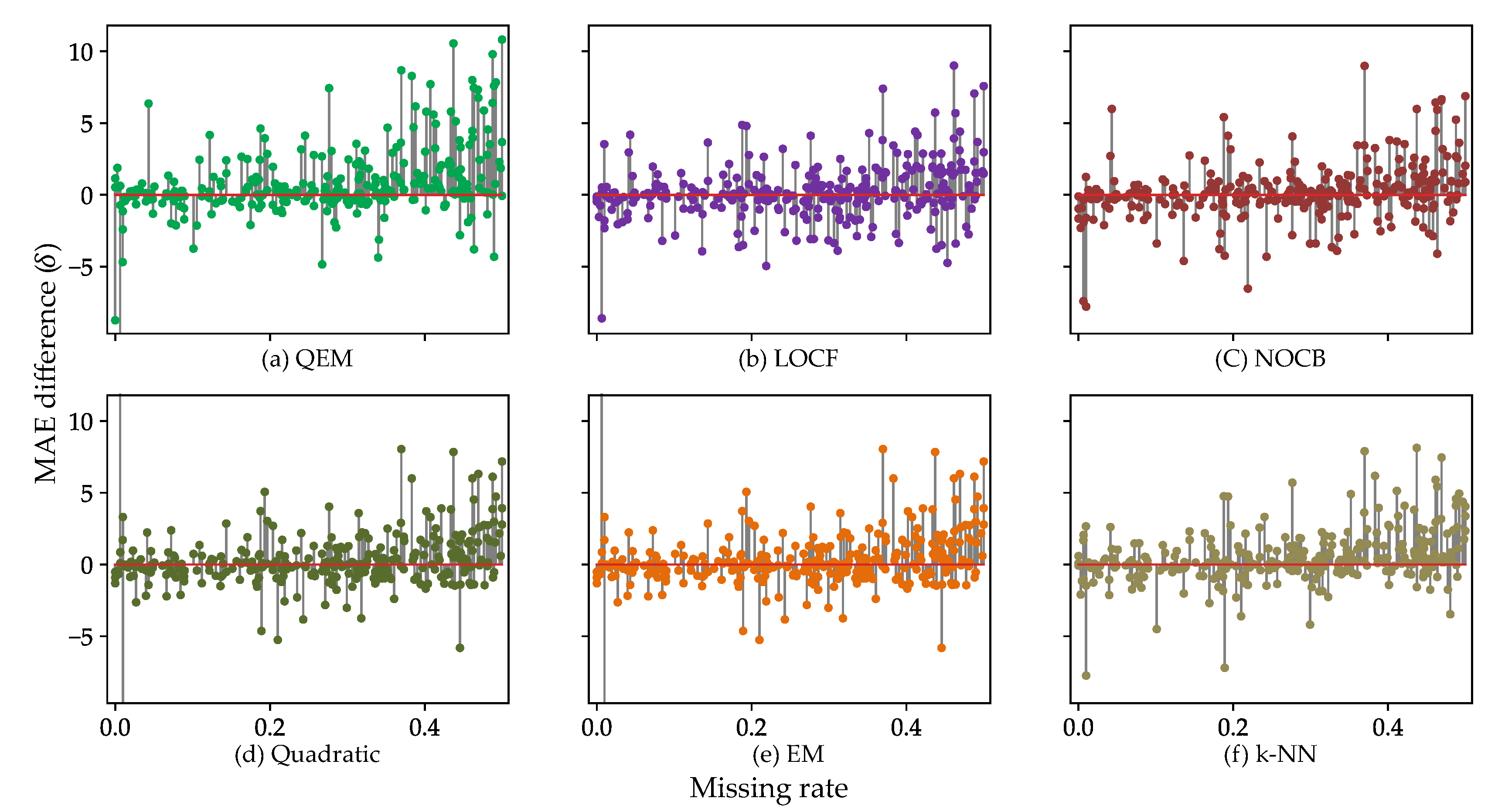
5.2. Performance Analysis

In order to evaluate the contribution of imputation to the model accuracy, an experiment for performance analysis is conducted according to the following: (1) a group of training sets is prepared by applying each imputation technique. (2) we obtain forecasting models derived from the training sets, each of which corresponds to each imputation technique. (3) we measure the prediction accuracy of the models and compare them to evaluate the effectiveness of the imputation techniques. All models based on LSTM are trained under the equivalent model hyperparameter setting as shown in Table 4. To model the weekly seasonality pattern, the sequence length required for each forecast is set to 7. In addition, we take the best accuracy observed for 300 epochs as a model accuracy.
The model accuracy is measured by the mean absolute error (MAE).
M A E = 1 n i = 1 n | y i y i ^ | ,
where n is number of sample data, y i is ith observation of daily peak load, and y ^ i is predicted value for y i . In addition, as a relative metric for performance comparison, we calculate the MAE difference ( δ ) between a forecasting model and the no-imputation model (NI).
δ = M A E ( N I ) M A E ( M ) ,
where M A E ( N I ) is the MAE of the NI model and M A E ( M ) is the MAE of a forecasting model with a particular imputation technique.
That is, a measured MAE difference determines whether the imputation technique improves (if δ > 0 ) or undermines (if δ < 0 ) the model performance compared with NI.
Figure 11 shows the comparison of δ of all charging stations using the training set with θ = 0.5 . Through the measured values of δ , it is verified that all the imputation techniques are superior to NI since they all resulted in more positive values of δ than negative ones. Overall, charging stations with low missing rates show that the effect of imputation is unclear, or even in some cases, the imputation results in worse performance. On the other hand, as the missing rate increases, the imputation models output a positive δ in many cases, and the magnitude of δ also surges. In particular, for charging stations with a high missing rate, QEM tends to achieve a greater performance improvement compared to the rest of the models including NI. This indicates that QEM is the most effective imputation method as the training set contains more missing values.
Table 5 summarizes the performance analysis results of the forecasting models, supported by imputation techniques for the training sets separately configured according to θ . In the case of QEM, our proposed imputation approach, it achieved the finest results in terms of forecast accuracy in three cases ( θ = 0.2 , 0.4 , and 0.5 ). In particular, on the cases of high missing rates ( θ = 0.4 and 0.5 ), it was confirmed that the numerous missing values widen the performance gap between QEM and other models ( δ = 0.347 and 0.933 respectively). Compared to NI, QEM reduced MAE by up to 9.8% at θ = 0.1 (NI: 9.47 ± 0.057 and QEM: 8.537 ± 0.076 ). In contrast, for the training set of θ = 0.1 , QEM outputs a negative MAE difference ( δ = 0.077 ), indicating that the imputation process of QEM adversely affected the model performance compared to NI not supported by imputation. Compared to the quadratic spline interpolation, since the results of QEM are superior in all cases except for the case of θ = 0.1 , we verified that our approach of performing multivariate imputation after univariate imputation was appropriate for the missing values in the EV dataset.
In the results of EM and k-NN as multivariate imputation models, each of them showed the best performance in one case (EM for θ = 0.3 and k-NN for θ = 0.1 ). If there are variables within the dataset that can be used as predictors for the imputation of other variables, the forecasting model may benefit from multivariate imputation. In the given dataset, however, there are no predictors available for the data instances where the missing occurred, and therefore EM and k-NN were not better than QEM combining with univariate imputation.
In the cases of LOCF and NOCB, which are the simplest imputation techniques, NOCB yielded better results than LOCF for low missing rates ( θ = 0.1 and 0.2 ), and LOCF got the better of NOCB at high missing rates ( θ = 0.3 , 0.4 and 0.5 ). Since they impute substitute values by linearly connecting the data points just before or after the missing part, they are not suitable for long-interval consecutive missing values. Overall, both techniques underperformed compared with QEM, EM, and k-NN.
Putting the results of all the cases together, we verified that QEM is a proper method to elicit the performance improvement of the forecasting model from EV charging data with a lot of missing values. However, the results showed that QEM is not attractive for stable data with few missing values, so there is a limitation that the model performance is dependent on the missing rate. On the one hand, despite the application of the imputation techniques for missing values, the forecasting accuracy is still a challenge. In order to obtain a model with an acceptable level of accuracy, it is necessary to improve the quality of the EV charging data and to devise a sophisticated imputation method that performs well regardless of the missing rate.

6. Conclusions

In this paper, we proposed an LSTM-based prediction model for daily peak load forecasting of EV charging stations. In addition, in order to mitigate the degradation of forecast accuracy due to missing values, we devised an imputation method appropriate for the EV charging dataset. Similar to the previous study [9], the EV dataset has the dominant type of missingness, indicating that, for instances in which the missing occurs, the values of all variables that could be predictors for other variables are missing. For this, our imputation approach, QEM was designed to first construct the values of the target variable though the quadratic spline interpolation, and then perform multivariate imputation by EM using the estimated target values as predictors to fill the remaining variables.
The experimental results obtained through the performance comparison including several imputation techniques showed that QEM has the best improvements in forecasting accuracy for the majority of training sets. In addition, compared to the strategy without applying imputation (NI), QEM resulted in reduced forecasting errors of up to 9.8%. However, for data with few missing values, QEM did not show a clear advantage over other imputation techniques, even for the dataset with θ = 0.1 , it underperformed NI. To overcome this shortcoming, we are planning to improve the imputation method to obtain a reliable forecasting model that works well regardless of missing rates.

Author Contributions

Conceptualization, B.L., H.L. and H.A.; Data curation, B.L. and H.L.; Investigation, H.A.; Methodology, B.L. and H.A.; Software, H.L. and H.A.; Supervision, B.L. and H.L.; Writing—original draft, B.L. and H.A.; Writing—review & editing, H.L. All authors have read and agreed to the published version of the manuscript.

Funding

This work was supported by the National Research Foundation of Korea (NRF) grant funded by the Korea government (Ministry of Science and ICT, Grant No. NRF-2018R1C1B5086414).

Conflicts of Interest

The authors declare no conflict of interest.

Abbreviations

The following abbreviations are used in this manuscript:
CNNConvolutional Neural Network
EMExpectation-Maximization
EVElectric Vehicle
k-NNk-Nearest Neighbors
KEPCOKorean Electric Power Corporation
LOCFLast Observation Carried Forward
LSTMLong Short-Term Memory
MAEMean Absolute Error
NINo Imputation
NLPNatural Language Processing
NOCBNext Observation Carried Backward
RFRandom Forest
RNNRecurrent Neural Network
STLFShort-Term Load Forecasting
SVRSupport Vector Regression

References

  1. Clairand, J.-M.; Álvarez-Bel, C.; Rodríguez-García, J.; Escrivá-Escrivá, G. Impact of electric vehicle charging strategy on the long-term planning of an isolated microgrid. Energies 2020, 13, 3455. [Google Scholar] [CrossRef]
  2. Lee, J.; Lee, E.; Kim, J. Electric vehicle charging and discharging algorithm based on reinforcement learning with data-driven approach in dynamic pricing scheme. Energies 2020, 13, 1950. [Google Scholar] [CrossRef] [Green Version]
  3. Jain, A.; Satish, B. Short term load forecasting by clustering technique based on daily average and peak loads. In Proceedings of the 2009 IEEE Power Energy Society General Meeting, Calgary, AB, Canada, 26–30 July 2009; pp. 1–7. [Google Scholar]
  4. Dong, X.; Qian, L.; Huang, L. Short-term load forecasting in smart grid: A combined CNN and K-means clustering approach. In Proceedings of the 2017 IEEE International Conference on Big Data and Smart Computing, Jeju, Korea, 13–16 February 2017; pp. 119–125. [Google Scholar]
  5. Arias, M.B.; Kim, M.; Bae, S. Prediction of electric vehicle charging-power demand in realistic urban traffic networks. Appl. Energy 2017, 195, 738–753. [Google Scholar] [CrossRef]
  6. Majidpour, M.; Qui, C.; Chu, P.; Pota, H.R.; Gadh, R. Forecasting the EV charging load based on customer profile or station measurement? Appl. Energy 2016, 163, 134–141. [Google Scholar] [CrossRef] [Green Version]
  7. Savari, G.F.; Krishnasamy, V.; Sathik, J.; Ali, Z.M.; Aleem, S.H.E.A. Internet of Things based real-time electric vehicle load forecasting and charging station recommendation. ISA Trans. 2020, 97, 431–447. [Google Scholar] [CrossRef] [PubMed]
  8. Ryu, S.; Noh, J.; Kim, H. Deep neural network based demand side short term load forecasting. Energies 2017, 10, 3. [Google Scholar] [CrossRef]
  9. Majidpour, M.; Chu, P.; Gadh, R.; Pota, H.R. Incomplete data in smart grid: Treatment of missing values in electric vehicle charging data. In Proceedings of the 2014 International Conference on Connected Vehicles and Expo, Vienna, Austria, 3–7 November 2014; pp. 1041–1042. [Google Scholar]
  10. Hochreiter, S.; Schmidhuber, J. Long short-term memory. Neural Comput. 1997, 9, 1735–1780. [Google Scholar] [CrossRef] [PubMed]
  11. AlRashidi, M.R.; EL-Naggar, K.M. Long term electric load forecasting based on particle swarm optimization. Appl. Energy 2010, 87, 320–326. [Google Scholar] [CrossRef]
  12. Rumelhart, D.E.; Hinton, G.E.; Williams, R.J. Learning representations by back-propagating errors. Nature 1986, 323, 533–536. [Google Scholar] [CrossRef]
  13. Kong, W.; Dong, Z.Y.; Jia, Y.; Hill, D.J.; Xu, Y.; Zhang, Y. Short-term residential load forecasting based on LSTM recurrent neural network. IEEE Trans. Smart Grid 2017, 10, 841–851. [Google Scholar] [CrossRef]
  14. Choi, H.; Ryu, S.; Kim, H. Short-term load forecasting based on ResNet and LSTM. In Proceedings of the 2018 IEEE International Conference on Communications, Control, and Computing Technologies for Smart Grids, Aalborg, Denmark, 29–31 October 2018; pp. 1–6. [Google Scholar]
  15. Ham, S.H.; Ahn, H.; Kim, K.P. LSTM-based business process remaining time prediction model featured in activity-centric normalization techniques. J. Internet Comput. Serv. 2020, 21, 83–92. [Google Scholar]
  16. Kim, H.Y.; Won, C.H. Forecasting the volatility of stock price index: A hybrid model integrating LSTM with multiple GARCH-type models. Expert Syst. Appl. 2018, 103, 25–37. [Google Scholar] [CrossRef]
  17. Moon, T.K. The expectation-maximization algorithm. IEEE Signal Proc. Mag. 1996, 13, 47–60. [Google Scholar] [CrossRef]
  18. Malarvizhi, M.R.; Thanamani, A.S. K-nearest neighbor in missing data imputation. Int. J. Engineer. Res. Dev. 2012, 5, 5–7. [Google Scholar]
  19. Pandas. Available online: https://pandas.pydata.org (accessed on 15 August 2020).
  20. Numpy. Available online: https://numpy.org (accessed on 15 August 2020).
  21. Autoimpute. Available online: https://kearnz.github.io/autoimpute-tutorials (accessed on 15 August 2020).
  22. Fancyimpute. Available online: https://github.com/iskandr/fancyimpute (accessed on 15 August 2020).
  23. Impyute. Available online: https://impyute.readthedocs.io/en/latest (accessed on 15 August 2020).
  24. Scikit-Learn: Machine Learning in Python. Available online: https://scikit-learn.org/stable (accessed on 15 August 2020).
  25. Matplotlib: Python Plotting. Available online: https://matplotlib.org (accessed on 15 August 2020).
  26. Seaborn: Statistical Data Visualization. Available online: https://seaborn.pydata.org (accessed on 15 August 2020).
Figure 1. Growth of the electric vehicle (EV) market in Korea.
Energies 13 04893 g001
Figure 2. Interquartile range (IQR)-based outlier detection.
Energies 13 04893 g002
Figure 3. Refined data after removing the outliers.
Energies 13 04893 g003
Figure 4. Measurement of the daily peak load at a charging station.
Energies 13 04893 g004
Figure 5. The overall procedure for developing the forecasting model.
Energies 13 04893 g005
Figure 6. The structure of an long short-term memory (LSTM) cell.
Energies 13 04893 g006
Figure 7. Input sequence processing for forecasting the next day peak load ( y ^ t + 1 ).
Energies 13 04893 g007
Figure 8. Imputation approach.
Energies 13 04893 g008
Figure 9. Density estimation of the observations and imputed values.
Energies 13 04893 g009
Figure 10. Imputation results in the sample station data.
Energies 13 04893 g010
Figure 11. MAE differences between each model and NI.
Energies 13 04893 g011
Table 1. Descriptions of the EV dataset.
AttributeData TypeDescription
headquaterstringa total of 17 headquaters (e.g., Seoul HQ)
divisionstringa total of 193 divisions (e.g., Div. of Mapo-Yongsan)
charging station IDstringa total of 2380 stations
address of charging stationstring
charger IDinta total of 6010 chargers
charger typestringnormal or fast
maximum capacity of chargerfloatunit: kilowatt (kW)
amount of chargingfloatunit: kilowatt hour (kWh)
start time of chargingdatetime
end time of chargingdatetime
charging timedatetimeformat: hh:mm:ss
Table 2. Experimental setup.
AttributeDescription
GPUNVIDIA GeForce 2080 RTX Super (8GB)
CPUIntel Core i9-9900
RAM32GB
OSWindows 10 Pro 64bit
Deep learning frameworkPyTorch (1.1.0), Cuda (v10.2)
Python librariespandas [19] (data I/O and manipulation)
NumPy [20] (numerical operations)
Autoimpute [21], fancyimpute [22], Impyute [23] (data imputation)
scikit-learn [24] (feature normalization)
Matplotlib [25], seaborn [26] (visualization)
Table 3. Summary of the training set.
θ Num. of StationsData SizeNum. of Missing ValuesMissing Rate μ σ 1QMed.3Q
0.15219,6608534.34%41.22126.16030.21939.81551.302
0.29637,82037059.80%35.66024.14422.34337.31043.924
0.315565,59110,68416.29%31.08223.1796.75535.01741.852
0.422396,20421,21822.06%29.54821.9736.46734.02241.000
0.5303135,20738,79928.70%28.38621.2126.21033.23140.480
θ : threshold of missing rate, μ : mean, σ : standard deviation, 1Q, 3Q: 1st/3rd quartiles, Med.: median.
Table 4. Hyperparameters for the model training.
Hidden LayersHidden NodesSequence LengthOptimizerLearning RateDrop RateEpochs
31507Adam0.0010.5300
Table 5. Summary of the performance analysis.
θ NIQEMLOCFNOCBQuadraticEMk-NN
0.1MAE 11.371 ± 0.191 11.448 ± 0.012 11.936 ± 0.003 11.522 ± 0.187 11.336 ± 0.159 11.306 ± 0.046 11 . 268 ± 0 . 001
δ 0.077 0.565 0.151 0.035 0.065 0 . 103
0.2MAE 10.227 ± 0.03 10 . 076 ± 0 . 036 10.228 ± 0.044 10.174 ± 0.056 10.284 ± 0.029 10.213 ± 0.099 10.509 ± 0.026
δ 0 . 151 0.001 0.053 0.057 0.014 0.282
0.3MAE 9.798 ± 0.007 9.681 ± 0.008 9.701 ± 0.022 9.726 ± 0.046 9.802 ± 0.047 9 . 587 ± 0 . 057 9.63 ± 0.004
δ 0.117 0.097 0.072 0.004 0 . 211 0.168
0.4MAE 9.576 ± 0.031 9 . 229 ± 0 . 05 9.363 ± 0.085 9.515 ± 0.106 9.487 ± 0.088 9.278 ± 0.039 9.281 ± 0.067
δ 0 . 347 0.213 0.061 0.089 0.298 0.295
0.5MAE 9.47 ± 0.057 8 . 537 ± 0 . 076 9.192 ± 0.04 9.277 ± 0.038 9.122 ± 0.027 8.944 ± 0.135 8.982 ± 0.005
δ 0 . 933 0.278 0.193 0.348 0.526 0.488

