Compressed Machine Learning Models for the Uncertainty Quantification of Power Distribution Networks

Abstract

Today’s spread of power distribution networks, with the installation of a significant number of renewable generators that depend on environmental conditions and on users’ consumption profiles, requires sophisticated models for monitoring the power flow, regulating the electricity market, and assessing the reliability of power grids. Such models cannot avoid taking into account the variability that is inherent to the electrical system and users’ behavior. In this paper, we present a solution for the generation of a compressed surrogate model of the electrical state of a realistic power network that is subject to a large number (on the order of a few hundreds) of uncertain parameters representing the power injected by distributed renewable sources or absorbed by users with different consumption profiles. Specifically, principal component analysis is combined with two state-of-the-art surrogate modeling strategies for uncertainty quantification, namely, the least-squares support vector machine, which is a nonparametric regression belonging to the class of machine learning methods, and the widely adopted polynomial chaos expansion. Such methods allow providing compact and efficient surrogate models capable of predicting the statistical behavior of all nodal voltages within the network as functions of its stochastic parameters. The IEEE 8500-node test feeder benchmark with 450 and 900 uncertain parameters is considered as a validation example in this study. The feasibility and strength of the proposed method are verified through a systematic assessment of its performance in terms of accuracy, efficiency, and convergence, based on reference simulations obtained via classical Monte Carlo analysis.

1. Introduction

Nowadays, the reliability assessment of a power distribution network (PDN) must incorporate the effects of the unavoidable fluctuation of load consumption on the node voltages. Typical examples are represented by the pervasive spread of distributed generators (DGs), for which the injected power depends on (1) weather conditions; (2) the impact of hubs for charging electrical vehicles, located in different points of the network; and (3) the unpredictable user behavior, in a scenario in which both users and buildings play an active role in the continuous monitoring of the fluid electricity fees, and modify their power consumption accordingly [1,2,3,4]. Therefore, the inherent statistical nature of the problem makes a deterministic interpretation unsuitable, and demands for stochastic methodologies for the uncertainty quantification (UQ) [5,6,7].

Monte Carlo (MC) simulation represents the most straightforward way of performing a statistical load flow analysis of a power grid with uncertain loads [8,9,10,11,12,13,14]. The underlying idea is to run a large set of deterministic simulations in which the power level of each uncertain node is drawn according to its probability density function (PDF). Despite its simplicity and accuracy, a naive MC simulation turns out to be extremely expensive in terms of simulation time because of its slow convergence rate. Indeed, it requires a huge number (typically, on the order of thousands) of samples, which makes its direct application to a full-computational model unfeasible for realistic scenarios.

This reason motivated the growing interest, expressed by the electrical and electronic engineering community during the last fifteen years, in the development of enhanced and efficient alternatives to MC simulation for both the worst-case and the statistical assessment of the stochastic responses of complex systems [15,16,17]. Among the state-of-the-art approaches, polynomial chaos expansion (PCE) can be considered as the reference technique for UQ [18,19]. The underlying idea is to represent the relationship between the uncertain variables and the outputs of interest in terms of an expansion of suitable orthogonal polynomial basis functions [20]. The expansion coefficients can be computed by means of least-square regression, starting from a limited set of random “training samples” obtained from the full-computational model. The resulting surrogate model allows an expedite statistical assessment of the original system. However, similar to most parametric regression methods, in which the number of unknowns depends on the number of input parameters, the application of classical PCE becomes impractical for systems with a large number of uncertain parameters, as the number of basis functions, and thus of regression coefficients, grows exponentially. For example, a second-order PCE for 500 uncertain variables requires the estimation of ~250k coefficients: this is the so-called “curse of dimensionality”. Fortunately, owing to the sparsity-of-effects principle, most of the model coefficients are in practice negligible. This led to the development of sparse algorithms [21,22,23,24], which reduce the number of unknowns and allow dealing with hundreds of uncertain variables (see, e.g., in [25]).

Recently, advanced machine learning (ML) methods [26,27] have been also employed for the UQ of several realistic problems in electrical engineering [28,29]. Specifically, flexible and powerful ML regressions, such as support vector machine (SVM) [30,31], least-square support vector machine (LS-SVM) [32], and Gaussian processes [33], were effectively applied to build accurate surrogate models starting from a limited set of training samples [34,35,36,37]. The resulting surrogate model is able to predict both the deterministic and the stochastic behavior of the system output for any configuration of the uncertain input parameters. As opposed to PCE-based methods, the above ML techniques allow constructing nonparametric surrogates in which the number of regression unknowns is independent from the dimensionality of the input space (i.e., the number of uncertain parameters) [32,33]. Therefore, ML methods appear to be an attractive solution to mitigate the curse of dimensionality and provide a powerful alternative for tackling UQ problems with a huge number (e.g., thousands) of variables.

Based on the above discussion, the load flow analysis of a power distribution network represents a perfect example for which sparse PCE methods and ML techniques can be applied. Indeed, the network typically involves thousands of nodes and a very large number of possible uncertain variables. This is an extreme situation for which MC simulation is definitely inefficient, and yet traditional surrogate modeling techniques like standard PCE fail to deal with more than a few tens of uncertain parameters (see, e.g., in [38]). On the other hand, the direct application of the aforementioned advanced modeling methods is limited in this case by the huge number of output variables of interest. As the model parameters have to be optimized separately for each output variable, the computational complexity is proportional to the number of variables of interest which, for a power distribution network, usually amount to thousands of steady-state voltages at the network nodes. To overcome this detrimental limitation, principal component analysis (PCA) is used to compress the number of output variables that need to be effectively modeled [39], thus reducing the model building cost typically by some order of magnitude.

In particular, a large benchmark network based on the Institute of Electrical and Electronics Engineers (IEEE) 8500-node test feeder [40] is considered in this paper. Sparse PCE and LS-SVM regression are employed in conjunction with PCA compression to build a surrogate model of the nodal voltages of the power distribution network with a large number of uncertain parameters consisting of power loads and renewable sources. The performance of the proposed modeling scheme in terms of efficiency, accuracy, and convergence, is thoroughly investigated by means of two scenarios with 450 and 900 uncertain parameters.

The remainder of this paper is organized as follows. Section 2 outlines the goal of this work. Section 3 presents the simulation scheme that is used to carry out the power-flow analysis. In Section 4.1, the mathematical background of LS-SVM regression and sparse PCE, as well as the PCA compression, are briefly introduced. The performance of the proposed methodology is investigated in Section 5 by considering the UQ of a complex benchmark network with an increasing number of training samples and of uncertain parameters. Finally, Section 6 concludes the paper.

2. Goal Statement

Without loss of generality, we consider the IEEE-8500 distribution feeder benchmark network [40], depicted in Figure 1, as test case for the proposed analysis. It is a three-phase radial distribution network consisting of medium and low voltage levels, with unbalanced loads, transformers, capacitors, and regulators. The network is modified by the addition of 200/400 photovoltaic (PV) distributed generators randomly connected at the load nodes. The uncertain variables are the values of real power for a set of $N_{load}$ network loads and $N_{pv}$ PV generators, thus leading to a problem with $d=(N_{load}+N_{pv})$ uncertain parameters, which we denote with vector $\mathbf{x}={[x_1,\dots ,x_d]}^{\mathsf{T}}\in {\mathbb{R}}^d$.

The goal of our analysis is to quantify the impact of the uncertain parameters on the magnitude of the network nodal voltages, hereafter referred to as the output vector $\mathbf{y}={[y_1,\dots ,y_M]}^{\mathsf{T}}\in {\mathbb{R}}^M$. The output vector is an implicit function of $\mathbf{x}$, which we denote as

$$\mathbf{y}=\mathcal{M}\left(\mathbf{x}\right),$$

(1)

where $\mathcal{M}:{\mathbb{R}}^d\to {\mathbb{R}}^M$ generically indicates the full-computational model that is used to calculate $\mathbf{y}$ for a given configuration of $\mathbf{x}$. It is important to point out that we are targeting applications with $d\sim {10}^2,{10}^3$ and $M\sim {10}^3,{10}^4$, for which both standard and advanced surrogate modeling techniques usually fail.

3. Power-Flow Analysis

This section describes the simulation technique that is used in the context of this paper as the full-computational model (1) for the power flow analysis of a power distribution network. The approach is illustrated in Figure 2. It relies on a nonlinear circuital interpretation of the distribution network in the phasor domain, see, for example, Figure 3a, in which the loads are replaced by nonlinear blocks characterized by their real and reactive power [41]. The circuit in Figure 3a can be interpreted as the interconnection of a linear and a nonlinear part, as shown in Figure 3b. The linear part is composed by the two-terminal elements $Y_n$, which represent the lumped (e.g., $RL$) equivalents of the transmission lines, and by the ideal feeding voltage source. The loads are considered as nonlinear elements in which the I-V characteristics are defined according to their complex absorbed power. As an examples, the I-V characteristic for the n-th load reads

$${\widehat{I}}_n=f({\widehat{V}}_n;P_n,Q_n,\omega )={\left(\frac{P_n+j{Q}_n}{{\widehat{V}}_n}\right)}^{*},$$

(2)

where ${\widehat{I}}_n$ and ${\widehat{V}}_n$ are the phasors of the node voltage and current, respectively, while $P_n$ and $Q_n$ represent the real and reactive power absorbed by the node, respectively. The resulting nonlinear circuital equivalent can be also reinterpreted as shown in Figure 3c, where the linear and nonlinear blocks have been decoupled by means of controlled sources. This schematic is readily described in matrix form by means of the modified nodal analysis (MNA) formulation [42].

Unfortunately, a closed-form solution of the resulting nonlinear equation is not available, and a numerical solution must be considered. To this aim, the problem is solved by means of the waveform relaxation technique [43], leading to the simplified circuital interpretation shown in Figure 3d. The above circuital interpretation turns out to be equivalent to a fixed-point iteration scheme:

$$\begin{array}{c}\hfill \left\{\begin{array}{c}\widehat{\mathbf{M}}{\widehat{\mathbf{W}}}^{\left(i\right)}={\widehat{\mathbf{A}}}_0+{\widehat{\mathbf{A}}}^{\left(i\right)}\hfill \\ {\widehat{\mathbf{A}}}^{(i+1)}=\widehat{\mathbf{A}}({\widehat{\mathbf{W}}}^{\left(i\right)}),\hfill \end{array}\right.\end{array}$$

(3)

where, with reference to Figure 3d,

• $\widehat{\mathbf{M}}$ is the MNA matrix, which is constructed by circuit inspection and incorporates the characteristics of the circuit elements;
• $\widehat{\mathbf{W}}$ is a complex vector collecting the nodal voltages ${\widehat{V}}_n^{\left(i\right)}$;
• ${\widehat{\mathbf{A}}}^{\left(i\right)}$ is a vector collecting the amplitude ${\widehat{I}}_n^{\left(i\right)}$ of the independent current sources; and
• ${\widehat{\mathbf{A}}}^{(i+1)}$ is a vector collecting the phasors of the currents that flow through the controlled voltage sources.

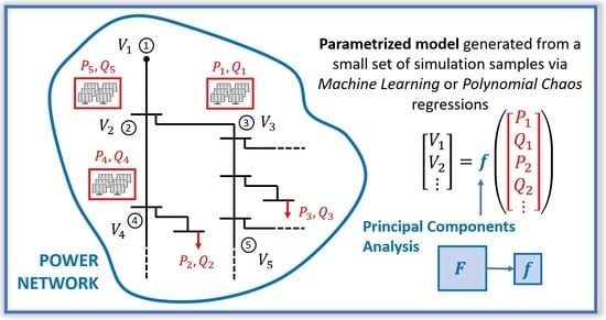
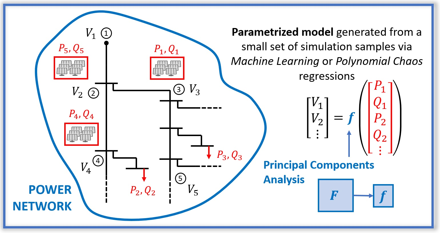
Iterating (3) over index i leads to the following update rule.

$$\begin{array}{c}\hfill {\widehat{\mathbf{W}}}^{(i+1)}={\widehat{\mathbf{M}}}^{-1}({\widehat{\mathbf{A}}}_0+\widehat{\mathbf{A}}({\widehat{\mathbf{W}}}^{\left(i\right)})).\end{array}$$

(4)

The iterations are terminated when a given error threshold $\epsilon$ is reached, such that

$$\parallel {\widehat{\mathbf{W}}}^{(i+1)}-{\widehat{\mathbf{W}}}^{\left(i\right)}{\parallel }_{\infty }\le \epsilon .$$

(5)

As discussed in [41], the linear portion of the system needs to be solved only once at the beginning of the iteration (i.e., the inverse matrix ${\widehat{\mathbf{M}}}^{-1}$ must be computed once), and the computation of the Jacobian matrix of the system is not required, thus simplifying the implementation. The circuital interpretation of Figure 3d is readily implemented in any SPICE-type solver to obtain the AC solution at a single frequency point.

The outlined simulation framework is implemented in MATLAB (R2019b, Mathworks, USA). It has been thoroughly validated and proven to be a viable solution for large networks [41]. At this point, it should be noted that any deterministic tool for load-flow analysis could be alternatively adopted as full-computational model.

4. Surrogate Models

We introduce here the surrogate models that will be used in conjunction with the power-flow analysis method of Section 3 for the UQ of the distribution network introduced in Section 2. For the sake of simplicity, we base the discussion on a system (1) with a scalar output (i.e., $M=1$), and we assume that a set of L training pairs ${\left\{({\mathbf{x}}_i,y_i)\right\}}_{i=1}^L$ is available, where $y_i=\mathcal{M}\left({\mathbf{x}}_i\right)\in \mathbb{R}$, $\forall i=1,\dots ,L$. At this stage, it is understood that for a multi-output system ($M>1$), the procedure is repeated for each output component. A compression strategy is introduced later, in Section 4.3, to handle multi-output systems more effectively.

4.1. LS-SVM Regression

This section introduces the underlying idea and the essential mathematical background of the LS-SVM regression in its primal and dual space formulations [32], along with its application to the construction of a surrogate model for UQ. It is worth mentioning that the code for the construction of LS-SVM surrogate models is available within the MATLAB toolbox LS-SVMLab, (version 1.8) [44].

4.1.1. Primal Space Formulation

The primal space formulation of the LS-SVM suggests approximating the actual responses of (1) with the surrogate model

$$\begin{array}{c}\hfill y\approx {\mathcal{M}}_{LS-SVM}\left(\mathbf{x}\right)=\sum _{n=1}^N{w}_n{\varphi }_n\left(\mathbf{x}\right)=\langle \mathbf{w},\mathit{\varphi }\left(\mathbf{x}\right)\rangle +b,\end{array}$$

(6)

where $\mathit{\varphi }\left(\mathbf{x}\right)={[{\varphi }_1\left(\mathbf{x}\right),\dots ,{\varphi }_N\left(\mathbf{x}\right)]}^{\mathsf{T}}$ is a vector collecting N basis functions ${\varphi }_n\left(\mathbf{x}\right):{\mathbb{R}}^d\to {\mathbb{R}}^N$, $\mathbf{w}={[w_1,\dots ,w_N]}^{\mathsf{T}}$ is a vector with the respective coefficients, and $\langle ·,·\rangle$ is the inner product in ${\mathbb{R}}^N$. The regression coefficients $\mathbf{w}$ and the scalar parameter b are computed as the solution of the following optimization problem,

$$\begin{array}{cc}\mathrm{minimize}\hfill & {\displaystyle \frac{1}{2}{\parallel \mathbf{w}\parallel }^2+\gamma \frac{1}{2}\sum _{i=1}^L{e}_i^2}\hfill \\ \mathrm{subject}\mathrm{to}\hfill & {\displaystyle y_i=\langle \mathbf{w},\mathbf{\Phi }\left({\mathbf{x}}_i\right)\rangle +b+e_i,\forall i=1,\dots ,L}\hfill \end{array}$$

(7)

where $e_i={\mathcal{M}}_{LS-SVM}\left({\mathbf{x}}_i\right)-\mathcal{M}\left({\mathbf{x}}_i\right)$ is the model error on the training samples and $\gamma$ is a parameter that provides a trade-off between the accuracy of the model and its flatness, thus reducing the overfitting [30,32].

From (7), it is noted that the primal space formulation is equivalent to ridge regression [26]. Furthermore, as in the classical least-squares regression [19], the number of coefficients (i.e., the size of vector $\mathbf{w}$) coincides with the number of basis functions in (6). The above feature makes this implementation suffer from the curse of dimensionality and demands for an alternative formulation, which is briefly outlined in the next section.

4.1.2. Dual Space Formulation

The LS-SVM in the dual space formulation is a nonparametric regression [32]. The introduction of the kernel function $K(·,·):{\mathbb{R}}^d\times {\mathbb{R}}^d\to \mathbb{R}$, defined as

$$\begin{array}{c}\hfill K({\mathbf{x}}_i,{\mathbf{x}}_j)=\langle \mathbf{\Phi }\left({\mathbf{x}}_i\right),\mathbf{\Phi }\left({\mathbf{x}}_j\right)\rangle ,\end{array}$$

(8)

allows recasting (6) as

$$\begin{array}{cc}\hfill y\approx {\mathcal{M}}_{LS-SVM}\left(\mathbf{x}\right)=& \sum _{i=1}^L{\alpha }_{i}K({\mathbf{x}}_i,\mathbf{x})+b,\hfill \end{array}$$

(9)

where the coefficients ${\alpha }_i$ become, together with the bias term b, the new unknowns. These are estimated by inverting the matrix equation

$$\left[\begin{array}{cc}0& {\mathbf{1}}^{\mathsf{T}}\\ \mathbf{1}& \Omega +\mathbf{I}/\gamma \end{array}\right]\left[\begin{array}{c}b\\ \mathit{\alpha }\end{array}\right]=\left[\begin{array}{c}0\\ \mathbf{y}\end{array}\right],$$

(10)

where $\mathit{\alpha }={[{\alpha }_1,\dots ,{\alpha }_L]}^{\mathsf{T}}$, $\mathbf{y}={[y_1,\dots ,y_L]}^{\mathsf{T}}$, $\mathbf{1}={[1,\dots ,1]}^{\mathsf{T}}\in {\mathbb{R}}^L$, $\mathit{I}\in {\mathbb{R}}^{L\times L}$ is the identity matrix, $\Omega \in {\mathbb{R}}^{L\times L}$ is the kernel matrix with elements ${\Omega }_{ij}=K({\mathbf{x}}_i,{\mathbf{x}}_j)$ for $i,j=1,\dots ,L$, and $\gamma$ is the same parameter as defined in (7). Several kernels can be used, the most commons of which are

• linear kernel: $K({\mathbf{x}}_i,\mathbf{x})={\mathbf{x}}_i^T\mathbf{x}$,
• polynomial kernel of order q: $K({\mathbf{x}}_i,\mathbf{x})={(1+{\mathbf{x}}_i^T\mathbf{x})}^q$, and
• Gaussian radial basis function (RBF) kernel: $K({\mathbf{x}}_i,\mathbf{x})=exp\left(-\parallel {\mathbf{x}}_i-\mathbf{x}{\parallel }^2/2{\sigma }^2\right)$.

It is important to remark that in this nonparametric dual space formulation, and thanks to the so-called “kernel trick”, the number of unknowns ${\alpha }_i$ in (9) is completely independent of the number of parameters and basis functions considered in the LS-SVM regression model, and it always equals the number of training samples L that are used for the regression. For this reason, the LS-SVM regression in the dual space is an attractive candidate for the UQ of high-dimensional problems [37].

4.2. Sparse PCE

This section briefly introduces the fundamentals of (sparse) PCE approximation. Moreover, in this case, a MATLAB toolbox, i.e., UQLab, is available for building PCE surrogate models [45].

Similarly to (6), a generic PCE model reads

$$y\approx {\mathcal{M}}_{PCE}\left(\mathbf{x}\right)=\sum _{\mathit{\kappa }\in \mathcal{K}}{c}_{\mathit{\kappa }}{\mathit{\phi }}_{\mathit{\kappa }}\left(\mathbf{x}\right)=\sum _{k=1}^K{c}_k{\phi }_k\left(\mathbf{x}\right),$$

(11)

where two equivalent and interchangeable indexing notations are used:

• $\mathit{\kappa }=(k_1,\dots ,k_d)$ is a vectorial multi-index belonging to set $\mathcal{K}\subseteq {\mathbb{N}}^d$, and
• k is a scalar index pointing to the elements of $\mathcal{K}$, which are typically assumed to be sorted according to the graded lexicographic ordering.

With the above definitions, there is a one-to-one correspondence between k and $\mathit{\kappa }$, and the number of basis functions K corresponds to the cardinality of $\mathcal{K}$, i.e., $K=\left|\mathcal{K}\right|$. The latter notation is more convenient to define the basis functions ${\phi }_{\mathit{\kappa }}\left(\mathbf{x}\right)$, which are d-variate polynomials constructed as

$${\phi }_{\mathit{\kappa }}\left(\mathbf{x}\right)=\prod _{j=1}^d{\varphi }_{k_j}\left(x_j\right).$$

(12)

The functions ${\varphi }_{k_j}\left(x_j\right)$ are univariate polynomials satisfying the orthogonality condition

$$\langle {\varphi }_{k_j},{\varphi }_{m_j}\rangle ={\int }_{\mathbb{R}}{\varphi }_{k_j}\left(x_j\right){\varphi }_{m_j}\left(x_j\right)\rho \left(x_j\right)d{x}_j=\left\{\begin{array}{cc}1\hfill & k_j=m_j\hfill \\ 0\hfill & \mathrm{otherwise},\hfill \end{array}\right.$$

(13)

where $\rho \left(x_j\right)$ is the PDF of the uncertain variable $x_j$.

For quantities exhibiting a finite second-order moment (variance), the model (11) with $\mathcal{K}\equiv {\mathbb{N}}^d$ (or, equivalently, $K\to \infty$) is exact. However, the model is truncated for obvious practical reasons. The truncation is defined by bounding a given u-norm of the multi-indices with a given order p, leading to the set

$$\mathcal{K}=\{\mathit{\kappa }:{∥\mathit{\kappa }∥}_u\le p\}.$$

(14)

Common truncation schemes are (in order of popularity)

• Total-degree truncation ($u=1$), leading to $K=(p+d)!/p!d!$ terms;
• Hyperbolic truncation ($0<u<1$), which leads to an increasingly sparser expansion as u is decreased;
• Tensor-product truncation ($u=\infty$), which is usually avoided because of the exorbitant number of $K={(p+1)}^d$ terms.

Given one of the above predefined truncations, a sparse PCE is intended as a model (11) in which some (typically many) of the coefficients $c_k$ are further identified to be negligible, with a pattern that is not a priori known, or, equivalently, in which a reduced set $\breve{\mathcal{K}}\subset \mathcal{K}$ of basis function is adaptively identified when calculating the coefficients.

The PCE model (11) is particularly suitable for UQ, as its accuracy is defined in statistical terms. Indeed, the quadratic error obeys [20]

$$\underset{p\to \infty }{lim}{\int }_{{\mathbb{R}}^d}{\left({\mathcal{M}}_{PCE}\left(\mathbf{x}\right)-\mathcal{M}\left(\mathbf{x}\right)\right)}^2\rho \left(\mathbf{x}\right)d\mathbf{x}=0,$$

(15)

where $\rho \left(\mathbf{x}\right)={\prod }_{j=1}^d\rho \left(x_j\right)$ is the joint PDF of the uncertain parameters $\mathbf{x}$. As the local error is weighted by the distribution of the uncertain parameters, a larger error is tolerated for unlikely parameter values without compromising the overall statistical accuracy. Moreover, average and variance of the output y are calculated directly from the PCE coefficients $c_{\mathit{\kappa }}$ as

$$\begin{array}{cc}\hfill \mathsf{E}\left\{y\right\}& \approx \mathsf{E}\left\{{\mathcal{M}}_{PCE}\right\}=c_{\mathbf{0}}\hfill \end{array}$$

(16)

$$\begin{array}{cc}\hfill \mathrm{Var}\left\{y\right\}& \approx \mathrm{Var}\left\{{\mathcal{M}}_{PCE}\right\}=\sum _{\mathit{\kappa }\in \mathcal{K}\backslash \mathbf{0}}{c}_{\mathit{\kappa }}^2,\hfill \end{array}$$

(17)

where $\mathbf{0}=(0,\dots ,0)$ is the null element of ${\mathbb{N}}^d$, corresponding to a zero-degree (i.e., constant) polynomial.

Several approaches are available for the calculation of the PCE coefficients. For full-blown PCEs, one of the simplest and most popular methods is by least-square regression [19], i.e., by minimizing the norm of the residual on the training samples, i.e.,

$$\begin{array}{cc}\mathrm{minimize}\hfill & {\displaystyle \sum _{i=1}^L{\left({\mathcal{M}}_{PCE}\left({\mathbf{x}}_i\right)-\mathcal{M}\left({\mathbf{x}}_i\right)\right)}^2=\sum _{i=1}^L{\left(\sum _{k=1}^K{c}_k{\phi }_k\left({\mathbf{x}}_i\right)-y_i\right)}^2}.\hfill \end{array}$$

(18)

The solution to the above minimization problem is found as the classical and well-known least-square solution

$${\mathbf{c}}^{*}=\underset{\mathbf{c}}{arg\; min}∥\Psi \mathbf{c}-\mathbf{y}∥={\Psi }^{+}\mathbf{c}$$

(19)

where $\mathbf{c}={(c_1,\dots ,c_K)}^{\mathsf{T}}$, $\Psi \in {\mathbb{R}}^{L\times K}$ is a matrix with elements ${\Psi }_{ik}={\phi }_k\left({\mathbf{x}}_i\right)$, and ${\Psi }^{+}={({\Psi }^{\mathsf{T}}\Psi )}^{-1}{\Psi }^{\mathsf{T}}$ is its Moore–Penrose pseudo-inverse. As the regression problem needs to be overdetermined, i.e., $L>K$ (typically, at least $L=2K$ [19]), the number of training samples grows dramatically for high-dimensional problems.

For sparse PCEs instead, the non-zero coefficients or, equivalently, the subset $\breve{K}$ of significant basis functions, are identified as a part of the optimization process using, e.g., least-angle regression [22]. As the number of unknowns that has to be calculated is greatly reduced, a much smaller training set can be used for the regression.

4.3. PCA Compression

The surrogate modeling techniques of Section 4.1 and Section 4.2 were introduced for a single output system ($M=1)$. For multi-output systems ($M>1$), a naive approach is to repeat the pertinent optimization process for each component of the output vector $\mathbf{y}$ to build the corresponding surrogate model. Clearly, the computational cost scales roughly linearly with the number of variables M, thus becoming impractical for systems with thousands of outputs. An exception is the full-blown PCE for which, if the same set of basis functions is used for all outputs, the optimization process (19) can be easily vectorized and solved at once by stacking the training data column-wise. However, as already mentioned, full-blown PCEs are impractical for high-dimensional problems (large number of inputs).

To overcome this limitation, we introduce a compression strategy based on PCA [39,46]. Let us consider again a set of L training pairs ${\left\{({\mathbf{x}}_i,{\mathbf{y}}_i)\right\}}_{i=1}^L$, where now ${\mathbf{y}}_i=\mathcal{M}\left({\mathbf{x}}_i\right)\in {\mathbb{R}}^M$. We organize the training responses ${\mathbf{y}}_i$ column-wise into a matrix $\mathbf{Y}\in {\mathbb{R}}^{M\times L}$, which therefore has elements $Y_{mi}={\left[\mathcal{M}\left({\mathbf{x}}_i\right)\right]}_m$. We further define the zero-mean dataset $\tilde{\mathbf{Y}}$ with elements ${\tilde{Y}}_{mi}=Y_{mi}-{\mu }_m$, where

$${\mu }_m=\frac{1}{L}\sum _{i=1}^L{Y}_{mi}$$

(20)

is the column-wise mean, and we calculate its “economy-size” singular value decomposition (SVD)

$$\tilde{\mathbf{Y}}=\mathbf{U}\Sigma {\mathbf{V}}^{\mathsf{T}},$$

(21)

with $\mathbf{U}\in {\mathbb{R}}^{M\times L}$ and $\Sigma ,\mathbf{V}\in {\mathbb{R}}^{L\times L}$. Matrix $\Sigma$ is diagonal and collects the singular values ${\left\{{\sigma }_i\right\}}_{i=1}^L$ of $\tilde{\mathbf{Y}}$ in descending order. By defining threshold $ϵ$ and $\overline{n}$ such that

$$\frac{{\sigma }_i}{{\sigma }_1}<ϵ\forall i>\overline{n},$$

(22)

the SVD of (21) can be approximated by retaining only the $\overline{n}$ most significant singular values (the “principal components”). This leads to a matrix $\widehat{\mathbf{U}}\in {\mathbb{R}}^{M\times \overline{n}}$ that retains only the first $\overline{n}$ columns of $\mathbf{U}$ and that is used to define a compressed version of model $\mathcal{M}$ in (1) as

$$\mathbf{z}={\mathcal{M}}_{PCA}\left(\mathbf{x}\right)={\widehat{\mathbf{U}}}^{\mathsf{T}}\left(\mathbf{y}-\mathit{\mu }\right)={\widehat{\mathbf{U}}}^{\mathsf{T}}\left(\mathcal{M}\left(\mathbf{x}\right)-\mathit{\mu }\right),$$

(23)

where ${\mathcal{M}}_{PCA}:{\mathbb{R}}^d\to {\mathbb{R}}^{\overline{n}}$ and $\mathit{\mu }={({\mu }_1,\dots ,{\mu }_M)}^{\mathsf{T}}$. Now, the output $\mathbf{z}$ of model (23) has only $\overline{n}$ components compared to the M output components of (1). As the singular values decay rather fast, it is found that $\overline{n}\ll M$, typically by two to four orders of magnitude. As such, any surrogate modeling technique suitable for high-dimensional problems (in terms of number of input parameters d), like the LS-SVM regression or the sparse PCE, can be applied with a limited computational effort to the components of $\mathbf{z}$. Once the surrogate model of ${\mathcal{M}}_{PCA}$ is available, let us generically denote it with $\tilde{\mathcal{M}}$, the value of the original outputs $\mathbf{y}$ is recovered from (23) as

$$\mathbf{y}\approx \mathit{\mu }+\widehat{\mathbf{U}}\mathbf{z}\approx \mathit{\mu }+\widehat{\mathbf{U}}\tilde{\mathcal{M}}\left(\mathbf{x}\right).$$

(24)

The flowchart of Figure 4 summarizes the main steps of the proposed methodology. For the model generation (left panel), a (limited) number of training output responses (in this case, phasor nodal voltages) are obtained from the full-computational model of the PDN for some random configurations of the input uncertain parameters (power of loads and DGs). These training responses are compressed using matrix $\widehat{\mathbf{U}}$, which is obtained by truncating the SVD of the dataset matrix according to the magnitude of its singular values. Finally, a surrogate model is trained for this reduced dataset. For the model evaluation (right panel), the process is reversed. A (usually large) number of samples of the uncertain input parameters is drawn. The surrogate model is used to inexpensively compute the corresponding compressed data. Finally, this compressed data is mapped back to the original data by applying the inverse transformation.

5. Application Examples

In this section, the LS-SVM and sparse PCE regressions are applied in conjunction with PCA compression to the test case of Section 2, which has $M=3798$ network nodes. A compact surrogate model is obtained, capable of predicting the behavior of the nodal voltages of this complex PDN in which a high number of loads/DGs are considered as uncertain parameters. All the simulations have been performed using MATLAB on a workstation with Intel Core i7 CPU running at 3.6 GHz and 32 GB of RAM.

The statistical properties of the network voltage profile are investigated by considering two cases:

• Case 1: $d=450$ uncertain parameters, i.e., $N_{load}=250$ loads and $N_{pv}=200$ PV generators.
• Case 2: $d=900$ uncertain parameters, i.e., $N_{load}=500$ loads and $N_{pv}=400$ PV generators.

For each case, the network nodes with uncertain load or PV generator have been randomly chosen. For the loads, the real power follows a Gaussian distribution with a relative standard deviation of 80% from its nominal value, and samples with negative value are discarded. The corresponding reactive power is calculated by assuming a constant power factor. Therefore, the variability of the active and reactive power is not independent. Nevertheless, the generalization to independent variations of the active and reactive power components is straightforward. For the PV generators, the solar radiation r is typically described with a beta distribution [47]. Specifically, a beta distribution with parameters $\alpha =0.90$ and $\beta =0.85$ is considered here. In turn, the active power $P_{pv}$ of the PV generator is expressed as a function of the solar radiation r as discussed in [48]. The rated power of each PV is 100 kVA. The PV generators are assumed to be operating at a unitary power factor [48], and therefore their reactive power is considered to be zero in this study, with a capacity penetration level of 17.5%.

The variability of the node voltages is shown in Figure 5 for the test case with 450 uncertain parameters (Case 1). The plot highlights the large variation of the nodal voltages due to the uncertainty, with a maximum variation on phase A of about 20%. On the other hand, the variability turns out to be very small for some nodes. In particular, for 283 out of the 3798 nodes, connected to one of the phases A, B, or C, the relative variation turns out to be less than 1%.

Next, a subset of $L=450$ responses is considered as “training samples”. Figure 6 shows the normalized singular values of the corresponding zero-mean dataset matrix $\tilde{\mathbf{Y}}$. The dashed horizontal lines represents the thresholds $\epsilon ={10}^{-i}$, for $i=1,2,3,4,5$. The singular values cross the lowest threshold of $\epsilon ={10}^{-5}$ at index $\overline{n}=38$. This indicates that the compressed training responses retain only 38 out of the 3798 original components, with a compression rate of 100×. The impact of the PCA compression is illustrated in Figure 7, which shows the scatter plots of the actual training responses paired with the responses reconstructed from a PCA truncation with an increasing number of components. Ideally, the points should line on the diagonal. A very high accuracy in reproducing the training samples is observed starting from a threshold of $\epsilon ={10}^{-4}$ and $\overline{n}=23$ coefficients only. Therefore, this threshold is used in the following analyses. For Case 2, this leads to $\overline{n}=39$.

Compressed training datasets with different sample size L are then used to train both LS-SVM and second-order ($p=2$) sparse PCE surrogate models. The performance of the proposed modeling methodology is investigated by comparison with reference results generated with a MC simulation featuring 10,000 samples.

Figure 8 and Figure 9 provide a deterministic assessment for Case 1 and Case 2, respectively, by showing the correlation between the reference outputs from the MC simulation and the corresponding predictions obtained with the LS-SVM and PCE surrogate models for an increasing number of training samples. The best model is the one in which the cloud of points lies along the diagonal (black dashed line). A good correlation is observed for both the LS-SVM and PCE models with $L=900$ for Case 1 and $L=1800$ for Case 2. In this case, the two surrogate models provide comparable accuracy. When using smaller training datasets instead, the LS-SVM model exhibits superior accuracy, while a larger error is observed for the PCE model. This could be explained by the fact that the PCE is not primarily intended for parametric modeling, since it allows a large error for unlikely samples, as discussed in Section 4.2. Indeed, scatter plots assess the accuracy of the model in reproducing the system behavior for a wide range of parameter configurations, disregarding their actual probability of occurrence.

Figure 10 and Figure 11 provide instead a probabilistic analysis. The PDFs of the ensemble of all nodal voltages (i.e., all the entries of the output vector $\mathbf{y}$) calculated from 10,000 MC samples (gray bars) are compared to the predictions obtained with the proposed PCA-compressed LS-SVM (solid red curve) and sparse PCE (dashed black curve) surrogate models, both of which provide excellent accuracy. A notable effect on the distribution shape, due to the additional set of uncertain parameters included in Case 2, is observed. The results highlight the capability of both surrogate models of accurately providing the statistical information about the expected distribution of nodal voltages for such a heterogeneous situation described by the presence of a large variability in the load and DG power. This statistical analysis is extremely helpful since it provides a single global picture on the possible critical behavior of the network, at least in terms of the values of the nodal voltage magnitudes in the lower and in the upper part of the distribution. A similar assessment can be done by considering other sensitive parameters such as the phase of the nodal voltages or the branch power, using the same modeling methodology.

In order to provide a more detailed validation,

Table 1. Modeling performance in terms of accuracy and efficiency for different training set sizes.

$\mathit{d}=450$	$\mathit{L}=250$ (cost = 28.7 min)			$\mathit{L}=450$ (cost = 51.6 min)			$\mathit{L}=900$ (cost = 1.7 h)
Method	RMSE	${\mathit{t}}_{\mathbf{model}}$	${\mathit{t}}_{\mathbf{cost}}$	RMSE	${\mathit{t}}_{\mathbf{model}}$	${\mathit{t}}_{\mathbf{cost}}$	RMSE	${\mathit{t}}_{\mathbf{model}}$	${\mathit{t}}_{\mathbf{cost}}$
MC	–	–	19.1 h	–	–	19.1 h	–	–	19.1 h
LS-SVM (RBF)	0.0127	18.8 s	3.3 s	0.0054	48.1 s	5.1 s	0.0028	3.6 min	8.9 s
Sparse PCE	0.0265	5.6 min	1.6 min	0.0124	8.9 min	1.6 min	0.0031	23.8 min	1.7 min
$\mathit{d}=900$	$\mathit{L}=450$ (cost = 51.6 min)			$\mathit{L}=900$ (cost = 1.7 h)			$\mathit{L}=1800$ (cost = 3.4 h)
Method	RMSE	${\mathit{t}}_{\mathbf{model}}$	${\mathit{t}}_{\mathbf{cost}}$	RMSE	${\mathit{t}}_{\mathbf{model}}$	${\mathit{t}}_{\mathbf{cost}}$	RMSE	${\mathit{t}}_{\mathbf{model}}$	${\mathit{t}}_{\mathbf{cost}}$
MC	–	–	19.1 h	–	–	19.1 h	–	–	19.1 h
LS-SVM (RBF)	0.0166	55 s	7.8 s	0.0077	4 min	12.8 s	0.00401	22.7 min	22.7 s
Sparse PCE	0.0313	44.1 min	3.4 min	0.0294	1.7 h	3.5 min	0.00445	5.9 h	3.8 min

collects quantitative information on the performance. Specifically, the root mean squared error (RMSE) between the reference MC responses and the surrogate model predictions, as well as the CPU time required by (i) the generation of the training samples (indicated next to the number of training samples L), (ii) the model generation ($t_{\mathrm{model}}$), and (iii) the model evaluation for 10,000 validation samples ($t_{\mathrm{cost}}$), are reported for both test cases. The above figures confirm that the LS-SVM provides better accuracy for smaller training set sizes, whereas both methods yield similar RMSE for the largest training dataset. Moreover, it is possible to conclude that the efficiency of the LS-SVM model is much better than the one of the sparse PCE, with a dramatic benefit especially when the number of training samples L increases. For the largest training dataset with $L=1800$ output responses and $d=900$ input parameters, the amount of time required by the generation of the LS-SVM model is 23.8 min, i.e., over one order of magnitude faster than for the sparse PCE (5.9 h). It should be noted, however, that overall training cost is in this case largely dominated by the time required by the simulation of the training responses (3.4 h). The evaluation time is instead almost negligible for both techniques. At this point, it is also important to remark that the direct application of the surrogate models to the original output datasets with 3798 nodal voltages would be definitely unfeasible.

6. Conclusions

This paper addressed the challenging problem of constructing compact, accurate, and fast-to-evaluate surrogate models of a complex PDN, able of predicting the effect of a large set of uncertain parameters on its nodal voltages. Specifically, the benchmark three-phase IEEE 8500-node test feeder with 450 and 900 uncertain parameters, consisting in either loads or renewable distributed solar generators, has been considered as an application test case with the aim of highlighting the strength and feasibility of the advocated methodology.

The surrogate models are built from a limited number of training samples via a well-established two-step scheme. First of all, PCA is applied to remove the redundant information on the output samples, thereby leading to a compression of the training set. For the application test cases considered in this work, a PCA with a relative truncation threshold of $\epsilon ={10}^{-4}$ on the singular values allowed reducing the number of output variables (i.e., the nodal voltages) from 3798 to 23 for case 1 and to 39 for case 2, respectively, thus achieving a compression rate of ~100×. Then, the compressed training datasets were used to build compact surrogate models based on either LS-SVM regression or sparse PCE.

For each of the two test cases, the performance of the surrogate models was investigated in terms of accuracy, efficiency, and convergence, by comparing the predictions of the models obtained with different training set sizes against reference results from MC simulations. Concerning the accuracy, the LS-SVM regression outperforms the sparse PCE for all the considered test cases and training set sizes, although they converge to similar RMSEs for large training sets. The LS-SVM regression is also more efficient in the model construction. However, the overall training cost was dominated by the simulation of the training responses.

The results provided in this paper demonstrate that the proposed modeling methodology provides an effective alternative to MC simulations, with an overall speed-up between 2× and 4.9× (including the cost required for the generation of the training samples). At this point, it is important to remark that the surrogate models inherently provide also a close-form parametric model, as opposed to the “blind” MC method. In summary, the modeling strategy presented in this work can be considered as a viable and robust solution for the generation of an accurate surrogate model for both the UQ and the parametric analysis of a PDN with a large number of nodes and of uncertain parameters.

References

1. An, K.; Song, K.-B.; Hur, K. Incorporating charging/discharging strategy of electric vehicles into security-constrained optimal power flow to support high renewable penetration. Energies 2017, 10, 729. [Google Scholar] [CrossRef]
2. Kongjeen, Y.; Krischonme, B. Modeling of electric vehicle loads for power flow analysis based on PSAT. In Proceedings of the 13th International Conference on Electrical Engineering/Electronics, Computer, Telecommunications and Information Technology (ECTI-CON), Chiang Mai, Thailand, 28 June–1 July 2016; pp. 1–6. [Google Scholar]
3. Leou, R.-C.; Su, C.-L.; Lu, C.-N. Stochastic analyses of electric vehicle charging impacts on distribution network. IEEE Trans. Power Syst. 2014, 29, 1055–1063. [Google Scholar] [CrossRef]
4. Samadi, P.; Mohsenian-Rad, H.; Wong, V.W.S.; Schober, R. Tackling the load uncertainty challenges for energy consumption scheduling in smart grid. IEEE Trans. Smart Grid 2013, 4, 1007–1016. [Google Scholar] [CrossRef] [Green Version]
5. Meliopoulos, A.P.S.; Cokkinides, G.J.; Chao, X.Y. A new probabilistic power flow analysis method. IEEE Trans. Power Syst. 1990, 5, 182–190. [Google Scholar] [CrossRef]
6. Li, X.; Li, Y.; Zhang, S. Analysis of probabilistic optimal power flow taking account of the variation of load power. IEEE Trans. Power Syst. 2008, 23, 992–999. [Google Scholar]
7. Li, G.; Zhang, X. Modeling of plug-in hybrid electric vehicle charging demand in probabilistic power flow calculations. IEEE Trans. Smart Grid 2012, 3, 492–499. [Google Scholar] [CrossRef]
8. El-Khattam, W.; Hegazy, Y.G.; Salama, M.M.A. Investigating distributed generation systems performance using Monte Carlo simulation. IEEE Trans. Power Syst. 2006, 21, 524–532. [Google Scholar] [CrossRef]
9. Zhang, H.; Li, P. Probabilistic analysis for optimal power flow under uncertainty. IET Gener. Transm. Distrib. 2010, 4, 553–561. [Google Scholar] [CrossRef]
10. Hajian, M.; Rosehart, W.D.; Zareipour, H. Probabilistic power flow by Monte Carlo simulation with Latin supercube sampling. IEEE Trans. Power Syst. 2013, 28, 1550–1559. [Google Scholar] [CrossRef]
11. Carpinelli, G.; Caramia, P.; Varilone, P. Multi-linear Monte Carlo simulation method for probabilistic load flow of distribution systems with wind and photovoltaic generation systems. Renew. Energy 2015, 76, 283–295. [Google Scholar] [CrossRef]
12. Martinez-Velasco, J.A.; Guerra, G. Reliability analysis of distribution systems with photovoltaic generation using a power flow simulator and a parallel Monte Carlo approach. Energies 2016, 9, 537. [Google Scholar] [CrossRef] [Green Version]
13. Abdelaziz, M. GPU-OpenCL accelerated probabilistic power flow analysis using Monte-Carlo simulation. Elect. Power Syst. Res. 2017, 147, 70–72. [Google Scholar] [CrossRef]
14. Constante-Flores, G.E.; Illindala, M.S. Data-driven probabilistic power flow analysis for a distribution system with renewable energy sources using Monte Carlo simulation. IEEE Trans. Ind. Appl. 2019, 55, 147–181. [Google Scholar] [CrossRef]
15. Trinchero, R.; Manfredi, P.; Ding, T.; Stievano, I.S. Combined parametric and worst-case circuit analysis via Taylor models. IEEE Trans. Circuits Syst. I Fundam. Theory Appl. 2016, 63, 1067–1078. [Google Scholar] [CrossRef] [Green Version]
16. Ding, T.; Trinchero, R.; Manfredi, P.; Stievano, I.S.; Canavero, F.G. How affine arithmetic helps beat uncertainties in electrical systems. IEEE Circuits Syst. Mag. 2015, 15, 70–79. [Google Scholar] [CrossRef] [Green Version]
17. Femia, N.; Spagnuolo, G. True worst-case circuit tolerance analysis using genetic algorithms and affine arithmetic. IEEE Trans. Circuits Syst. I Fundam. Theory Appl. 2000, 47, 1285–1296. [Google Scholar]
18. Manfredi, P.; Vande Ginste, D.; Stievano, I.S.; De Zutter, D.; Canavero, F.G. Stochastic transmission line analysis via polynomial chaos methods: An overview. IEEE Electromagn. Compat. Mag. 2017, 6, 77–84. [Google Scholar] [CrossRef]
19. Kaintura, A.; Dhaene, T.; Spina, D. Review of polynomial chaos-based methods for uncertainty quantification in modern integrated circuits. Electronics 2018, 7, 30. [Google Scholar] [CrossRef] [Green Version]
20. Xiu, D.; Karniadakis, G.E. The Wiener-Askey polynomial chaos for stochastic differential equations. SIAM J. Sci. Comput. 2002, 24, 619–644. [Google Scholar] [CrossRef]
21. Blatman, G.; Sudret, B. An adaptive algorithm to build up sparse polynomial chaos expansions for stochastic finite element analysis. Probab. Eng. Mech. 2010, 25, 183–197. [Google Scholar] [CrossRef]
22. Blatman, G.; Sudret, B. Adaptive sparse polynomial chaos expansion based on least angle regression. J. Comput. Phys. 2011, 230, 2345–2367. [Google Scholar] [CrossRef]
23. Zhang, Z.; Weng, T.; Daniel, L. Big-data tensor recovery for high-dimensional uncertainty quantification of process variations. IEEE Trans. Compon. Packag. Manuf. Technol. 2017, 7, 687–697. [Google Scholar] [CrossRef]
24. Zhang, Z.; Nguyen, H.D.; Turitsyn, K.; Daniel, L. Probabilistic power flow computation via low-rank and sparse tensor recovery. arXiv 2015, arXiv:1508.02489. [Google Scholar]
25. Larbi, M.; Stievano, I.S.; Canavero, F.G.; Besnier, P. Variability impact of many design parameters: The case of a realistic electronic link. IEEE Trans. Electromagn. Compat. 2018, 60, 34–41. [Google Scholar] [CrossRef]
26. Santner, T.J.; Williams, B.J.; Notz, W.I. The Design and Analysis of Computer Experiments; Springer: New York, NY, USA, 2003. [Google Scholar]
27. Haykin, S.S. Neural Networks and Learning Machines, 3rd ed.; Pearson Education: Upper Saddle River, NJ, USA, 2009. [Google Scholar]
28. Torun, H.M.; Yu, H.; Dasari, N.; Chekuri, V.C.K.; Singh, A.; Kim, J.; Lim, S.K.; Mukhopadhyay, S.; Swaminathan, M. A spectral convolutional net for co-optimization of integrated voltage regulators and embedded inductors. In Proceedings of the 2019 IEEE/ACM International Conference on Computer-Aided Design (ICCAD), Westminster, CO, USA, 4–7 November 2019. [Google Scholar]
29. Yu, H.; Michalka, T.; Larbi, M.; Swaminathan, M. Behavioral modeling of tunable I/O drivers with preemphasis including power supply noise. IEEE Trans. Very Large Scale Integr. (VLSI) Syst. 2020, 28, 233–242. [Google Scholar] [CrossRef]
30. Vapnik, V.N. The Nature of Statistical Learning Theory, 2nd ed.; Springer: New York, NY, USA, 2000. [Google Scholar]
31. Vapnik, V.N. Statistical Learning Theory; Wiley: New York, NY, USA, 1998. [Google Scholar]
32. Suykens, J.A.K.; von Gestel, T.; Brabanter, J.D.; Moor, B.D.; Vandewalle, J. Least Squares Support Vector Machines; World Scientific: River Edge, NJ, USA, 2002. [Google Scholar]
33. Rasmussen, C.E.; Williams, C.K.I. Gaussian Processes for Machine Learning; MIT Press: Cambridge, MA, USA, 2006. [Google Scholar]
34. Trinchero, R.; Manfredi, P.; Stievano, I.S.; Canavero, F.G. Machine learning for the performance assessment of high-speed links. IEEE Trans. Electromagn.Compat. 2018, 60, 1627–1634. [Google Scholar] [CrossRef]
35. Trinchero, R.; Dolatsara, M.A.; Roy, K.; Swaminathan, M.; Canavero, F.G. Design of high-speed links via a machine learning surrogate model for the inverse problem. In Proceedings of the 2019 Electrical Design of Advanced Packaging and Systems (EDAPS), Kaohsiung, Taiwan, 16–18 December 2019. [Google Scholar]
36. Trinchero, R.; Canavero, F.G. Combining LS-SVM and GP regression for the uncertainty quantification of the EMI of power converters affected by several uncertain parameters. IEEE Trans. Electromagn. Compat. 2020. [Google Scholar] [CrossRef]
37. Trinchero, R.; Larbi, M.; Torun, H.M.; Canavero, F.G.; Swaminathan, M. Machine learning and uncertainty quantification for surrogate models of integrated devices with a large number of parameters. IEEE Access 2018, 7, 4056–4066. [Google Scholar] [CrossRef]
38. Gruosso, G.; Storti Gajani, G.; Zhang, Z.; Daniel, L.; Maffezzoni, P. Uncertainty-aware computational tools for power distribution networks including electrical vehicle charging and load profiles. IEEE Access 2019, 7, 9357–9367. [Google Scholar] [CrossRef]
39. Manfredi, P.; Trinchero, R. A data compression strategy for the efficient uncertainty quantification of time-domain circuit responses. IEEE Access 2020, 8, 92019–92027. [Google Scholar] [CrossRef]
40. Arritt, R.F.; Dugan, R.C. The IEEE 8500-node test feeder. In Proceedings of the 2010 IEEE PES T&D, New Orleans, LA, USA, 19–22 April 2010. [Google Scholar]
41. Memon, Z.A.; Trinchero, R.; Xie, Y.; Canavero, F.G.; Stievano, I.S. An iterative scheme for the power-flow analysis of distribution networks based on decoupled circuit equivalents in the phasor domain. Energies 2020, 13, 386. [Google Scholar] [CrossRef] [Green Version]
42. Ho, C.W.; Ruehli, A.; Brennan, P.A. The modified nodal approach to network analysis. IEEE Trans. Circuits Syst. 1975, 22, 504–509. [Google Scholar]
43. White, J.K.; Sangiovanni-Vincentelli, A. Relaxation Techniques for the Simulation of VLSI Circuits. In The Kluwer International Series in Engineering and Computer Science, 1st ed.; Springer: New York, NY, USA, 1987; Volume 20. [Google Scholar]
44. LS-SVMlab, Version 1.8; Department of Electrical Engineering (ESAT), Katholieke Universiteit Leuven: Leuven, Belgium, 2011; Available online: http://www.esat.kuleuven.be/sista/lssvmlab/ (accessed on 3 February 2020).
45. Marelli, S.; Sudret, B. UQLab: A framework for uncertainty quantification in MATLAB. In Proceedings of the 2nd International Conference on Vulnerability Risk Analysis and Management, Liverpool, UK, 13–16 July 2014; 2014; pp. 2554–2563. [Google Scholar]
46. Yaghoubi, V.; Marelli, S.; Sudret, B.; Abrahamsson, T. Sparse polynomial chaos expansions of frequency response functions using stochastic frequency transformation. Probab. Eng. Mech. 2017, 48, 39–58. [Google Scholar] [CrossRef] [Green Version]
47. Karaki, S.H.; Chedid, R.B.; Ramadan, R. Probabilistic performance assessment of autonomous solar-wind energy conversion systems. IEEE Trans. Energy Convers. 1999, 14, 766–772. [Google Scholar] [CrossRef]
48. Sheng, H.; Wang, X. Probabilistic power flow calculation using non-intrusive low-rank approximation method. IEEE Trans. Power Syst. 2019, 34, 3014–3025. [Google Scholar] [CrossRef] [Green Version]
Figure 1. One line diagram of the IEEE-8500 Node Test Feeder [40].
Energies 13 04881 g001
Figure 2. Graphical illustration of the proposed simulation approach for the power-flow analysis [41].
Energies 13 04881 g002
Figure 3. Circuital interpretation of a generic power distribution network; (a) the example adopted for the analysis, and panels (bd) are transformations and interpretations of panel (a), as illustrated in the text.
Energies 13 04881 g003
Figure 4. Flowchart of the proposed modeling methodology.
Energies 13 04881 g004
Figure 5. Overall voltage profile of the network generated by considering a subset of 1000 Monte Carlo simulations (gray curves). The solid black curves correspond to the nominal network response.
Energies 13 04881 g005
Figure 6. Normalized singular values of a training dataset for Case 1 with L = 450 responses (solid blue curve). The horizontal dashed lines indicate different thresholds for the PCA truncation.
Energies 13 04881 g006
Figure 7. Scatter plots showing the actual training samples versus their reconstruction from PCA truncations with increasing number of components as shown in the plot headers.
Energies 13 04881 g007
Figure 8. Scatter plots of the network node voltages for Case 1 ( d = 450 uncertain parameters) predicted by LS-SVM regression (top three panels) and sparse PCE (bottom three panels) surrogate models trained with an increasing number of samples, versus the results of MC simulation.
Energies 13 04881 g008
Figure 9. Scatter plots of the network node voltages for Case 2 ( d = 900 uncertain parameters) predicted by LS-SVM regression (top three panels) and sparse PCE (bottom three panels) surrogate models trained with an increasing number of samples, versus the results of MC simulation.
Energies 13 04881 g009
Figure 10. PDF of the per-unit (p.u.) magnitude of the nodal voltages calculated for Case 1 from the MC samples and with the compressed LS-SVM and sparse PCE surrogate models.
Energies 13 04881 g010
Figure 11. PDF of the per-unit (p.u.) magnitude of the nodal voltages calculated for Case 2 from the MC samples and with the compressed LS-SVM and sparse PCE surrogate models.
Energies 13 04881 g011