Abstract
In this paper, the proposed methodology minimizes the electricity cost of a laundry room by means of load shifting. The laundry room is equipped with washing machines, dryers, and irons. Additionally, the optimization model handles demand response signals, respecting user preferences while providing the required demand reduction. The sequence of devices operation is also modeled, ensuring correct operation cycles of different types of devices which are not allowed to overlap or have sequence rules. The implemented demand response program specifies a power consumption limit in each period and offers discounts for energy prices as incentives. In addition, users can define the required number of operations for each device in specific periods, and the preferences regarding the operation of consecutive days. In the case study, results have been obtained regarding six scenarios that have been defined to survey about effects of different energy tariffs, power limitations, and incentives, in a laundry room equipped with three washing machines, two dryers, and one iron. A sensitivity analysis of the power consumption limit is presented. The results show that the proposed methodology is able to accommodate the implemented scenario, respecting user preferences and demand response program, minimizing energy costs. The final electricity price has been calculated for all scenarios to discuss the more effective schedule in each scenario.
1. Introduction
Nowadays, the issue of energy consumption has attracted much attention regarding its relations with environmental problems, economic developments, and sustainability of life [1]. However, generation and demand should be balanced to maintain the sustainability and reliability of the energy system. In this context, the role of Renewable Energy Resources (RER) should be appreciated due to their effects on energy system reliability, and their advantages for the environment against climate change and global warming [2,3]. According to [4], 25% of today’s energy generation belongs to RERs and has been planned to reach 40% in 2040. Although, the uncertainty and stochasticity of RERs require comprehensive and precise planning to manage their energy generation and take advantage of them as much as possible [5].
Another important asset of the energy system to maintain balance and improve its efficiency can be called demand response (DR) programs. Demand side management (DSM) offers incentives to receive flexibility from the consumer side to modify their consumption pattern in response to varying electricity prices, technical problems of the grid, available loads, or incentive payments. This process makes both sides beneficiaries based on grid condition and economic benefits for consumers and producers [6,7].
The industrial sector is considered as an appropriate case for implementing DR programs, because of the large size of individual industrial buildings and their flexibility in many manufacturing processes. It means that electricity consumption in industrial buildings can be shifted from day to night if needed, however, it is not easy in residential and office buildings [8]. Load shifting in industrial buildings is more useful since it does not have an effect on the total amount of energy demand, but it affects load profile shape by moving part of energy consumption from one period to another period [9,10]. Depending on the use cases, load shifting can be considered as an incentive-based DR program or price-based DR program. It means that shifting can be done to respond to electricity price variation, or it can be combined with RERs to move the consumer’s load to high RER’s generation periods [11]. It should be noted that load shifting cannot be implemented intractably. Many constraints should be considered to obtain consumer preferences and grid requests. Additionally, the operation duration of loads should be considered accurately to finish their cycles [9].
Available loads for energy management systems can be categorized in deferrable and non-deferrable loads [12]. Non-deferrable loads are not considered in this study since they are must-run loads and should be served immediately when needed. However, deferrable loads only care about their operation cycle and are flexible in their starting time. Deferrable loads can be interruptible, such as pool pump load or non-interruptible, such as washing machines. In some loads, such as some types of heating and cooling loads, the power consumption can be adjusted based on user requirements. However, in many loads, the power is not adjustable and is “0” when it is OFF, and “Power” when it is ON [12,13].
This paper proposes an optimization method to optimize the power consumption of an industrial building based on a combination of shift-able loads, user preferences, and dynamic electricity prices. All the shift-able loads in this paper are assumed as deferrable, power-unadjustable, and non-interruptible loads. The method selects the most optimal period for the starting time of loads based on the parameters such as the priority of each device, power consumption limit, electricity price, and defined constraints by the laundry manager. It means that the mentioned parameters are considered as coefficients of binary variables to make them 1 in the best period.
As the main contribution of the paper, the proposed methodology has been developed according to the following features:
- Multiperiod optimization to optimize the power consumption of an industrial building by focusing on different aspects of proposed multiperiod optimization in [14];
- Schedule of loads, in order to consumption shift, where the complete operation cycle of devices has been controlled by proposing energy management in several periods;
- Restraining the optimization method by focusing on the power consumption limit in some periods based on DR notification to implement the power reduction, load-shifting, or load curtailment [5,15];
- Constraining of the optimization problem by considering the limited number of operations for each device;
- Considering sufficient running of the optimization method in consecutive periods with consideration of parameters variations.
The following objectives have been achieved:
- The optimization method is implemented and integrated into an agent-based Supervisory Control and Data Acquisition (SCADA) system installed in an industrial laundry room, where all the parameters, such as the consumption of devices and the total consumption, are recorded through this system [16];
- Six different scenarios have been implemented to survey about different aspects of method and the results are obtained in order to verify the acceptability of the proposed methodology.
The innovative scientific contribution of this paper is the combination of linear programming optimization in an industrial building energy management system, minimizing the energy cost of laundry room, figuring out the appropriate period for starting the operation of devices in its complete cycle based on existing power consumption limitations and electricity price variation, and providing different means for users to define their preferences, and also for energy managers to specify the desired bound based on the purposes of the method. The user comfort procedure uses constraints to implement the operation of devices based on user preferences, it means that equations and bounds are provided with respect to the sequence of operation, number of operation, and time of operation based on user preference. Several methods can be found in the literature; however, the present method presents a good compromise between complexity and reality.
After Section 1, the literature review is presented in Section 2. The optimization method is explained by details in Section 3. Six different scenarios are demonstrated in Section 4 to test and validate the adequacy of the proposed methodology. Section 5 shows the obtained results of the proposed scenarios. Finally, Section 6 describes the main conclusions of the work.
2. Literature Review
There are numerous studies focused on building energy management, DR programs, and load shifting approaches. The combination of power consumption minimization by interruptible/reducible loads and load scheduling by shift-able loads has been presented in [14] in the scope of building energy management systems. In addition, [14] presents a linear programming optimization in an office building for minimizing the discomfort of users based on temperature and power consumption parameters, deciding where to shift the operation of a dishwasher to implement load shifting. The authors in [17] propose a distributed control scheme for a large population of thermostatically controlled loads to mitigate the photovoltaic and power variation in order to participate in DR programs with consideration of user comfort and fair power-sharing among all loads. The authors in [18] propose a grid-interactive smart building with thermostatically controlled loads to provide frequency support as an application of DR programs with considering user comfort. In [19], a home energy management system has been proposed by merging RERs. The household appliances are categorized in power elastic, time elastic, and essential appliances that are mostly shift-able based on grid condition, energy storage, energy trading, and real-time pricing. Authors in [20] focus on system adequacy by taking advantage of DR programs such as shifting the loads in high generation periods. They consider the energy market, reserve market, and quantity-based capacity market to make a competitive field for generators to maximize their profit. A DR aggregator is also considered to maximize the profit by implementing load shifting operation. Uncertainty and outage of RERs are focused on microgrid operation in [21]. Moreover, the time of use (TOU) DR program has been considered to shift some percentage of loads from critical periods to off-peak periods maintaining the total demand of power. Additionally, an emergency DR program is applied to reduce the required reduction in any emergency with high incentives. [22] presents an optimization-based SCADA system for the energy management system in the building by employing reducible devices to achieve DR program goals. The proposed method manages the consumption of the building based on RTP tariff and controls the consumption of the ACs (Air Conditioners) and lighting systems of the building based on defined priorities by the office users. In [23], an optimization method for implementing the load shifting according to the priority of the loads, DR program targets, incentives, and energy price is proposed. Several non-deferrable loads are considered to implement the loads shifting in different scenarios, however, user preferences are not considered in this study. In order to focus on the consumer role in the new electricity market, [24] proposes the large-scale energy model methods and a more detailed demand-side role. It shows the impacts of consumers in economic energy market modeling while focusing on the demand side behavior based on electricity price variation. In [25], the authors surveyed the benefits of the frequency response provision from DR programs. Some case studies were performed in the same work, which used an advanced stochastic generation scheduling model. The results demonstrated that the provision of frequency response from DR could greatly reduce the power system’s costs, wind curtailment, and carbon emissions, while a huge capacity of wind generations will be integrated in the grid. The authors in [26] present a platform for distribution level aggregators to serve as sub demand side operator in terms of the electrical energy storage system, customers DR, and the renewable resources (PV and wind). Four types of consumers such as residential, commercial, aggregated, and residual have been considered to provide a real power reserve via DR programs.
The innovative contribution of this paper is the representation of a linear programming optimization integrated with a real building energy management system, with multiperiod optimization of energy consumption and electricity cost based on consumption limitations, user preferences, considered operation sequences, electricity price, and specific load scheduling. The main purpose of the proposed method is to select the appropriate starting point for the complete operation cycle of the devices and to consider the user’s preferences while meeting the needs of energy managers. In addition, the management of work between consecutive days is addressed.
3. Proposed Methodology
This section explains the developed optimization method to minimize the electricity cost of a laundry room based on several aspects. This method manages the energy consumption of the room based on DR program signals such as power consumption limits, dynamic peak periods, and monetary incentives. It should be mentioned that user preferences are important in the energy management concept. Users should specify the required number of operations for each device in specific periods.
Figure 1 presents the overall view of the proposed methodology.

Figure 1.
Sequential tasks operation over two working days.
As it can be seen in Figure 1, the laundry room is equipped with washing machines (WM), dryers, and an iron. The number of devices is based on the case, however, 3 WMs, 2 dryers, and 1 iron have been presented in the architecture. According to Figure 1, DR signal notifies the system about the power consumption limit that is proposed by a smart meter, also peak periods and off-peak periods can be shown as power profiles to present the optimal periods for shifting. Monetary issues indicate the energy price variations and incentives if exists.
The proposed timeline presents the starting period of the optimization method equal to 1 to the last period equal to 96. It should be mentioned that 96 periods are related to 2 days (15 min each period, and 12 operating hours in each day).
Users decide about the number of required operations in each number of periods. For instance, Figure 1 shows that 3 WMs should operate 1 time from periods 7–16, or it shows that they should operate 2 times in periods 17–48. It can be seen that the iron is free to operate in next day, although it depends on user preferences.
Another important item of the method is observing the sequence of devices. It means that WMs should complete their operation cycle before the starting point of dryers. Additionally, the same conditions are considered for dryers and the iron. The devices in different types are not allowed to overlap, however, similar devices can be started at the same time and overlap in all periods.
According to the definition of DR programs, they can have an influence on the power consumption pattern of users based on energy price variations, technical problems, and incentives. DR programs can set power consumption limits in each period based on the mentioned issues. It means that they ask users to reduce their consumption based on allowed power or shift their consumption to no limit periods. In the present method, if the power consumption of devices is more than the power limit, they should be shifted to other periods to observe the DR signal.
Electricity price has a strong effect on the time of using electricity. It means that power consumptions are eager to locate in off-peak periods, however, they should observe the other conditions. Incentives can be determinant in the implementation of load shifting to minimize the energy bill as much as possible.
Equation (1) illustrates the objective function (OF) of the optimization method. The variables in this equation are changed by the optimization solver in order to find the values combination that minimizes electricity costs, respecting the priority of each variable. Table 1 explains the definition of used parameters in (1).

Table 1.
Definition of parameters in (1).
Priority numbers are considered as decimal numbers between 0 and 1 to determine the priority of each device to participate in the DR event based on user preference. Obviously, the larger numbers correspond to the preferred devices and vice versa.
Price means the energy price in different periods of time t. Price can be considered based on different tariffs. Power_WM, Power_D, and Power_I indicate the power consumption of WMs, dryers, and an iron, respectively.
All parameters of price, priority, and power in OF are defined as coefficients of binary variables for the optimization method to select the best solution based on priorities, different prices, and available power. It means that the algorithm should select the period with a low price concerning the defined priorities and available power.
According to (1), WM is a binary variable related to the washing machines. Dryer indicates the binary variable related to the dryer, and Iron is a binary variable related to iron. The binary variables represent the operation state of devices so that 1 is related to ON situation, and 0 is related to OFF. It should be noted that T indicates the number of periods, O means the Operation time of WMs, OD is the operation time of the dryer, and OI is related to the operation mode of iron.
The mentioned binary variables are dependent on device and operation time. It means that T shows the global periods of the algorithm, however, O, OD, and OI indicates the specific operating time of devices. They may be numerically equal, however, specifying the distinct indices helps to manage each device separately.
Equations (2)–(4) are the constraints for choosing the number of operations for WM, dryer, and iron, respectively. It is clear that each constraint can be broken into several series to specify the number of operations in particular periods. Table 2 introduces the new used parameters in (2), (3), and (4).
Table 2.
Definition of parameters in (2), (3), and (4).
Equation (5) indicates the power consumption limit in each period based on DR program targets to observe the maximum amount of power that devices can consume. It should be mentioned that P_max is related to the total power consumption of controllable devices. Table 3 presets the undefined parameters in (5), (6), and (7). This formulation of the optimization problem has been defined for the specific subject of a laundry room. However, the implemented optimization algorithm is able to accommodate other devices, like an air-conditioner, water heater, and so on, in a more generic building. For that, shift-able loads can be allocated in the same way as for the dryer, washing machine, and iron. Rigid loads can be subtracted to the maximum power in each period, as seen in Equation (5). The remaining equations of the formulation of the optimization problem can be easily adapted.
Table 3.
Definition of parameters in (5), (6), and (7).
Regarding the rational use of devices, (6) and (7) are defined to observe the sequence of operation. Equation (6) allocates the operation cycle of dryers after WMs, and (7) is prepared to locate the starting point of iron after the complete operation cycle of dryers.
The present optimization method is developed in Rstudio® software using OMPR package which is able to implement the mixed-integer linear problems [27].
4. Industrial Laundry Scenarios
This section presents six illustrative scenarios to illustrate the functionality of the proposed methodology. Six different scenarios have been defined to show assumptions and claims of the method in different aspects. This case study considers a laundry room with three WMs, two dryers, and one iron. This machine set has been defined in order to have a case study big enough to test all the features of the proposed methodology and small enough to be possible to analyze the results in a clear way in this paper. More and less machines are possible to be applied in the proposed methodology. In the limit, if one has only one dryer and one washing machine, the algorithm will select the moment when each machine will operate respective constraints.
It is assumed that the working hours of the laundry room in one day are equal to 12 h from 8 a.m. to 8 p.m. These 12 h are divided into 48 periods with 15-min time slots. Figure 2 shows the power consumption of devices in 2 days before optimization. It means that devices are in the normal situation before applying energy management.

Figure 2.
Power consumption of devices before optimization.
Table 4 shows the characteristics of six different scenarios. There are some common aspects in all scenarios such as the required number of operations in some periods. According to user preferences, WMs are not required to operate from 8 a.m. to 9:30 a.m. However, from 9:30 a.m. to 12 p.m. they should operate once, and from 12 p.m. to 8 p.m. should operate two times.
Table 4.
Characteristics of different scenarios.
In the end, the energy cost (EC) of each scenario will be calculated based on (8).
Dryers are required to operate two times in a day. Iron operation is required once for ironing all washed clothes of 1 day, however, ironing can be postponed to the next day from 8 a.m. to 9:30 a.m.
Scenario A and scenario B consider 2 working days without any power consumption limitation. however, the energy price in this scenario A is based on single-tariff pricing, and energy price in scenario B is based on double-tariff pricing.
Scenario C applies the power consumption limit in some periods. As it can be seen in Table 4, this scenario considers 2 days, and double-tariff pricing is used as energy price. A sensitivity analysis of the power limit has been done in this scenario in order to show the importance of the power consumption limit in the load schedule. The power consumption limit as input has been changed in four levels of 90%, 95%, 105%, and 110% of base power limit to show the variation in output.
The main difference in scenario D is focusing on 1 day instead of 2 days. It means that ironing is not possible to shift to the next day. According to Table 4, the power consumption limit is applied, and the energy price is based on double-tariff pricing.
Scenario E focuses on 2 days and the power consumption limit is applied. There main difference in scenario E and previous scenarios is using dynamic-tariff pricing for energy prices.
Scenario F can be explained as scenario E, however, in scenario F, the electricity price is discounted in some periods as incentives.
Figure 3 shows the power consumption limit and different tariffs in scenarios. As it can be seen in Figure 3, the power consumption limit applies rigid bounds in six periods.

Figure 3.
Power consumption limits and electricity prices in each period.
Table 5 indicates the number of operation of devices in all scenarios. It should be mentioned that these numerical values can be different values based on user preference.
Table 5.
Number of operations of devices in different scenarios.
5. Results
The obtained results of six scenarios have been presented to survey about the impact of different energy prices and power consumption limits on the proposed method. Figure 4 shows the scheduled devices based on single-tariff pricing in scenario A. It should be noted that the power consumption limit (Equation (5)) is not considered.

Figure 4.
Power consumption of devices in scenario A (based on single-tariff pricing).
According to the comparison of Figure 2 and Figure 4, it can be seen that the power consumption pattern of devices has been changed. It shows that scenario A has observed user preferences in the context of the number of operations, and time of using devices.
Figure 5 presents the obtained results of optimization in scenario B, based on double-tariff pricing and without considering the power consumption limit.

Figure 5.
Power consumption of devices in scenario B (based on double-tariff pricing).
As it can be seen in the comparison of Figure 4 and Figure 5, some parts of the power consumption of devices have been shifted from peak price periods to off-peak periods. For instance, the third starting point of WM1, WM2, and WM3 in scenario A have been shifted from period 29 to period 32 in scenario B. In addition, the load shifting from peak periods to off-peak periods can be seen for fifth operation cycle of WMs.
Figure 6 shows the output of optimization in scenario C based on double tariff and power consumption limit.
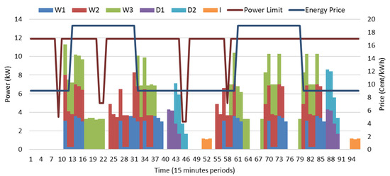
Figure 6.
Power consumption of devices in scenario C (based on double-tariff pricing and power consumption limit).
As it can be seen in Figure 6, the present method applies the power consumption limit on six periods and Figure 6 verifies that the optimization method has observed these limitations. These limitations are determinant in scheduling the device and they may force the consumption to be located at expensive periods.
For instance, Figure 6 presented that starting point of iron has been shifted from 53 to 50, and WM3 operation cycle in 55–60 has been shifted to 59–64 because of applied power limitation in 58.
Figure 7 shows the results of sensitivity analysis of power consumption limit in four levels as 90%, 95%, 105%, and 110% of the power consumption limit in scenario C.
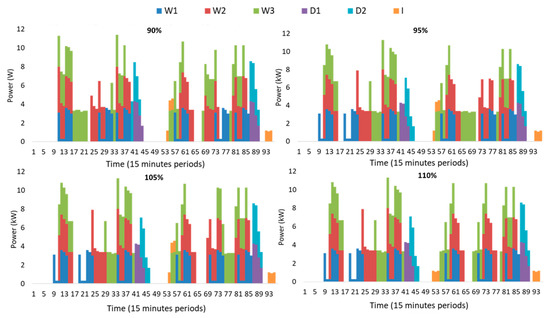
Figure 7.
Power consumption of devices regarding sensitivity analysis of power consumption limit.
According to Figure 7, it can be seen that small variations in power consumption limits have made several changes in the time of using the devices. The electricity cost calculation for each scenario can present the effectiveness of each variation.
Scenario D focuses on the implementation of the optimization method for 48 periods (1 day) instead of 96 periods (2 days). It should be noted that scenario D is based on double-tariff pricing and power consumption limit.
As it can be seen in Figure 8, the power consumption of iron has been shifted from the next day to period 46–48 of the same day. It shows that the iron could not be located in next day and this variation may affect the final electricity cost.

Figure 8.
Power consumption of devices in scenario D, focusing on 48 periods.
Figure 9 presents the scheduling of devices in scenario E based on the power consumption limit and dynamic tariff.
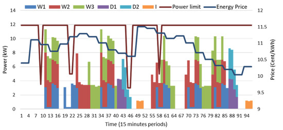
Figure 9.
Power consumption of devices in scenario E (based on dynamic tariff and power consumption limit).
According to comparison of first operation cycle of WM3 in scenario E and previous scenarios, the effect of dynamic tariff on load scheduling can be seen.
Figure 10 is related to scenario F to show the impact of incentives on the scheduling of devices. This scenario is based on dynamic-tariff pricing; however, 2 cents/kWh discount has been considered in periods 45–70 as an incentive.
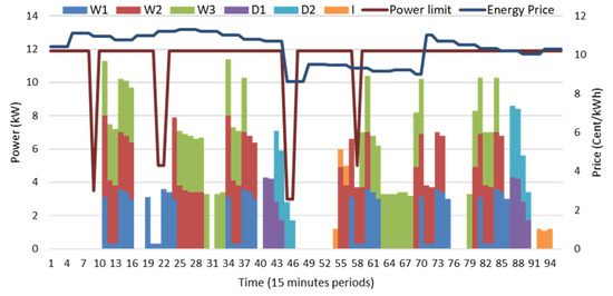
Figure 10.
Power consumption of devices in scenario F (considering incentive and power consumption limit).
As it can be seen in Figure 10, the starting point of the fifth operation cycle of WM3, has been shifted from 73 to 59 for taking advantages of applied discounts in these periods.
Figure 11 presents a general view of final power consumption in all scenarios.

Figure 11.
Total power consumption of devices in all scenarios.
In order to compare the efficiency of scenarios, Table 6 presents the energy cost in all scenarios. It should be mentioned that all ECs are shown as EUR/kWh.
Table 6.
Energy cost in all scenarios (SCN).
As it can be seen in Table 6, scenario A with a single tariff has the highest electricity cost. Scenario B has been decreased by 14.5 EUR/kWh from scenario A by applying a double tariff. Generally, scenario C shows that the power consumption limit has increased the cost. It means the power consumption of devices could not be shifted on off-peak prices in order to follow the limits. Scenario D shows that it is more efficient if the iron operates on the same day as WMs and dryers. EC in scenarios E and F show that dynamic tariff is cost-effective for consumers, however incentives in scenario F can compensate for the disadvantages of power limitation.
In order to compare the scenarios, it can be seen that scenario A was implemented for two days based on single-tariff pricing without any power consumption limitation. The user’s preferences such as the number of operations and time of operation were the important items for the methodology. The calculated electricity cost in scenario A was equal to 63.3 EUR/kWh. Scenario B was the same as scenario A in the context of the number of days, power limitations, and user preferences. However, the energy cost was based on double-tariff pricing. The energy cost in scenario B was calculated as 48.8. The comparison of scenario A and scenario B shows that the consumption pattern of the laundry room has been changed based on electricity price variations. Additionally, the electricity cost was reduced by 14.5 EUR/kWh in scenario B by double-tariff pricing.
Scenario C considered double-tariff pricing, power consumption limitation, and focused on two days. In fact, scenario C presented the effect of power limitation on energy consumption patterns. A sensitivity analysis in four levels was implemented for the power consumption limit. The obtained results of scenario C presented that power consumption limits can shift the power consumption of devices from rigid periods to free periods. However, the electricity price was increased compared to scenario B. This issue verifies the necessity of incentives for users in critical periods of the network.
Scenario D was implemented in one day, based on double-tariff pricing and the existence of power limitations was the same as in scenario C. In this scenario, ironing was not able to be postponed to the next day, and this difference changed the consumption pattern of the laundry room. The electricity cost presented for one day was equal to 25.4 EUR/kWh, which is lower than the electricity cost in scenario C.
Scenario E and scenario F were based on dynamic-tariff pricing. However, scenario F considered discounts in electricity cost as incentives. The calculated electricity cost in scenario E and scenario D were presented as 42.7 EUR/kWh and 40.9 EUR/kWh, respectively.
In addition to the monetary issues, user preferences and personal priorities are the important aspects that determine the efficiency of the method. For instance, scenario B is not the cost-effective one among scenarios, however, there is not any applied limitation for power consumption. In addition, scenario D seems more cost-effective compared to scenario C, however, the preference of the user about iron operation could not be achieved in scenario D.
The efficiency of the optimization methods depends on the flexibility of the users. It means that methods should take advantage of the flexibility of the users as much as possible, otherwise, those methods are not applicable for implementing in real life. In this way, the users can test different scenarios in order to obtain the best recommendation when the parameters from users are not well known or easy to define.
6. Conclusions
Demand response programs play an important role in the context of building energy management. They can manage the energy consumption pattern of users based on electricity price variations or other issues such as technical problems. In order to take advantage of demand response programs, buildings should be equipped with required infrastructures for running-related optimization methods. An optimization method has been proposed in this paper to optimize the energy cost of a laundry room equipped with three washing machines, two dryers, and one iron. This optimization method was based on different energy tariffs and observing the restrictions for power consumption. Additionally, the user’s preferences have been respected in the method such as the number of required operations for each device, time of operation of each device. For example, users have decided to postpone the iron operation to the next day. The purpose of the optimization method was to implement the load shifting based on different aspects. The sequence of operation of devices was an important item to increase the feasibility of the methodology. Six different scenarios were presented to show different outcomes of load schedule. The energy cost in all scenarios was presented in a table to compare the efficiency of scenarios.
As the main conclusion of this work, it can be seen that electricity price variation could take advantage of user flexibility in power consumption. It was clear that the total power consumption of users was not changed, however, the time of use was affected based on monetary benefits. Power consumption limitations may occur in an emergency situation of a network, however considering incentives for the user can increase the flexibility of the system. It was important to focus on the reliability of the method in the context of the sequence of operations and respect the user preferences in the methodology.
The proposed method can be integrated with renewable energy resources to implement the load shifting based on their power generation. In future works, authors are intended to propose the impacts of photovoltaic generation on load shifting. It means that load shifting should be implemented based on taking advantages of photovoltaic generation to minimize the cost.
Author Contributions
Conceptualization, P.F., Z.V., C.R.; Data curation, M.K.; Formal analysis, M.K.; Funding acquisition, P.F., Z.V.; Investigation, M.K., P.F.; Methodology, P.F., Z.V., C.R.; Project administration, P.F., Z.V., C.R.; Resources, P.F., Z.V.; Software, M.K.; Supervision, P.F., Z.V.; Validation, M.K., P.F., Z.V., C.R.; Visualization, M.K., P.F.; Writing—original draft, M.K.; Writing—review and editing, M.K., P.F., Z.V., C.R. All authors have read and agreed to the published version of the manuscript.
Funding
This work has received funding from Portugal 2020 under SPEAR project (NORTE-01-0247-FEDER-040224), in the scope of ITEA 3 SPEAR Project 16001 and from FEDER Funds through COMPETE program and from National Funds through (FCT) under the project UIDB/00760/2020, and CEECIND/02887/2017.
Conflicts of Interest
The authors declare no conflict of interest.
References
- Ascione, F.; Bianco, N.; Iovane, T.; Mauro, G.; Napolitano, D.; Ruggiano, A.; Viscido, L. A real industrial building: Modeling, calibration and Pareto optimization of energy retrofit. J. Build. Eng. 2020, 29, 101186. [Google Scholar] [CrossRef]
- Song, J.; Oh, S.; Song, S. Effect of increased building-integrated renewable energy on building energy portfolio and energy flows in an urban district of Korea. Energy 2019, 189, 116132. [Google Scholar] [CrossRef]
- Abrishambaf, O.; Lezama, F.; Faria, P.; Vale, Z. Towards transactive energy systems: An analysis on current trends. Energy Strategy Rev. 2019, 26, 100418. [Google Scholar] [CrossRef]
- Vural, G. Renewable and non-renewable energy-growth nexus: A panel data application for the selected Sub-Saharan African countries. Resour. Policy 2020, 65, 101568. [Google Scholar] [CrossRef]
- Khorram, M.; Faria, P.; Vale, Z. Optimizing Lighting in an Office for Demand Response Participation Considering User Preferences. In Proceedings of the 2019 International Conference on Smart Energy Systems and Technologies (SEST), Porto, Portugal, 9–11 September 2019. [Google Scholar]
- Alfaverh, F.; Denai, M.; Sun, Y. Demand Response Strategy Based on Reinforcement Learning and Fuzzy Reasoning for Home Energy Management. IEEE Access 2020, 8, 39310–39321. [Google Scholar] [CrossRef]
- Faria, P.; Barreto, R.; Vale, Z. Demand Response in Energy Communities Considering the Share of Photovoltaic Generation from Public Buildings. In Proceedings of the 2019 International Conference on Smart Energy Systems and Technologies (SEST), Porto, Portugal, 9–11 September 2019. [Google Scholar]
- Clairand, J.; Briceno-Leon, M.; Escriva-Escriva, G.; Pantaleo, A. Review of Energy Efficiency Technologies in the Food Industry: Trends, Barriers, and Opportunities. IEEE Access 2020, 8, 48015–48029. [Google Scholar] [CrossRef]
- Schwabeneder, D.; Fleischhacker, A.; Lettner, G.; Auer, H. Assessing the impact of load-shifting restrictions on profitability of load flexibilities. Appl. Energy 2019, 255, 113860. [Google Scholar] [CrossRef]
- Le, K.; Huang, M.; Wilson, C.; Shah, N.; Hewitt, N. Tariff-based load shifting for domestic cascade heat pump with enhanced system energy efficiency and reduced wind power curtailment. Appl. Energy 2020, 257, 113976. [Google Scholar] [CrossRef]
- Katz, J.; Andersen, F.; Morthorst, P. Load-shift incentives for household demand response: Evaluation of hourly dynamic pricing and rebate schemes in a wind-based electricity system. Energy 2016, 115, 1602–1616. [Google Scholar] [CrossRef]
- Beaudin, M.; Zareipour, H. Home energy management systems: A review of modelling and complexity. Renew. Sustain. Energy Rev. 2015, 45, 318–335. [Google Scholar] [CrossRef]
- Huang, G.; Yang, J.; Wei, C. Cost-Effective and Comfort-Aware Electricity Scheduling for Home Energy Management System. In Proceedings of the 2016 IEEE International Conferences on Big Data and Cloud Computing (BDCloud), Social Computing and Networking (SocialCom), Sustainable Computing and Communications (SustainCom) (BDCloud-SocialCom-SustainCom), Atlanta, GA, USA, 8–10 October 2016. [Google Scholar]
- Khorram, M.; Faria, P.; Abrishambaf, O.; Vale, Z. Consumption Optimization in an Office Building Considering Flexible Loads and User Comfort. Sensors 2020, 20, 593. [Google Scholar] [CrossRef] [PubMed]
- Jindal, A.; Singh, M.; Kumar, N. Consumption-Aware Data Analytical Demand Response Scheme for Peak Load Reduction in Smart Grid. IEEE Trans. Ind. Electron. 2018, 65, 8993–9004. [Google Scholar] [CrossRef]
- Khorram, M.; Abrishambaf, O.; Faria, P.; Vale, Z. Office building participation in demand response programs supported by intelligent lighting management. Energy Inform. 2018, 1, 9. [Google Scholar] [CrossRef]
- Wang, Y.; Tang, Y.; Xu, Y.; Xu, Y. A Distributed Control Scheme of Thermostatically Controlled Loads for the Building-Microgrid Community. IEEE Trans. Sustain. Energy 2020, 11, 350–360. [Google Scholar] [CrossRef]
- Wang, Y.; Xu, Y.; Tang, Y. Distributed aggregation control of grid-interactive smart buildings for power system frequency support. Appl. Energy 2019, 251, 113371. [Google Scholar] [CrossRef]
- Javaid, N.; Hafeez, G.; Iqbal, S.; Alrajeh, N.; Alabed, M.; Guizani, M. Energy Efficient Integration of Renewable Energy Sources in the Smart Grid for Demand Side Management. IEEE Access 2018, 6, 77077–77096. [Google Scholar] [CrossRef]
- Lynch, M.; Nolan, S.; Devine, M.; O’Malley, M. The impacts of demand response participation in capacity markets. Appl. Energy 2019, 250, 444–451. [Google Scholar] [CrossRef]
- Das, S.; Basu, M. Day-ahead optimal bidding strategy of microgrid with demand response program considering uncertainties and outages of renewable energy resources. Energy 2020, 190, 116441. [Google Scholar] [CrossRef]
- Khorram, M.; Faria, P.; Abrishambaf, O.; Vale, Z. Demand Response Implementation in an Optimization Based SCADA Model Under Real-Time Pricing Schemes. In Advances in Intelligent Systems and Computing; Springer: Cham, Switzerland, 2019; pp. 21–29. [Google Scholar]
- Khorram, M.; Faria, P.; Vale, Z. Load Shifting Implementation in a Laundry Room under Demand Response Program. In Proceedings of the 2020 International Conference on Environment and Electrical Engineering (EEEIC), Madrid, Spain, 9–12 June 2020. [Google Scholar]
- Krysiak, F.; Weigt, H. The Demand Side in Economic Models of Energy Markets: The Challenge of Representing Consumer Behavior. Front. Energy Res. 2015, 3, 24. [Google Scholar] [CrossRef]
- Teng, F.; Aunedi, M.; Pudjianto, D.; Strbac, G. Benefits of Demand-Side Response in Providing Frequency Response Service in the Future GB Power System. Front. Energy Res. 2015, 3, 36. [Google Scholar] [CrossRef]
- Ali, J.; Massucco, S.; Silvestro, F. Distribution Level Aggregator Platform for DSO Support—Integration of Storage, Demand Response, and Renewables. Front. Energy Res. 2019, 7, 36. [Google Scholar] [CrossRef]
- RStudio|Open Source & Professional Software for Data Science Teams. Available online: https://rstudio.com/ (accessed on 2 September 2020).


© 2020 by the authors. Licensee MDPI, Basel, Switzerland. This article is an open access article distributed under the terms and conditions of the Creative Commons Attribution (CC BY) license (http://creativecommons.org/licenses/by/4.0/).