Abstract
Industrial equipment such as electric arc furnaces and steel mills are often associated with rapid and high load disturbances, so their power systems require additional control equipment to limit the frequency. However, proper ancillary service fees are not paid in these cases with extreme and variable load demands. The frequency regulation reserve equipment adds to power generation costs. Therefore, variable power generation loads lead to increases in the cost of energy production. We propose a load frequency control method that is applied on the customer end instead of the power supply end to reduce the operating reserve required to improve the energy efficiency of the power system. We analyzed the load fluctuation of steel mill customers using real data sampled at two-second intervals from the energy management system in Korea. We developed an automatic generation control program to simulate the power system’s frequency characteristics. We also propose compensation techniques for mitigation of the system’s frequency deviation at the customer end based on an energy storage system, pump storage hydro generator, customer generator, and plant process adjustment. To recover the frequency deviation, we calculated the compensation facility capacity and analyzed static characteristics, and we proved the feasibility via simulations.
1. Introduction
Power system operator adjusts the schedule for power feeding to meet both the power demand and supply demand with the aim of managing power systems stably [1,2,3]. Generally, the demand forecasting for dispatch is based on one-hour estimations to facilitate planning of the generation schedule for the next day’s market. However, the power demand during the power system operation is fluctuated greatly by the short-period load variation within 1 h [4,5,6]. These intermittent load fluctuations may cause critical unbalance problems in operating power systems [7,8,9]. Therefore, the power system operator purchases ancillary service at a high price and provides such services for frequency following for the stabilization of power system [10,11].
The ancillary service is an indispensable function in terms of maintaining the quality of electricity. In addition, if this value added is not provided, it is impossible to maintain reliability by stabilizing the power system [12,13,14,15]. The ancillary service is the concept of power supply and demand regulation service, and there are services such as load following and energy imbalance as operation control to secure a supply and demand balance [14,15,16,17,18,19,20,21].
In South Korea, the power supply and demand of the Korea Electric Power Corporation (KEPCO) is based on the cost-based pool (CBP) for electric market systems. According to the procedure of daily demand estimation, the quantity of generation is determined using a demand estimation system. More specifically, power generation bidding is carried out according to the estimated power demand every hour for a total of 34 h, comprising 6 h before the transaction for generation planning, 24 h for the date of transaction, and 4 h after the transaction. However, because of the large and short-term fluctuations, which exceed the contracted capacity of the demand meter (DM), the loads of the steel manufacturing industry have a serious effect on the 1 h-based power supply system [22].
The current real-time power system operation calculates the power demand using the energy management system (EMS)’s 5-min demand forecasting program, and the economic load dispatch (EDC) program calculates and orders the generation of each generator to cope with short-term power demand. In other words, to cope with power demand and supply, the frequency regulation reserve against load fluctuation is expanded. However excessive frequency regulation reserve expands the control range of automatic generation control (AGC) and governor free (GF) control for generators, which in turn leads to the low efficiency generator operation and an increase in fatigue in turbine and steam systems, thereby increasing the frequency of system failures. As a result, power generation cost increases and system reliability declines. Nevertheless, there is no regulation in South Korea for those who cause specific ancillary service operations and frequency deviations in power systems. Therefore, some customers, such as companies with electric arc furnaces and steel mills, have highly variable electric load demands, but do not pay proper ancillary service fees for them. The total power system management cost is shared between those who impose extreme load demands and general users. Steel manufacturing establishments in South Korea typically have their own generators and generate power using gas by-products. Nevertheless, they generate power at a fixed maximum rate and sell it back to the Korea Electric Power Corporation (KEPCO) utility because the rate charged for electricity production via gas by-products is far greater than that of the electricity supplied by KEPCO. Therefore, it is important to impose reasonable fees to better cope with the situation.
Load frequency fluctuation has been of interest for decades with the aim of increasing the power system’s stability and assessing fair electricity usage fees [23,24,25]. Recently, the issue has emerged as a research topic because of the intermittent renewable energy resources penetrating the grid. The IEEJ has studied load variation characteristics, frequency regulation effects, and control methods [26,27]. The Department of Energy analyzed the frequency fluctuation caused by a wind turbine using the spectrum method and reviewed the use of an energy storage system (ESS) for power balancing [6,16,28]. Kirby discussed the economical effectiveness of “causer pay” for ancillary services and the principle of fair benefit sharing [12]. Wolak suggested a payment mechanism for ancillary services for the Chilean electricity supply industry [29]. Chu and Chen proposed a cost allocation strategy for primary frequency regulation (PFR) services at the customer end [30]. Shoults et al. developed area control error (ACE) filtering techniques and load frequency control (LFC) logic to address the AGC performance problem attributed to arc furnace steel mill loads [31]. However, no other research has been performed on load-following generator operation at the customer end.
Most studies have focused on frequency control at the supply end, but in this study, we focused on the customer end. We analyzed the load fluctuation caused by steel mill customers using real data sampled at two-second intervals obtained from the energy management system (EMS) in Korea. We then developed an AGC program to simulate the frequency characteristics of the power system. Additionally, we discuss compensation equipment and techniques to mitigate the system’s frequency deviation at the customer end. These include an ESS, pump storage hydro-generators, customer generators, and plant process adjustment. The effects of the compensation equipment were analyzed.
The remainder of this paper is organized as follows. Section 2 describes our analysis of the load fluctuation caused by steel mill customers. Section 3 introduces the AGC program, and Section 4 presents our analysis of the frequency deviation characteristics of a power system for steel mill load. In Section 5, we discuss the simulation of the proposed measures to mitigate load fluctuation, and we conclude the paper in Section 6.
2. Analysis of Load Fluctuation of a Steel Mill
2.1. Korean Operating Reserves
Ancillary services are important for ensuring that targeted objectives are fulfilled for a power system’s security, frequency stability, voltage level, and voltage stability. Operating reserve is an important type of ancillary service that supports system reliability in the face of unexpected generator outages. Table 1 shows the operating power system reserves in Korea. An operating reserve is composed of regulating and supplemental reserves. A regulating reserve, corresponding to the frequency-response reserve, provides ancillary services through governor-free (GF) control and an AGC to maintain real-time balance in the system and frequency control. The size of the reserve amounts to 1500 [MW].

Table 1.
Operating reserves in Korea.
The supplemental reserve consists of operational and standby reserves, and the operational condition corresponds to power being generated that is already synchronized with the ISO controlled grid. The reserve is 1000 [MW] under normal operation and 1500 [MW] in an emergency. The allocated reserve for standby conditions is 1500 [MW] under normal operation and 1000 [MW] in winter and summer.
The spinning reserve [32] corresponds to the sum of the regulating reserve and supplemental reserve. During operation, this reserve is 2500 [MW]. The non-spinning reserve is 1500 [MW]. The peak demand in 2013 was approximately 76.5 [GW], and the spinning reserve accounted for 3.1% of the peak load.
2.2. Load Fluctuation of Steel Mills in Korea
The daily load curves of the total power system and the steel manufacturing industries in winter, spring and summer are shown in Figure 1a,b, respectively. This load data is recorded every 2 s from the EMS. The load curve of the total power system shows an accumulated load characteristic due to the overlap of the various loads.
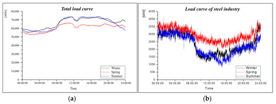
Figure 1.
The daily load curves in South Korea: (a) Load curves of total power system; (b) Daily load curves of all steel mill customers.
The variable loads have similar patterns for hourly, daily, weekly, monthly, and yearly periods, but patterns may become more random due to the fluctuating demand loads of industry and increasing environmental effects and human behavior. The smaller number of demand loads has a noisy cyclic complex curve while the larger number of loads has a fairly smooth curve. However, the fluctuation of the total demand load in the power system depends on that of the combination of individual loads.
Due to increased heater and air conditioning loads in winter and summer, the load demand is higher than that in the spring. If the individual load is separated from the total overlap load, the short-term load fluctuation appears to be serious. In particular, the load fluctuation for the steel manufacturing industry appears to be large, as shown in Figure 1b. This is caused by the instantaneous operation of many different facilities used for arc furnace, rolling, etc. This load curve shows a similar pattern in winter and summer. On the other hand, during the daytime in spring, the load curve shows a high power consumption pattern. Figure 1b shows higher power consumption at daytime in spring than winter and summer, and at night time than during daytime in winter and summer, because demand side management (DSM) is carried out by time-of-use (TOU) pricing. The TOU standard of Korea is classified according to the season and time. Typically, the load levels are divided into three levels: light load level (23:00–09:00), heavy load level (09:00–10:00, 12:00–13:00, 17:00–23:00), and peak load level (10:00–12:00, 13:00–17:00).
If the daily load data in Figure 1 is analyzed by time period, the results show that various cycle components are combined, as shown in Figure 2. To analyze such cycle components, a frequency band analysis method based on weighted moving average (W-MA) and a method for calculating the spectrum density by way of fast Fourier transformation (FFT) coding of the auto-correlation function are used [33,34,35,36,37]. The results of these two different methods are known to be almost the same.
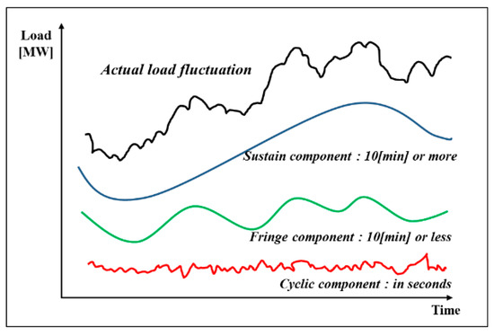
Figure 2.
Periodic component of load fluctuation.
The correlation between the spectrum density (SL(ω)) and angular frequency (ω) is shown as Equation (1). Disturbance has a different cycle depending on time. The results show a 15 min cycle standard deviation of disturbance, which is almost proportional to the square root of the system capacity, as shown in Equation (2).
- SL(ω): Magnitude of the disturbance (Spectral density [MW2·sec]);
- A: Proportional constant;
- ω: Angular frequency of the disturbance;
The value of ‘n’ is about ‘1’.
- σD: Standard deviation of the disturbance (MW);
- P: System capacity;
- γ: Proportional constant.
To analyze the load variability, the authors analyzed the frequency spectrum of the steel manufacturing load using FFT. If the daily load data is analyzed by spectrum analysis using FFT, the results show the characteristics of the frequency band, as shown in Figure 3.
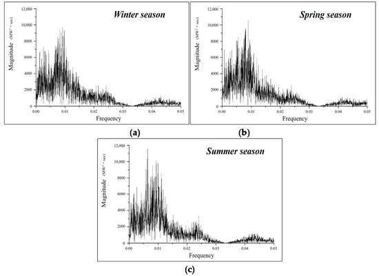
Figure 3.
Frequency spectrum of fluctuation for total steel industrial loads: (a) Winter season; (b) Spring season; (c) Summer season.
Table 2 shows the correlation between the frequency band and the load fluctuation time.
Table 2.
Frequency bands for the period of load fluctuation.
If we assume that the disturbance analyzed has a normal distribution, it can be presented as shown in Figure 4.
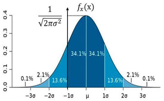
Figure 4.
Distribution curve about statistics.
- X: Random variables;
- μ: Average data;
- σ2: Fluctuation data.
The distribution of the load fluctuation components is shown as the range of size of fluctuation components, and this can be shown by the range of standard deviation. Regarding the standard deviation adopted in this study, the variability of 2σ with a probability of 95.44% was used as the acceptable load fluctuation, so as to ensure compatibility. Table 3 shows the data distribution percentage. σ shows the probability of exceeding the data range, and the 3σ regulation implies that the range of σ standard deviations from the mean includes almost every value (99.7%). Standard deviation analyzes the difference between the size of each load fluctuation and the mean fluctuation, while the statistics are reported as means, thus providing the distribution of load fluctuation.
Table 3.
Probability value corresponding of the data ratio.
In this paper, we calculated the load increase rate considering the load forecasting component, and this is used in the moving average (MA) method. The load fluctuation data with respect to time period is obtained by comparing the MA data with the increasing rate data.
The statistical equations to analyze the size of average load and load fluctuation are shown as Equations (4)–(7). The mean load capacity is calculated to analyze the range of load fluctuation, and the equation for calculating the mean is shown in Equation (4). Equation (4) is used to calculate the growth rate of the load capacity and the size of the load fluctuation, as shown in Equation (5). With respect to the temporal means, the size of load fluctuation is calculated using the difference between average load and load growth rate, and the load fluctuation for average load time can be calculated using Equation (6).
The distribution curve of load fluctuation was calculated using the equation for calculating standard deviation, Equation (7), where N is load average time and I is the size of real-time load fluctuation.
where ‘N’ is average time of load, and ‘i’ is the real-time load fluctuation value.
Table 4 shows the calculation criteria for load fluctuations using the moving average method presented in this paper. We calculated the MA for the time period, and calculated the MA increase rate for 1 h, 10 min, and 30 s. The calculation of load fluctuation magnitude with an average time of 15 min was based on the average increase rate of 1 h. The calculation for fluctuation magnitude for average times of 10, 5 and 1 min were based on an average increase rate of 10 min, and the rest were based on the 30 s increase rate.
Table 4.
Calculation of the load fluctuation magnitude about MA.
By using the load variability analysis method proposed, the size of load fluctuation in the daily load data can be determined for the steel manufacturing industry, major steel manufacturers, and representative steel manufactures. The magnitudes of load fluctuation for the total steel industry according to the load levels and the seasons are shown in Table 5.
Table 5.
The load fluctuation magnitude of total steel industrial.
3. AGC Program
PSS/E can simulate a power system’s transient effects for only a few seconds, so we developed an AGC program called KEPCO Automatic Generation Control (K-AGC) to simulate the power system load fluctuation for longer than 10 min [38,39]. This program is composed of a text viewer, load-flow calculation, and AGC simulation and can simulate both the transient and steady-state behavior of a power system. Figure 5 shows a block diagram of the K-AGC program. It can accommodate several areas to configure a power system. Figure 6 shows the AGC configuration. One area is composed of SYS, LOAD, economic dispatch control (EDC), and ACE. SYS is a damping constant that represents the frequency characteristics for a difference between the generation and zone load, and LOAD is the load fluctuation for the frequency deviation. The AGC is executed for each zone, and every zone is connected to other zones by tie lines.
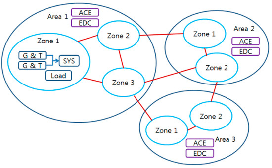
Figure 5.
Block diagram of K-AGC.
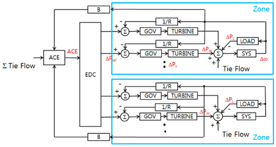
Figure 6.
AGC configuration.
Figure 7a shows a flow chart of the steady-state analysis. The program can calculate the frequency deviation for a load change and the load deviation for a frequency change. There are two modes in the steady-state analysis: governor-lock (GL) and GF modes. The GL mode considers only the load coefficient (KL), but the GF mode considers the generator coefficient (KG) and KL.
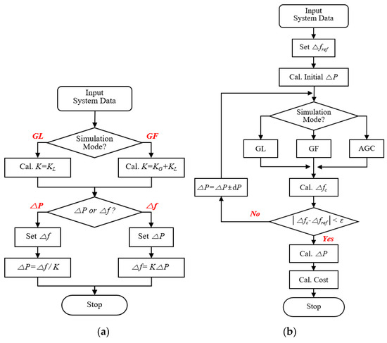
Figure 7.
Flow chart of steady-state and transient-state analysis: (a) Steady-state analysis; (b) Transient-state analysis.
Figure 7b shows a flow chart for the transient-state analysis, which has three modes: GL, GF, and AGC. The procedure for LFC is summarized as follows:
Figure 8 shows the developed AGC program. The text-based input window of Figure 8a is for the input of system model and initial data, and the execution window of Figure 8b is for the calculation of the size of load fluctuation and the results of frequency deviation.
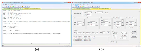
Figure 8.
Developed AGC program: (a) Input tab of the model data; (b) Tab of the set and run.
- Step 1: Input power system data;
- Step 2: Set the reference frequency deviation;
- Step 3: Calculate initial load deviation;
- Step 4: Select simulation mode from among GL, GF, and AGC modes;
- Step 5: Calculate frequency deviation and determine whether frequency error is within the tolerance. If the error is less than the tolerance, go to step 6. Else increase/decrease load deviation by dP and go to step 4;
- Step 6: determine load deviation and calculate cost for ancillary service.
We analyzed the results using the 1-bus stand-alone model and the data in Table 6 to confirm the reliability of the developed AGC program. As shown in Figure 9, the frequency deviation characteristics for the 500 [MW] load fluctuation at 10 s were the same as the PSS/E (version 33.4.0 SIEMENS PTI) results. The AGC program’s accuracy and reliability were verified by comparing the calculation results with those of PSS/E [40].
Table 6.
The simulation data of grid-connected system.
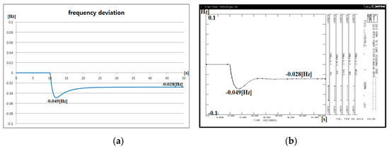
Figure 9.
The frequency characteristic of grid-connected system: (a) Results of the AGC Program; (b) Results of PSS/E.
4. An Analysis of Frequency Characteristics
In this paper, we conducted a simulation by dividing the model into a single model and a network model according to the connections between generators and loads, as shown in Figure 10. In addition, this model is divided into a single capacity system for individual companies, a business type capacity system, and a total system capacity system. The single model considers the generators owned by individual companies and the characteristics of the steel manufacturing load. The generators owned by the companies in Zone 2 of the single model are based on a locked output. With respect to the network model, Load_b in Figure 10b shows the steel manufacturing load, and Load_a shows the total load of the power system excluding the steel manufacturing load. Zone 1 comprises generation data and general load data and Zone 2 comprises steel load data, fluctuation data and the data of the generators owned by companies.
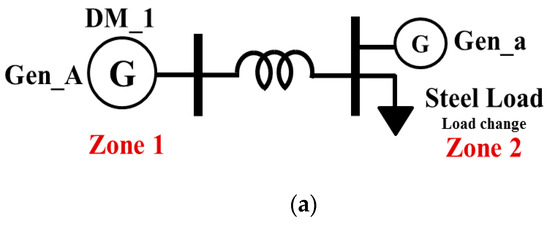
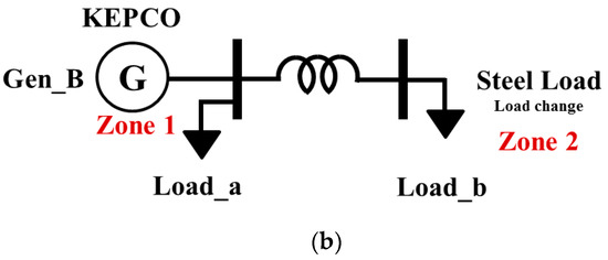
Figure 10.
Model for simulation: (a) 1-bus stand-alone model; (b) 1-bus network model.
In a simulation model, the susceptance of the tie line, the maximum power demand, the load level, the reserve, and the self-generation capacity data are needed.
The inertia coefficient of the generators was calculated as 4.85 using Equation (8).
- Mi: Inertia coefficient of the generator;
- Pi: Capacity of the generator;
- Ptotal: Total capacity of the generator.
Regarding the susceptance of the tie line, the fault capacity was calculated using load flow data, and Thevenin’s equivalent impedance for the respective bus was used. The susceptance of the tie line for steel company P was 0.00096 + j0.00578 [Ω], and the susceptance of the tie line for the load of all the steel companies was 00020 + j0.00159 [Ω].
The reserve value was calculated on the basis of the maximum power demand of 74,000 [MW] in summer (2013.08). More specifically, stand-by/replacement reserve (operation state) values of 2500 [MW] (spring and fall season) and 3000 [MW] (winter and summer season), including a frequency regulating reserve of 1500 [MW], were calculated proportionally.
This implies that the reserve model is calculated by the proportion to the maximum demand, and the frequency regulating reserve () has a value of 2.03%, and the stand-by/replacement reserve () has a value of 3.38% (spring and fall season) and 4.05% (winter, summer season).
To analyze the frequency characteristics of load fluctuation, the load fluctuation was divided into season, load level and load capacity.
In general, with respect to response speed, GF operation is fastest, followed by AGC operation. Thus, to analyze the frequency characteristics, integrated times of 10 and 30 s were applied to GF operation, and integrated times of 60, 300, 600 and 900 s were applied to AGC operation.
In this paper, to show the frequency deviation distribution, the frequency deviation of a steady-state power system within 0.2 [Hz] was defined as [State I], the operation frequency of under frequency relay (UFR) within 3.0 [Hz] was defined as [State II], and the rest was defined as [State III].
4.1. An Analysis of the Single Capacity Model
To analyze the single capacity model, we used the load fluctuation data in Table 5, the single model in Figure 10a, and the simulated reference data in Table 7.
Table 7.
Simulation data of the P steel company.
The characteristics of dynamic frequency of representative steel manufacturer (P company) is shown in Figure 11. In a few typical cases, Figure 11 shows frequency characteristics for the magnitude of load fluctuation within the reserve and outside the reserve. As shown in Figure 11a, the magnitude of load fluctuation is within the frequency regulating reserve, so the frequency deviation is stable within −0.0542 [Hz]. However, the magnitude of load fluctuation is outside the reserve in Figure 11b, so the frequency regulating reserve is insufficient; thus, the frequency characteristics of the generator were not reflected. As a result, the frequency deviation was as significant as −2.975 [Hz]. In Figure 11c, the magnitude of load fluctuation is within the stand-by/replacement reserve, and the frequency deviation is recovered to 60.0 [Hz]. However in Figure 11d, the magnitude of the frequency deviation is outside the stand-by/replacement reserve, so the frequency is not recovered. Outside the limits of the reserve, the frequency characteristics of the power system do not reflect the characteristics of generation power-frequency. In other words, the results depend on the frequency characteristics of the load. The frequency deviation distribution of a steel manufacturing company P is shown in Figure 12. [State I] is 5.8%, [state II] is 83.3%, and [state III] is 1.9%. The frequency deviation in [State II] is the greatest.
Figure 11.
Frequency deviation of the load fluctuation (P company, summer season): (a) GF response characteristics (light load 10 s-1σ); (b) GF response characteristics (peak load 30 s-3σ); (c) AGC response characteristics (light load 900 s-1σ); (d) AGC response characteristics (light load 600 s-3σ).
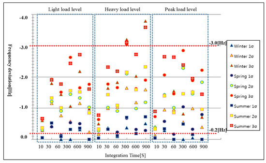
Figure 12.
Frequency deviation distribution chart of P company (single model).
4.2. An Analysis of the Business Type Capacity Model
We grouped Korea’s leading steel manufacturing companies, P, K and H, together and analyzed their frequency characteristics in conjunction with load fluctuation. To this end, we used the load fluctuation data in Table 5, the single model in Figure 10a, and the simulated reference data in Table 8.
Table 8.
Simulation data of the group of steel companies.
The dynamic frequency characteristics for business type capacity are shown in Figure 13. The magnitude of load fluctuation exceeds the frequency regulating reserve and stand-by/replacement reserve in Figure 13b,d, showing significant frequency deviation. The distribution of the frequency deviation for the load fluctuation of major business types is shown in Figure 14. [State I] was 29.6%, [State II] was 66.0% and [State III] was 4.4%, showing that [State II] has the greatest frequency deviation. Since the business type model has a greater reserve and a higher load level than the single capacity model, the ratio of [State I] is higher and the frequency deviation is, in general, lower.
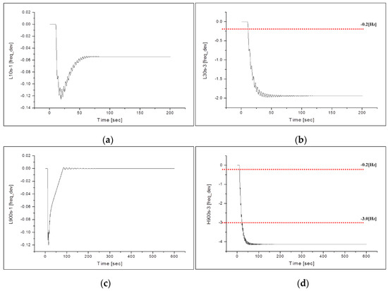
Figure 13.
Frequency deviation of the load fluctuation (steel company group, summer): (a) GF response characteristics (light load 10 s-1σ); (b) GF response characteristics (light load 30 s-3σ); (c) AGC response characteristics (light load 900 s-1σ); (d) AGC response characteristics (heavy load 900 s-3σ).
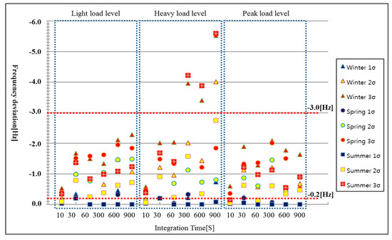
Figure 14.
Frequency deviation distribution chart of the group of companies (business model).
4.3. An Analysis of the Network Connected Model
We analyzed the frequency characteristics of the power systems for the load fluctuation of whole domestic steel manufacturing companies. To analyze the network model, we used the load fluctuation data in Table 5, the network model in Figure 10b, and the simulated reference data in Table 9.
Table 9.
Simulation data of the whole company.
The dynamic frequency characteristics of the network model are shown in Figure 15. Since the magnitude of load fluctuation in whole steel manufacturing companies is within the range of the stand-by/replacement reserve, the frequency deviation was low, showing a stable state. In addition, the frequency deviation distribution in Figure 16 shows a [State I] ratio of 100%. This implies that, as there is sufficient reserve that is capable of supporting the variability in the loads of whole steel manufacturing companies, the frequency deviation is within 0.2 [Hz], or all can be recovered to 60 [Hz].
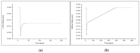
Figure 15.
Frequency deviation of the load fluctuation (all steel company, summer): (a) GF responsive characteristics (light load 10 s-3σ); (b) AGC responsive characteristics (heavy load 600 s-3σ).
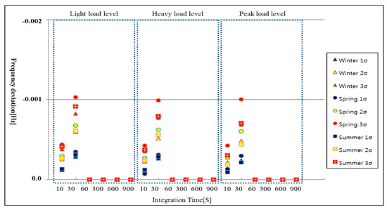
Figure 16.
Frequency deviation distribution chart of all steel company (network model).
4.4. The Results of Frequency Deviation Analysis
The frequency deviation distributions of the single capacity model, the business type model, and the network model analyzed in this paper are shown in Figure 17. If the frequency deviation characteristics of companies P, K and H are compared with the those of the business type model and the network model, the frequency deviations gradually decrease. This is because the business type model and the network model have greater characteristics of generation power-frequency and load-frequency than the single capacity model. In other words, as the load level and reserve increase, the frequency deviation for load fluctuation decreases.
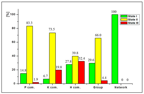
Figure 17.
Analysis of the frequency deviation range.
5. Frequency Deviation Analysis of a Power System with Compensator
The power system control block diagram consists of an inertia generator, damping coefficient, and governor characteristics [1]. We analyzed the frequency deviation characteristics with load fluctuation by adding a model of a compensation facility, as shown in Figure 18 [38,39,41]. To determine the frequency deviation, the compensation facility capacity was calculated, and the static characteristics were analyzed. The transfer function between the load fluctuation and frequency deviation of a power system without a compensator is represented by Equation (9), where M is a momentum constant, D is the load damping, and is the governor characteristic:
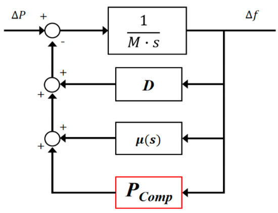
Figure 18.
Block diagram of power system with compensator.
LFC with a compensation facility with characteristic constant is represented Equation (10), where is the improved compensator frequency deviation:
To be considered a steady-state frequency () in Korea, the improved frequency deviation should be within ±0.2 [Hz]. Thus, the minimum compensation facility’s capacity for the improved frequency to become a steady-state frequency is:
where the characteristic constant of the compensation facility is:
Equation (12) represents a case where load fluctuation occurs within the spinning reserve range considering speed droop and load damping.
When the load fluctuation exceeds the governor’s operating range, the frequency deviation characteristics are proportional to the compensation facility capacity, as shown in Equations (13) and (14):
where is the spinning reserve capacity of the governor. By substituting the compensation model into Equation (14), the compensated characteristic equation for the control system is obtained:
The compensation capacity equation for steady-state frequency () operation is:
where () is the frequency regulation reserve divided by each generator due to the limitations of the governor response. Figure 19 shows the compensation capacity and slope for steady-state frequency deviation caused by load fluctuation.
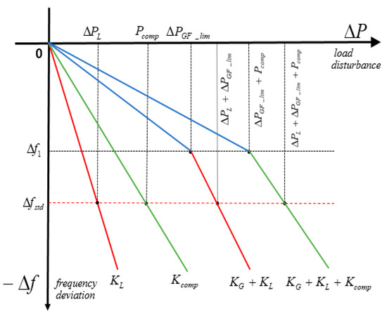
Figure 19.
Slope and compensation capacity with frequency deviation.
5.1. Compensator Model and Characteristics
5.1.1. Compensator Characteristics
In this paper, we selected the following compensator models for load fluctuation mitigation: an ESS, a peak reduction (PR) generator, and a customer-owned (CO) generator. The compensator model is based on the IEEE model, the ESS is a battery-based BESS1 model, the PR generator is the GOVHYD model, and the CO generator is the IEEEG1 model. Equations (17)–(19) represent the mathematical models of each compensator.
As the speed droop of each compensator, 1% for BESS, 3% for GOVHYD, and 5% for IEEEG1 are applied, and then summarized as an equation for the frequency deviation, as shown in Equations (20)–(22).
An independent ACE model was constructed as shown in Figure 20 to analyze the PFR characteristics of each model of the compensator. The system inertia of the power system was ‘10’ and a load damping of ‘3’ was applied. The governor and turbine models compared and analyzed the characteristics of the 10 [MW] load fluctuation at 5 s under non load-following conditions.
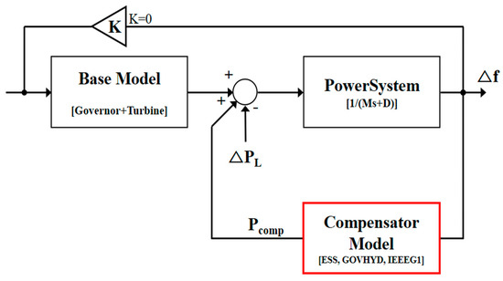
Figure 20.
Configuration for simulation of compensation equipment.
Figure 21 shows the frequency characteristics of each compensator, and the response characteristics of ESS are the fastest, so it is very effective in PFR, and its value as an ancillary service is very high. However, due to its shorter duration, lower capacity and higher cost compared to other compensators, appropriate choices are needed.
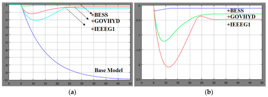
Figure 21.
The frequency characteristics of each compensation equipment: (a) Compensation facility characteristics; (b) Compensator characteristics.
5.1.2. Improved Compensator Control Method
The control block diagram for the PFR improvement method is shown in Figure 22, and the compensation coefficient setting by frequency deviation is applied to each compensator. The characteristics are analyzed as the self-tuning value with respect to frequency deviation proportionality.
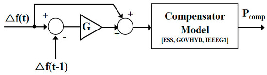
Figure 22.
Improved method by Primary Frequency Regulation.
For the characteristics analysis of the improved control method, the characteristics of the compensators were analyzed by applying the frequency error gain value under the same conditions as the configuration diagram in Figure 22. We applied gains values of ‘1’, ‘2.4’ and ‘3.2’ for BESS, ‘1’, ‘18’, ‘24’, for GOVHYD, and ‘1’, ‘15’, and ‘48’ for IEEEG1 as the error correction factors for each compensator, and the frequency characteristics are shown in Figure 23.
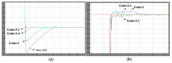
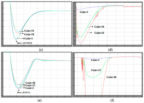
Figure 23.
The frequency characteristics for an improved method: BESS frequency characteristics; (a) BESS frequency characteristics; (b) BESS error correction characteristics; (c) GOVHYD frequency characteristics; (d) GOVHYD error correction characteristics; (e) IEEEG1 frequency characteristics; (f) IEEEG1 error correction characteristics.
When a frequency deviation occurs due to load fluctuations, since the output of the governor is controlled by the difference from the reference frequency, the improved control method with an error correction factor has a lower frequency deviation of the PFR term and a higher recovery speed than the conventional control method. The larger the frequency error correction factor, the faster the recovery speed of the PFR, but as the self-excited vibration (oscillation) occurs after non-ideal control and frequency recovery exceeding the system maximum response speed of each compensator, a correction factor must be set for the system response characteristics.
5.2. Case Study
We propose four ways in which steel mills can execute the LFC: an ESS, a PR generator, GF operation of a CO generator, and changing industry processes to mitigate load fluctuation. Additionally, we investigated the frequency impact of a load change using a single bus model for four cases. We used an independent power system model to simulate the four proposed measures, as shown in Figure 24. We assumed that the power system generator is in a governor lock condition (load limit), and that the demand end is connected to a compensation facility that is capable of GF and AGC. In this paper, the generator capacity of the system is the same as the contracted power of the load, and the governor operating range corresponding to the frequency adjustment reserve is allocated to the generator. The load is selected as the most frequent value of the average power in units of 5 min for each time period of the intermittent load, and the frequency deviation characteristic is simulated by inputting the load fluctuation magnitude.
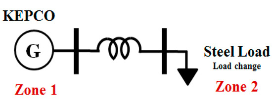
Figure 24.
Simulation model.
The simulation data are shown in Table 10. %R is 5% MW/Hz, and %D is 3% MW/Hz. The 1st operating reserve is 14.01 [MW], and the 2nd operating reserve is 27.95 [MW], which are proportionally allocated according to each generator’s capacity and correspond to GF and AGC operation, respectively.
Table 10.
Simulation data for steel mill B (winter, light load).
5.2.1. Addition of ESS
An ESS is used for various purposes, such as load shifting, peak shaving, smoothing of photovoltaic and wind turbine output, and frequency regulation. The duration of the ESS reserve operation is shorter than that of the generator, but the load following speed is faster, so we can use the ESS as a reserve resource. We adopted an ESS for frequency regulation to control the frequency deviation caused by mill-load fluctuation. Figure 25 shows the power system simulation model with an ESS for facility compensation.
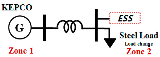
Figure 25.
Power system model with ESS.
We used a 30-s 3-sigma average load variation from steel mill customer B, which is a 147 [MW] increase. We assumed that the 1st reserve was 14.01 [MW] and that the output power of the CO generator was fixed at 900 [MW]. The speed droop in this case was 1%. In this simulation, we analyzed the effect of the ESS during 3 min after the load fluctuation before the AGC operation. According to Table 10, the primary reserve power is 14.01 [MW], and the load fluctuation amount 132.99 [MW], obtained by subtracting the reserve power from the load fluctuation magnitude of 147 [MW] causes a frequency deviation due to the load frequency characteristics. Thus, the ESS capacity for maintaining frequency within 0.1 [Hz] can be calculated using Equation (3), as shown in Equation (23). The rest is covered by the 1st reserve and load damping.
Figure 26 shows the simulation output obtained with and without the ESS. Without the ESS, the results show a frequency deviation of 3.1 [Hz] due to a lack of operational reserves. The deviation is only 0.1 [Hz] for the model with the ESS, and the frequency response time is less than one minute. The ESS is very effective for fast load-following operation.
Figure 26.
Output analysis of ESS added system: (a) Frequency characteristics; (b) ESS power output.
5.2.2. GF Operation of a Customer-Owned Generator
In the next case, we assumed that a customer-owned generator was used for the LFC, as shown in Figure 27. We simulated two cases: one for GF operation and another for AGC operation, including the GF mode. The speed droop in this case was 5%.The given data are as follows: a load fluctuation of 219.5 [MW] (10-min 3-sigma fluctuation in the winter season) and a 2nd operating reserve of 27.95 [MW]. The 2nd reserve required for AGC operation is 191.55 [MW] with 27.95 [MW] subtracted from the entire load fluctuation.
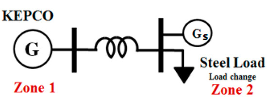
Figure 27.
Power system model with customer-owned generator.
Figure 28 shows the simulation results for the load-following customer-owned generator operation. The resulting frequency deviation was −4.49 [Hz] for fixed output operation, −0.333 [Hz] for GF mode, and 0.0 [Hz] for GF/AGC mode. Additional power output of 177.4 [MW] and 191.6 [MW] is needed for GF and GF/AGC modes, respectively.
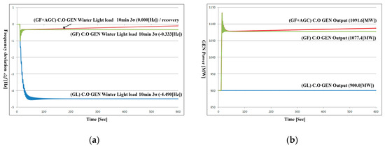
Figure 28.
Output analysis when a customer-owned (CO) generator is used for frequency regulation: (a) Frequency characteristics; (b) Generator power output.
5.2.3. Addition of Peak Reduction Generator
A Diesel generator and hydroelectric generator can be used for peak reduction. We considered a hydroelectric generator as a compensation facility to mitigate the load fluctuation. For peak reduction in this case, we used two hydroelectric generators with 100 [MW]. The generator is denoted by Gp in Figure 29, which has a 3% droop rate. The assumed load variation was a 155.5 [MW] increase, which was a 5-min 3-sigma fluctuation during light-load operation of the power system. The 2nd reserve was 27.95 [MW], and the customer-owned generator power output was fixed at 900 [MW]. We analyzed the frequency response for the three cases during 10 min of operation: (i) without Gp, (ii) GF operation with Gp only, and (iii) GF + AGC operation with Gp.
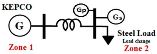
Figure 29.
Power system model with a PR generator, labeled as Gp.
Figure 30 illustrates the simulation output for the PR generator case. Without PR generators, the results show a frequency deviation of 2.99 [Hz] due to the lack of power supply. The GF-limited operation using two hydroelectric generators has a frequency deviation of 0.83 [Hz], and the output contribution of the PR generators is 92.16 [MW]. For case (c), the output increases to 126.97 [MW], and the frequency stabilizes without deviation. The results show that using a PR generator is an effective way for LFC to stabilize the frequency within 10 min.
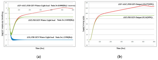
Figure 30.
Output of system with PR generator: (a) Frequency characteristics; (b) PR generator power output.
5.2.4. Change of Industry Processes
The load fluctuation caused by a steel mill can be improved by adjusting the manufacturing process without decreasing productivity through load re-distribution and re-allocation. Load re-distribution is the equalization of load changes by adjusting all other mill processes except the essential processes. In other words, it is the same as the method of leveling the load through peak-cut. In the case of a process with large load fluctuations, it is a method of improving the process by reducing the use of other loads and making the magnitude of the load fluctuation constant. In addition, load re-allocation is the alteration of the process sequence according to the power system demand or factory load level. In this case, the process is changed according to the daily load level. However, although theoretical proposals are possible, there are difficulties in practical application. We simulated three cases of process changes, as shown in Table 11. Case 1 is for the original process, case 2 is for load re-distribution, and case 3 is for load re-allocation.
Table 11.
Simulation cases.
For each case, three kinds of load variances were added for 10 s while linearly increasing the load by 100 [MW] for 30 s. Figure 31 shows the simulation input profiles for these 3 cases. In Figure 31a, there is a step change of 21 [MW] at time zero, 75 [MW] at 10 s, and 131.5 [MW] at 20 s, which lasted for 10 s each. A similar method was used for cases 2 and 3.
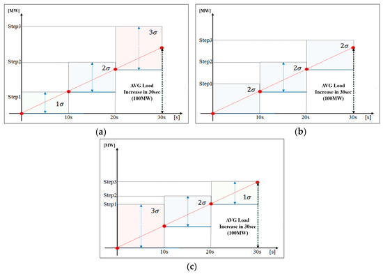
Figure 31.
Simulation profile for process change: (a) Original process; (b) Load re-distribution; (c) Load re-allocation.
Figure 32 shows the transient simulation results for the process change. Figure 32a shows that the frequency deviations at steady state are 2.76, 2.24, and 1.73 [Hz] for cases 1, 2, and 3, respectively. Rearranging the process to decrease the load fluctuation magnitude over time resulted in a better frequency response with respect to the operational reserve.
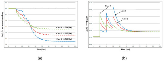
Figure 32.
Simulation output for process change: (a) Frequency characteristics; (b) Load characteristics.
Figure 33 summarizes the mitigation effects of the simulation results. We can improve the frequency deviation response by 30% just by changing the process sequence without any extra investment. The frequency deviation is recovered within one minute when using the ESS, 5 min when using the pump storage hydro-generator, and 10 min when using the customer’s generator.
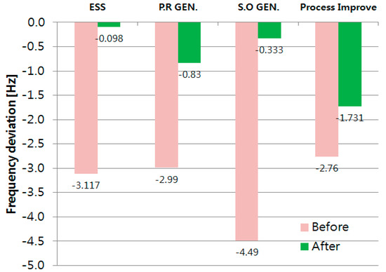
Figure 33.
Comparison of simulation results.
6. Conclusions
In this study, we analyzed the effect of the variability of large-scale industrial load on the frequency of power systems and the load fluctuation frequency spectrum of the steel manufacturing industry, showing substantial load fluctuation, time zones where load fluctuation occurs, and the magnitude of load fluctuation. In addition, we analyzed the frequency characteristics using the EMS (Energy Management System) real-time data when powering systems including steel mills, resulting in customers with three kinds of capacity: individual capacity, group capacity, and total capacity. In addition, we developed an AGC program to simulate the effect of the magnitude of load fluctuation on the frequency of the power system. To this end, load fluctuation data was categorized by season and load level and then the frequency deviation characteristics of the single capacity model, the business type model, and the network model were analyzed. We also proposed ways to mitigate the system’s frequency deviation at the customer end using an ESS, pump storage hydro-generator, customer generators, and the adjustment of plant processes. To recover from frequency deviations, the capacity of the compensation facilities was calculated, and the static characteristics were analyzed. We proved the feasibility of the measures through the simulation results.
The analysis methods used in this paper and the results of this paper are expected to be used as ways of fairly sharing the cost of regulating frequency variations with those who provide the causes of such variation, thus establishing a foundation of justice for the electric power industry.
Load fluctuations will grow with the increased demand for power in the future. Moreover, the effect of intermittent power generation on power systems due to the increase in renewable generation systems will increase. Thus, further studies are necessary to analyze and secure reserves to improve the reliability and stability of the power system and to control load fluctuation, as well as implementing more economical measures to fairly allocate the ancillary service costs.
Author Contributions
Y.L. conducted the experiment and wrote the draft paper. H.L. analyzed FFT analysis and normal distribution using the EMS real-time load data, and he was analyzed the magnitude of the load fluctuations. I.S. coordinated the project, provided load data, and wrote the draft paper. J.G. developed the K-AGC program and supervised the experiments. G.L. supervised the research project and revised the paper. All authors have read and agreed to the published version of the manuscript.
Funding
This research was funded by Korea Electric Power Corporation (KEPCO) for the development project of the “A Study on Load Fluctuation Reduction Countermeasures for Power Production Cost Saving”.
Conflicts of Interest
The authors declare no conflict of interest.
References
- Kundur, P. Power System Stability and Control; McGraw-Hill Company: New York, NY, USA, 1994. [Google Scholar]
- Ahmadiahangar, R.; Rosin, A.; Palu, I.; Azizi, A. On the Concept of Flexibility in Electrical Power Systems: Signs of Inflexibility. In SpringerBriefs in Applied Sciences and Technology; Springer: Singapore, 2020. [Google Scholar] [CrossRef]
- Delavari, A.; Kamwa, I. Demand-side contribution to power system frequency regulation: A critical review on decentralized strategies. Int. J. Emerg. Electr. Power Syst. 2017. [CrossRef]
- Delavari, A.; Kamwa, I. Virtual inertia-based load modulation for power system primary frequency regulation. In Proceedings of the IEEE Power Energy Society General Meeting, Chicago, IL, USA, 16–20 July 2017. [Google Scholar]
- Molina-García, A.; Bouffard, F.; Kirschen, D.S. Decentralized demand-side contribution to primary frequency control. IEEE Trans. Power Syst. 2011, 26, 411–419. [Google Scholar]
- Bayat, M.; Sheshyekani, K.; Hamzeh, M.; Rezazadeh, A. Coordination of distributed energy resources and demand response for voltage and frequency support of MV microgrids. IEEE Trans. Power Syst. 2016, 31, 1506–1516. [Google Scholar]
- Dehghanpour, K.; Afsharnia, S. Electrical demand side contribution to frequency control in power systems: A review on technical aspects. Renew. Sustain. Energy Rev. 2015, 41, 1267–1276. [Google Scholar] [CrossRef]
- Nassor, T.S.; Senjyu, T.; Yona, A. Enhancement of voltage stability of dc smart grid during islanded mode by load shedding scheme. Int. J. Emerg. Electr. Power Syst. 2015, 16, 491–501. [Google Scholar] [CrossRef]
- Delavari, A.; Kamwa, I. Improved Optimal Decentralized Load Modulation for Power System Primary Frequency Regulation. IEEE Trans. Power Syst. 2018, 33, 1013–1025. [Google Scholar]
- Song, J.; Pan, X.; Lu, C.; Xu, H. A Simulation-Based Optimization Method for Hybrid Frequency Regulation System Configuration. Energy 2017, 10, 1302. [Google Scholar] [CrossRef]
- Zhang, J.; Lu, C.; Song, J. Dynamic performance-based automatic generation control unit allocation with frequency sensitivity identification. Int. J. Prod. Res. 2016, 54, 6532–6547. [Google Scholar] [CrossRef]
- Kirby, B. Ancillary Services: Technical and Commercial Insights. WÄRTSILÄ 2007, 4, 2012. [Google Scholar]
- O’Neill, J. Demand Response: Electricity Market Benefits & Energy Efficiency Coordination; Nova Science Publishers Inc.: New York, NY, USA, 2013. [Google Scholar]
- Kirby, B.; O’Malley, M.; Ma, O.; Cappers, P.; Corbus, D.; Kiliccote, S.; Onar, O.; Starke, M.; Steinberg, D.; Boston, T.; et al. Load Participation in Ancillary Services; U.S. Department of Energy: Washington, DC, USA, 2011. [Google Scholar]
- Zhang, X.; Hug, G.; Kolter, Z.; Harjunkoski, I. Demand response of Ancillary Service from Industrial Loads Coordinated with Energy Storage. IEEE Trans. Power Syst. 2018, 33, 951–961. [Google Scholar]
- Chau, T.K.; Yu, S.S.; Fernando, T.; Iu, H.H. Demand-Side Regulation Provision from Industrial Loads Integrated with Solar PV Panels and Energy Storage System for Ancillary Services. IEEE Trans. Ind. Inform. 2018, 14, 5038–5049. [Google Scholar] [CrossRef]
- Kirby, B.; Hirst, E. Customer-Specific Metrics for The Regulation and Load-Following Ancillary Services; ORNL/CON-474; Oak Ridge National Laboratory: Oak Ridge, TN, USA, 2000. [Google Scholar]
- Hirst, E.; Kirby, B. Electric Power Ancillary Services; ORNL/CON-426; Oak Ridge National Laboratory: Oak Ridge, TN, USA, 1996. [Google Scholar]
- Lee, G.J.; Moon, S.P.; Seo, I.Y.; Lee, H.C.; Gim, J.H.; Lee, Y.S.; Jung, J.M. The effects and mitigation policies for load fluctuation of large-scale customers. World Electr. Kiee 2014, 63, 20–31. [Google Scholar]
- The Value of Reliability in Power Systems-Pricing Operating Reserves; MIT EL99-005 WP; Energy Laboratory, Massachusetts Institute of Technology: Cambridge, MA, USA, 1999.
- Kirby, B.; Hirst, E. Unbundling Electricity: Ancillary services. IEEE Power Eng. Rev. 1996, 16, 5–6. [Google Scholar] [CrossRef]
- Power Market Operating Rules; Korea Power Exchange (KPX): Naju-si, Bitgaram-ro, Korea, 2019.
- Li, N.; Chen, L.; Dahleh, M. Demand response using linear supply function bidding. IEEE Trans. Smart Grid 2015, 6, 1827–1838. [Google Scholar] [CrossRef]
- Kamyab, F.; Amini, M.; Sheykhha, S.; Hasanpour, M.; Jalali, M.M. Demand response program in smart grid using supply function bidding mechanism. IEEE Trans. Smart Grid 2016, 7, 1277–1284. [Google Scholar] [CrossRef]
- Paulus, M.; Borggrefe, F. The potential of demand-side management in energy-intensive industries for electricity markets in Germany. Appl. Energy 2011, 88, 432–441. [Google Scholar] [CrossRef]
- Load Frequency Control of Power System, Institute of Electrical Engineers of Japan;Technical Report. 1977. Available online: https://www.bookpark.ne.jp/cm/ieej/detail.asp?content_id=IEEJ-GH2-040-PRT (accessed on 3 September 2020).
- Zhang, X.; Hug, G.; Harjunkoski, I. Cost-effective scheduling of steel plants with flexible EAFs. IEEE Trans. Smart Grid 2017, 8, 239–249. [Google Scholar] [CrossRef]
- Energy Storage for Power Systems Applications: A Regional Assessment for the Northwest Power Pool (NWPP); PNNL-19300, DOE; Pacific Northwest National Lab (PNNL): Richland, WA, USA, 2010.
- Wolak, F.A. An Ancillary Services Payment Mechanism for the Chilean Electricity Supply Industry; Stanford University: Stanford, CA, USA, 2011. [Google Scholar]
- Chu, W.C.; Chen, Y.P. Feasible Strategy for Allocating Cost of Primary Frequency Regulation. IEEE Trans. Power Syst. 2009, 24, 508–515. [Google Scholar]
- Shoults, R.R.; Yao, M.; Kelm, R.; Maratukulam, D. Improved system AGC performance with arc furnace steel mill loads. IEEE Trans. Power Syst. 1998, 13, 630–635. [Google Scholar]
- Energy and Ancillary Service Market Operations; PJM Manual 11. Available online: https://www.pjm.com/-/media/documents/manuals/archive/m11/m11v87-energy-and-ancillary-services-market-operations-03-23-2017.ashx (accessed on 23 March 2017).
- Alanis, A.Y. Electricity prices forecasting using artificial neural networks. IEEE Lat. Am. Trans. 2018, 16, 105–111. [Google Scholar] [CrossRef]
- Mahmud, K.; Sahoo, A. Multistage energy management system using autoregressive moving average and artificial neural network for day-ahead peak shaving. Electron. Lett. 2019, 55, 853–855. [Google Scholar] [CrossRef]
- Karim, S.A.A.; Alwi, S.A. Electricity Load Forecasting in UTP Using Moving Averages and Exponential Smoothing Techniques. Hikari Ltd Appl. Math. Sci. 2013, 7, 4003–4014. [Google Scholar] [CrossRef]
- Patel, D.P.; Vajpayee, A.; Dangra, J. Short Term Load Forecasting by Using Time Series Analysis through Smoothing Techniques. Int. J. Eng. Res. Technol.-Comput. Sci. 2013, 2, 1110–1114. [Google Scholar]
- Nowicka-Zagrajek, J.; Weron, R. Modeling electricity loads in California: ARMA models with hyperbolic noise. Signal Process. 2002, 82, 1903–1915. [Google Scholar] [CrossRef]
- Seo, I.Y.; Lee, G.J.; Moon, S.P.; Gim, J.H.; Lee, H.S.; Jung, Y.I.; Lee, Y.H.; Lee, H.C.; Lee, Y.S.; Lee, J.W.; et al. A Study on Load Variance Fluctuation Reduction Counter Measures for Power Production Cost Saving; KEPCO Final Report; KEPCO: Naju-si, Jeollyeok-ro, Korea, 2014. [Google Scholar]
- Lee, Y.S. The Effects of Load Fluctuation on the Load Frequency Control of Power System. Ph.D. Thesis, Sunchon University, Suncheon-si, Jungang-ro, Korea, 2016. [Google Scholar]
- Seo, I.Y.; Moon, S.P.; Lee, Y.H.; Lee, G.J.; Gim, J.H. A Simulation Study for the Influence of Load Fluctuation on Power System. In Proceedings of the Information and Control Symposium, Boryeong-si, Korea, 17–19 October 2013; pp. 414–415. [Google Scholar]
- Gim, J.H.; Lee, Y.S.; Jung, J.M. A Study on the Improvement of Primary Frequency Regulation for Load Fluctuation. In Proceedings of the International Conference on Electrical Engineering, Weihai, China, 4–7 July 2017; pp. 928–932. [Google Scholar]


© 2020 by the authors. Licensee MDPI, Basel, Switzerland. This article is an open access article distributed under the terms and conditions of the Creative Commons Attribution (CC BY) license (http://creativecommons.org/licenses/by/4.0/).