Article

Optimization Model for the Long-Term Operation of an Interprovincial Hydropower Plant Incorporating Peak Shaving Demands

1
Institute of Hydropower and Hydroinformatics, Dalian University of Technology, Dalian 116024, China
2
Department of Civil and Environmental Engineering, Utah State University, 4110 Old Main, Logan, UT 84322-4110, USA
*
Author to whom correspondence should be addressed.
Energies 2020, 13(18), 4804; https://doi.org/10.3390/en13184804
Submission received: 16 June 2020 / Revised: 6 September 2020 / Accepted: 11 September 2020 / Published: 14 September 2020
(This article belongs to the Section A: Sustainable Energy)

Abstract

:
The increasing peak-to-valley load difference in China pose a challenge to long-distance and large-capacity hydropower transmission via high-voltage direct current (HVDC) lines. Considering the peak shaving demands of load centers, an optimization model that maximizes the expected power generation revenue is proposed here for the long-term operation of an interprovincial hydropower plant. A simulation-based method was utilized to explore the relationships between long-term power generation and short-term peak shaving revenue in the model. This method generated representative daily load scenarios via cluster analysis and approximated the real-time electricity price of each load profile with the time-of-use price strategy. A mixed-integer linear programming model with HVDC transmission constraints was then established to obtain moving average (MA) price curves that bridged two time-coupled operations. The MA price curves were finally incorporated into the long-term optimization model to determine monthly generation schedules, and the inflow uncertainty was addressed by discretized inflow scenarios. The proposed model was evaluated based on the operation of the Xiluodu hydropower system in China during the drawdown season. The results revealed a trade-off between long-term energy production and short-term peak shaving revenue, and they demonstrated the revenue potential of interprovincial hydropower transmission while meeting peak shaving demands. A comparison with other long-term optimization methods demonstrated the effectiveness and reliability of the proposed model in maximizing power generation revenue.

1. Introduction

Hydropower is the world’s largest source of renewable electricity generation. In 2019, 15.9% of global electricity was produced by hydropower, more than all other renewables combined [1]. In many hydropower-rich countries such as China, long-distance and large-capacity interprovincial transmission is encouraged due to the heterogeneous distribution of hydropower resources across the country [2,3,4,5]. With the implementation of the “West-to-East Electricity Transmission” strategy, large amounts of hydropower have been successfully delivered from Southwest to Southeast China. As of the end of 2019, the maximum capacity of interprovincial hydropower transmission exceeded 95.6 GW. Large-scale interprovincial hydropower transmission via high-voltage direct current (HVDC) lines provides an effective approach for alleviating the imbalance of energy distribution, production, and consumption in China [6,7,8]. However, the increasing peak-to-valley difference in the demand load in China poses new challenges for interprovincial hydropower transmission and the provision of energy and flexibility services. The key issue is fully taking advantage of the flexibility of an interprovincial hydropower plant (IHP) to respond to the peak shaving demands of load centers. At present, the load centers in China are generally dominated by thermal power; notably, the peak shaving cost is high, and the flexible power sources are insufficient [9,10]. Moreover, external hydropower is usually considered non-dispatchable generation because the transmission schedules are usually made by the generation side with little attention given to the load demand of the receiving power grid [11,12]. As a result, the load centers often receive large amounts of power during valley hours, and these increase the peak shaving burden. Furthermore, new large hydropower plants in Southwest China will soon be put into operation. These plants may increase the challenge of interprovincial hydropower transmission. There is an urgent need for strategies to coordinate operations among generating entities and recipients. Therefore, it is important to investigate hydropower transmission schedules that fully consider the peak shaving demands of the load centers in order to improve system flexibility and stability.
Based on the point-to-point transmission of hydropower via HVDC transmission lines, this study focused on the long-term optimal operation of IHPs by incorporating short-term peak shaving demands. Compared with conventional long-term hydropower scheduling, the integration of short-term operational decisions and constraints increases the complexity of decision making. First, the operational objectives of an IHP and a receiving power grid, such as maximizing power generation and minimizing the peak–valley difference of the load, are usually different and contradictory. As a result, difficulties arise in multi-objective evaluation and decision making [13]. Second, to ensure the stable operation of converter stations, HVDC transmission has strict control requirements for power fluctuations. Interprovincial power transmission is required to satisfy stable operational constraints, such as maximum ramping limits and fluctuation control [14]. These constraints limit the flexibility of interprovincial hydropower transmission and increase the complexity of solving optimization models. Third, when seeking to maximize power generation revenue, it is often difficult to capture the short-term variability in energy prices for long-term operation models. Moreover, the correlation between the average energy price and the utilization hours of power generation is usually nonlinear. The additional effects of energy prices make the modeling of optimal interprovincial hydropower transmission increasingly complex.
Many previous studies have focused on the peak shaving operation of hydropower systems. For example, Xie et al. [15] established a benefit maximization model to address the problem of daily hydropower scheduling, and peak shaving demands were taken as constraints. Feng et al. [16] proposed a linear programming model for the peak shaving operations of hydro–thermal–nuclear plants serving multiple power grids. Shen et al. [17] presented an integrated framework for coordinating large-scale HVDC hydropower and conventional hydro energies for the peak operation of a power grid. These studies mainly focused on short-term optimized operations to meet the peak shaving demands of the system, but they did not consider long-term cumulative performance, as short-term planning foresight is limited [18,19]. Similarly, the short-term operational demands of the hydropower system should be fully considered because isolated long-term planning cannot reflect short-term flexibility requirements of the system. Earlier studies have explored the merits and needs of the incorporation of long-term and short-term operational decisions. For example, Ming et al. [20] proposed a procedure to derive reservoir reoperation rules to adapt to large-scale photovoltaic (PV) power generation; to bridge long- and short-term operations, a short-term simulation model was established to estimate the functional relationship between long-term generation and the short-term PV curtailment rate. Jeffrey English et al. [21] used a long-term capacity expansion and dispatch model to examine the balance of requirements in a decarbonizing electricity system that included short-term flexibility requirements. Morillo et al. [22] presented a long-term operation model for hydro-dominated systems that considers the impact of short-term variability in wind power on system operation. In addition, some studies have incorporated short-term price variability into long-term models to maximize power generation revenues. To capture the effects of short-term variability in energy prices, Madani et al. [23] developed an energy-based hydropower optimization model in which monthly energy prices were represented as a function of the generation capacity and used to capture the variability in on-peak and off-peak prices. Olivares et al. [24] extended Madani’s work to a case with minimum environmental flow requirements and examined the reliability of the proposed method. Mumtaz et al. [25] proposed operating policies to maximize the energy revenue, which allowed for short-term electricity price variations to be incorporated into a long-term plan. The above studies showed that including short-term operational requirements into long-term operation optimization plans for hydropower can effectively improve the stability of multi-energy systems due to the flexible and low-cost nature of hydropower. With scientific guidance from the aforementioned studies, it is of interest to investigate the long-term optimal operation of hydropower systems with short-term peak shaving demands. To our knowledge, very few studies have considered such issues, especially those with the stability requirements of HVDC transmission. A recent paper by Shen et al. [13] established a multi-objective optimization model for the long-term power generation of an interprovincial hydropower system while considering daily peak-shaving requirements, with a focus on effective solutions. Different from the work of Shen, we focused on the estimation of peak shaving revenue while considering the electricity price strategy, and we used the price curves obtained by simulation optimization to support the long-term hydropower operation decisions. In addition, we considered the uncertainties of daily load and reservoir inflow, and we evaluated the operating performance under different stability constraints.
In this paper, an optimization model for the long-term operation of an IHP that transmits power to load centers via HVDC lines was developed. The model aimed to identify the trade-off between long-term energy production and short-term peak shaving revenue. To fully consider the peak shaving demands, typical daily load scenarios were chosen by cluster analysis, and the real-time electricity price of each load profile was approximated by an actual electricity price strategy. A short-term simulation model with HVDC transmission constraints was utilized to estimate the peak shaving revenue corresponding to the specified long-term hydropower output. The corresponding relationships were represented as operating moving average (MA) price curves to bridge two time-coupled operational decisions. To address the uncertainty of reservoir inflow, discretized inflow scenarios were used as the inputs of the long-term optimization model. The developed model was evaluated by optimizing the monthly generation schedules of China’s Xiluodu hydropower system during the drawdown season.
The contributions of this paper are threefold. (1) This was the first attempt to explore the peak shaving revenues in the long-term operation of an IHP. Moreover, the load characteristics and electricity price strategy of the load center are fully considered. (2) A mixed-integer linear programming (MILP) model was established to obtain the MA price curves that bridge long-term and short-term operational decisions, and the complex stability constraints of HVDC transmission were linearized. (3) The revenue potential of an IHP in the context of meeting peak shaving demands was demonstrated by assessing the trade-off between long-term energy production and short-term peak shaving revenue.
The remainder of this study is organized as follows. Section 2 introduces the methodology used to optimize the long-term operation of an IHP while considering peak shaving demands. Section 3 presents a case study of China’s Xiluodu–Zhejiang HVDC power transmission project. Section 4 provides a detailed analysis and discussion of the case study results. The study is summarized in Section 5.

2. Methodology

Incorporating short-term operational demands into the optimal long-term operation of hydropower systems provides the potential to improve the stability and flexibility of power systems [20,21,22,23,24,25]. Inspired by this approach, this study set out to investigate the long-term optimal operation of hydropower plants that transmit power via HVDC transmission lines; in this case, long-term decision making fully considers the short-term peak shaving demands. We therefore evaluated short-term peak shaving revenues by using an energy price representation method and investigated the trade-off between long-term energy production and short-term peak shaving revenue. The methodological framework used to investigate this relationship is illustrated in Figure 1. In this methodology, long-term operation decisions are made monthly, and short-term daily schedules and load curves are calculated at 15-min intervals. The details of the submodules are as follows.

2.1. TOU Pricing for Typical Daily Load Scenarios

When the effects of short-term peak shaving are incorporated into long-term hydropower operation, the effects of the load characteristics comprise an important consideration. The accuracy and representativeness of the typical daily load determine the reliability of an optimization schedule. Many previous studies have used stochastic simulation and scenario reduction methods to obtain representative scenarios for renewable generation [26,27]. Unlike those of renewable power generation, the load characteristics of regional power grids are usually stable and have a strong regularity. Therefore, sufficient historical load data from recent years were used as an optional load scenario set. To improve the calculation efficiency while retaining most of the information, we applied the k-means clustering algorithm to obtain representative daily load scenarios. Let T and K be the number of months and the number of daily load scenarios in each month, respectively. ω t , k and Pr [ ω t , k ] are used to represent the daily load scenario k and its probability in month t, respectively. The load sequence is expressed as { l t , k j ,   j = 1 , 2 , J } for ω t , k , where J denotes the time period set of a typical day and J = 96 .
In recent years, some load centers in China have adopted time-of-use (TOU) electricity price strategies to relieve the burden of peak shaving. In practice, for TOU pricing in most power grids in China, the average peak-to-valley price ratio (PVR) is approximately 3:1. Previous studies have verified the practicability and reliability of the TOU price strategy [28,29]. However, peak–valley time division is uncertain and is mainly affected by changes in the load characteristics. To address this issue, we used the optimal period division method proposed in [29] to divide the daily load into the peak period, the flat period, and the valley period. For ω t , k , the sets of peak, flat, and valley periods are denoted as T t , k p e a k , T t , k f l a t , and T t , k v a l l e y , respectively. According to practical experience, the PVR for each load scenario was set to 3:1. In the actual power market, the energy price is determined by the energy supply and demand. However, under the TOU price strategy, the electricity price in each period of a typical day is mainly affected by load demand. We assumed that the average price on each typical day in a month is the same—that is, the average price of a typical daily load is equal to the monthly average price. To illustrate the impacts of a time-varying load demand on prices, we supposed that the relationship between the electricity price and the load on a typical day is linear [30]. If the monthly average price is known, the electricity price per 15 min for ω t , k can be approximated by the following optimization problem:
min   M D = ( P V R p t , k p e a k / p t , k v a l l e y ) 2
where MD is the square deviation of peak-to-valley electricity price ratio and p t , k p e a k and p t , k v a l l e y represent average prices in the peak and valley periods, respectively.
In this case, the following calculation conditions or constraints must be satisfied.
(1) The linear relationship between the real-time electricity price and load is as follows:
{ p t , k j = p t , k min + ( p t , k max p t , k min ) × ( l t , k j l t , k min ) / ( l t , k max l t , k min ) p t , k max > p t , k min
where p t , k j is the electricity price of time period j for scenario ω t , k ; l t , k max and l t , k min are the maximum and minimum grid loads, respectively; and p t , k max and p t , k min represent the highest and lowest prices for ω t , k , respectively.
(2) The average price on a typical day is as follows:
j = 1 J p t , k j l t , k j / j = 1 J l t , k j = β t
where β t denotes the average price in month t.
(3) The average prices in the peak and valley periods are as follows:
{ p t , k p e a k = j T t , k p e a k l t , k j p t , k j / j T t , k p e a k l t , k j p t , k v a l l e y = j T t , k v a l l e y l t , k j p t , k j / j T t , k v a l l e y l t , k j
The unknown variables ( p t , k max and p t , k min ) can be determined by solving the above nonlinear programming (NLP) model. According to Equation (2), the electricity price per 15 min for each typical daily load scenario can be calculated.

2.2. Estimating Peak Shaving Revenue

The peak shaving revenue estimation method adopted in this paper is a long-term and short-term coupled approach. First, we had to consider the effect of long-term power generation on short-term operational decisions. A short-term simulation model was established to estimate the peak shaving revenue corresponding to the specified long-term hydropower output. In the actual electricity market, the marginal revenue from power generation decreases with increasing number of generation hours. It is of great interest to know whether marginal revenue from peak shaving also conforms to this market relation.
Unlike the actual electricity market, the power system studied in this paper adopts a centralized dispatch mode and the TOU price strategy for the demand response. The main task of this short-term simulation model was to quantify the relationship between the number of hours of long-term power generation and the maximum peak shaving revenue. The demand-side real-time electricity price could be obtained using the optimization model in Section 2.1. Because the ecological flow demand changes the optimal operation strategy, the minimum flow constraint was simplified in the modeling process by converting it into a minimum power output constraint [24]. We assumed that long-term hydropower generation is evenly distributed among each day of the month [20], which means that the daily power generation utilization rate is the same as that at the monthly scale.
Short-term hydropower generation can provide two energy services: baseload and peak load services [21]. From the perspective of providing energy services, the power generated by the minimum ecological flow provides the baseload service, and the remaining power is considered to provide the peak shaving service. For the short-term peak shaving problem in this paper, the stability constraints of HVDC transmission needed to be considered. A typical daily load profile considering the baseload, peak shaving, and power transmission stability constraints is illustrated in Figure 2, where power generation is estimated by the short-term simulation model.
As shown in Figure 2, daily power generation can be divided into two parts: a non-dispatchable part for the baseload (Part 1) and a dispatchable part for the peak load (Part 2). The non-dispatchable power output is fixed and is derived from the minimum ecological flow:
P H min = 3.6 × φ ¯ R min
where P H min is the minimum power output constraint, R min is the minimum ecological flow demand, and φ ¯ is the mean water released-energy conversion factor in the dry season.
Since P H min is fixed and strongly constrained, P H min can be deducted from calculating the generation capacity utilization rate. Specifically, given the specified monthly generation capacity utilization rate ( l r t ), the generation schedule for scenario ω t , k can be obtained by solving the following short-term simulation model.

2.2.1. Objective Function

The goal of peak shaving optimization is to alleviate the peak shaving burden on a load center. Hence, the peak-to-valley difference of the residual load is minimized by the objective function [16,17], which is expressed as:
min { max 1 j J { R L t , k j } min 1 j J { R L t , k j } }
R L t , k j = l t , k j P H t , k j
where R L t , k j is the residual load demand in time period j and P H t , k j is the hydropower delivered in time period j.

2.2.2. Constraints

(1) Power output constraints:
P H min P H t , k j P H max
where P H max is the maximum power output constraint.
(2) Energy balance under a specified generation capacity utilization rate:
l r t = 1 J j = 1 J ( P H t , k j P H min ) P H max P H min ,   l r t [ 0 ,   1 ]
(3) Maximum ramping capacity of HVDC transmission:
| P H t , k j P H t , k j 1 | Δ P H
where Δ P H is the maximum ramping constraint.
(4) Stability requirement (minimum stable operation duration) for HVDC transmission:
( P H t , k j P H t , k j 1 ) ( P H t , k j α P H t , k j α 1 ) 0 ,   α = 1 , 2 , α 1
where α′ and α represent the set and index of time periods for stable power output, respectively.

2.2.3. MILP Model Reformulation

The above simulation model is based on a min–max form function that is nonlinear and difficult to solve. In addition, the model needs to be solved frequently when l r t varies between 0 and 100%. To improve the calculation efficiency, the original NLP model was converted into an MILP model. An important criterion of MILP formulation is to ensure the accuracy of the optimal solution. Therefore, several equivalent linearization approaches are used [31,32,33]. In the above model, Equations (6), (10) and (11) needed to be linearized.
By introducing the two auxiliary variables R L max and R L min , the objective function (Equation (6)) was converted into an equivalent linear function:
min { R L max R L min }
{ R L t , k j R L max R L t , k j R L min
Similarly, Equation (10) was linearized by introducing a series of auxiliary variables ( d r j ):
{ d r j P H t , k j P H t , k j 1 d r j P H t , k j 1 P H t , k j d r j Δ P H   j = 2 , 3 , J
Equation (11) has a typical disjunctive structure and can be effectively solved by generalized disjunctive programming. Using the big-M [31] method, Equation (11) was reformulated into the following mathematically equivalent equations. Note that the binary variables ( y 0 , j , y 1 , j ) correspond to Boolean variables and M is a positive number that is large enough (not infinite).
{ P H t , k j 1 P H t , k j M × ( 1 y 0 , j ) P H t , k j α 1 P H t , k j α M × ( 1 y 0 , j ) P H t , k j P H t , k j 1 M × ( 1 y 1 , j ) P H t , k j α P H t , k j α 1 M × ( 1 y 1 , j ) y 0 , j + y 1 , j = 1 y 0 , j ,   y 1 , j { 0 ,   1 }   α = 1 , 2 , α ,   j α 1 1
Through the above MILP-based model reformulation, the original short-term peak shaving scheduling problem became easy to solve without loss of accuracy. For a typical daily load profile, when l r t varies from 0 to 100%, the power generation schedule can be obtained by solving the above model. Then, the corresponding average price for Part 2 can be calculated:
P t , k [ l r t ] = j = 1 J ( P H t , k j P H min ) p t , k j / j = 1 J ( P H t , k j P H min )
where P t , k [ ] represents the average price function for scenario ω t , k .
The relationship between l r t and P t , k [ l r t ] for a daily load scenario is illustrated in Figure 3. The represented curve is called the operating MA price curve. In the actual electricity market, this curve is usually obtained from the price duration curve [24]. For Part 1, the average price is equal to P t , k [ l r t ¯ ] , where l r t ¯ = 100 % , corresponding to the rightmost point of the MA price curve.
As mentioned earlier, long-term hydropower generation is evenly distributed among each day of the month. Therefore, the monthly operating MA price curve can be obtained by calculating the mathematical expectation of typical daily MA price curves:
P t [ l r t ] = k = 1 K Pr [ ω t , k ] P t , k [ l r t ]
where P t [ ] represents the average price function for month t.
The operating MA price curves play an important role in bridging long- and short-term decisions by fully considering the revenues of short-term peak operations.

2.3. Modeling the Long-Term Operation of a Hydropower Plant

Generally, the long-term power generation and short-term peak shaving goals of a hydropower plant are contradictory, and tradeoffs and compromises are needed, thus leading to difficult decision making. Hence, we evaluated the revenues of long-term and short-term decisions by incorporating the MA price curves. In this way, multi-objective decision making could be avoided. For the long-term operation of a hydropower system, the objective is to maximize the power generation revenue. In this study, the uncertainty of reservoir inflows was addressed by discretized inflow scenarios [34]. The objective function of maximizing the expected power generation revenue can be expressed as follows:
max F = i = 1 I Pr [ ε i ] t = 1 T { ( P H t i P H min ) P t [ l r t i ] + P H min P t [ l r t ¯ ] } Δ t
where I and i denote the set and index of reservoir inflow scenarios, respectively; ε i denotes the reservoir inflow scenario i; P r [ ] represents the probability function; P H t i is the average output of hydropower in month t for ε i ; l r t i represents the generation capacity utilization rate in month t for ε i ; and Δ t denotes the hours in month t.
For inflow scenario ε i , the long-term optimization model requires the following constraints to be satisfied.
(1) Continuity equation:
{ V t i = V t 1 i + 3600 × ( I t i R t i ) Δ t R t i = Q t i + S t i
where V t i is the reservoir storage at the end of month t; I t i and R t i are the average inflow and outflow of the reservoir in month t, respectively; Q t i is the average generating discharge of the powerplant in month t; and S t i is the average spillage from the reservoir in month t.
(2) Reservoir water level constraints:
Z t min Z t i Z t max
{ Z 0 i = Z init Z T i = Z end
where Z t i is the reservoir water level at the end of month t; Z t max and Z t min are the upper and lower bounds of the reservoir water level, respectively; and Z init and Z end are the initial and final reservoir water levels, respectively.
(3) Generating discharge limit:
Q t i Q t max
where Q t max is the maximum generating discharge constraint.
(4) Reservoir outflow limit:
R min R t i R max
where R max is the upper limit of reservoir discharge.
(5) Power output limit:
P H min P H t i P H max
(6) Monthly generation capacity utilization rate:
l r t i = P H t i / P H max
(7) Power generation function:
{ P H t i = 3.6 × Q t i φ [ h t i ] h t i = Z t i + Z t 1 i 2 Z d t i
where h t i is the average gross water head of a reservoir in month t; Z d t i is the average tailrace level in month t; and φ [ ] represents the water released-energy conversion function.
(8) Relationship between the water level and reservoir storage:
Z t i = f z v [ V t i ]
where f z v [ ] represents the water level as a function of reservoir storage.
(9) Relationship between the tailrace water level and reservoir discharge:
Z d t i = f z d [ R t i ]
where f z d [ ] represents the tailrace water level as a function of reservoir discharge.

2.4. Solutions

In this paper, three optimization models are used. In Section 2.1, a simple NLP model, which has a general nonlinear programming structure, was used to solve the approximate problem. With Equation (12) as the objective and Equations (7)–(9) and (13)–(15) as constraints, the complex short-term simulation model in Section 2.2 was reformulated as an MILP model that could be easily solved by efficient solvers such as LINGO and CPLEX [12,32,33]. The mathematical model in Section 2.3 was converted into its discretized deterministic equivalents based on the considered inflow scenarios [34]. Both the model objective (Equation (18)) and the operating curves in Equations (26)–(28) exhibit nonlinear characteristics. Therefore, NLP was adopted to solve the deterministic equivalents of the long-term optimization model. To adapt to the general NLP structure, the operating curves of the hydropower plant and the MA price curves were fitted based on polynomial functions with regression analysis methods.
The algorithm of the MILP model was developed using a branch and bound (B-and-B) solver (LINGO 18.0, http://www.lindo.com) that showed good stability and global convergence [12,35]. The nonlinear global search method based on the B-and-B algorithm was detailed in the literature of Gau et al. [36]. We used LINGO 18.0 Multistart Solver to handle the established NLP models. The solver uses multiple initial solutions to increase the chance of converging to the global optimum. By increasing the diversity of initial solutions and the number of attempts, the stable optimal solution of the proposed model can be determined. This solver has been proven to be reliable for hydro generation problems by many application studies [37,38,39].

3. Case Study

3.1. Xiluodu–Zhejiang HVDC Transmission Project

The Xiluodu hydropower plant (XHP) is located on the Jinsha River in China. The plant began full operation in June 2014, thus becoming the world’s third-largest hydroelectric power plant. The XHP includes two power houses located on both sides of the dam and 18 Francis turbine generators. As one of the main power sources for the “West-to-East Electricity Transmission Project,” the XHP generates approximately 60 TWh of power a year. The power is transmitted via the Xiluodu–Zhejiang and Xiluodu–Guangdong overhead HVDC transmission lines. The ±800 kV Xiluodu–Zhejiang HVDC transmission line (XZ-line) transfers the electricity generated from the left bank of the XHP to the Zhejiang Power Grid (ZJPG). The XZ-line has a total length of 1680 km and a transmission capacity of 8 GW. The electricity generated from the right bank of the XHP is transmitted to the Guangdong Power Grid (GDPG) via the Xiluodu–Guangdong HVDC transmission line (±500 kV), which has a length of 1286 km and a transmission capacity of 6400 MW. It is worth noting that HVDC transmission should meet the constraints of stable operation, such as those related to ramping and fluctuation control, to avoid frequent conversion by HVDC converters. Additional parameters of the XHP and the XZ-line are given in Table 1.
Compared with the GDPG, the ZJPG has less access to high-quality external hydropower, and the peak shaving burden is larger. Therefore, this study focused on the power transmission from the left bank of the XHP to the ZJPG. According to the multilateral contracts, the power generation from the left bank of the XHP accounts for 50% of total generation. Moreover, the electricity generated at the XHP during the flood season can be considered non-dispatchable because flood control has the highest priority [40,41]. Therefore, hydropower operation schedules are derived during the drawdown season (from December to June), when hydrological uncertainty is relatively low.

3.2. Input Data and Settings

The main datasets used in this study included the monthly reservoir inflows for the XHP and multiyear daily load records from the ZJPG. The monthly inflow data covered 50 dry seasons (from December to June) from 1960 to 2009 (boxplot shown in Figure 4) before the XHP began operation. The historical natural inflow records were used as reservoir inflow scenarios, and each scenario was assumed to be equally likely to occur [34,42]. The long-term scheduling horizon was from December to June, with one month set to 30 days. The daily load data were collected from actual operating records in the dry season from 2010 to 2015. The number of typical daily load scenarios for each month was set to 3 (K = 3).
To investigate the influences of different conditions and optimization criteria on hydropower operation, three comparative scenario groups were established. The comparative operating constraints included different stability requirements for HVDC transmission and different hydrological patterns. A comparative analysis of the newly proposed model and two existing long-term hydropower optimization models was also performed. Based on the current energy price of the ZJPG, the monthly average price coefficient β t was set as 0.5 CNY/kWh. In all scenarios, the initial water level was set to 600 m, and the final water level was set to 560 m.

4. Results and Discussion

4.1. Relationship between Energy Production and Peak Shaving Revenue

To effectively evaluate the short-term peak shaving revenues in the long-term operation of the hydropower plant, MA price curves were incorporated into the long-term optimization model. The MA price curves could be obtained according to the optimization model described in Section 2.2. The characteristics of the price curves were mainly affected by the load characteristics and HVDC transmission constraints. As a typical example, Figure 5a shows the typical daily load scenarios chosen by k-means aggregation for January. The selected scenarios with different frequencies are represented by S1–S3. The corresponding MA price curves without considering HVDC stability constraints (Equation (11)) are shown in Figure 5b. By using the obtained daily load scenarios as input conditions, the proposed optimization model could be solved by considering the uncertainties of the system load.
It can be clearly seen from the curves that the marginal revenue of peak shaving decreased with increasing power generation. Since the short-term operation objective was to reduce the peak-to-valley difference, the price curves could reflect the impact of long-term power generation on peak shaving. When monthly hydropower generation is small, all power generation can be used to provide peak services and obtain a high price. When the monthly hydropower generation is large, part of the electricity must be transferred to the baseload. As a result, tradeoffs and compromises are needed in long-term operation decisions to maximize revenue.
In actual operation, HVDC transmission often requires different degrees of stability constraints, which are well-reflected in the MA price curves. Figure 6 illustrates an example of the MA price curves obtained by different HVDC transmission stability constraints for a typical daily load scenario. It should be noted that the α′ values of 16, 32, and 48 correspond to stable durations of 4, 8, and 12 h, respectively. The HVDC transmission stability constraints are shown to have a significant effect on the MA electricity price curves. When monthly hydropower generation is relatively small, the electricity price decreases significantly with increasing α′. If α′ is sufficiently large, the electricity delivered can be considered non-dispatchable generation.
Using the MA price curves, we evaluated the cumulative peak shaving revenues of long-term power generation decisions. In this way, we could maximize the long-term power generation revenues and explore the peak shaving potential of HVDC hydropower transmission.

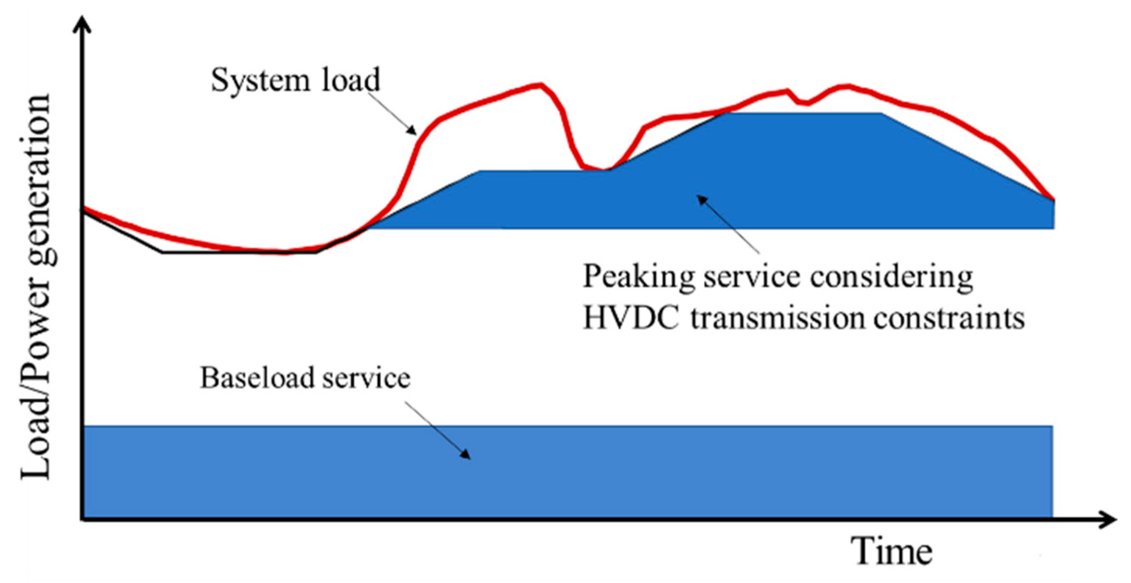
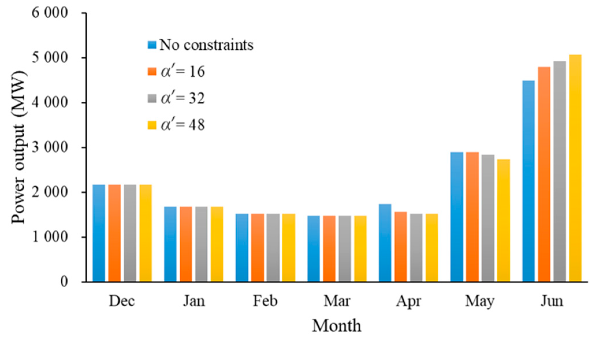
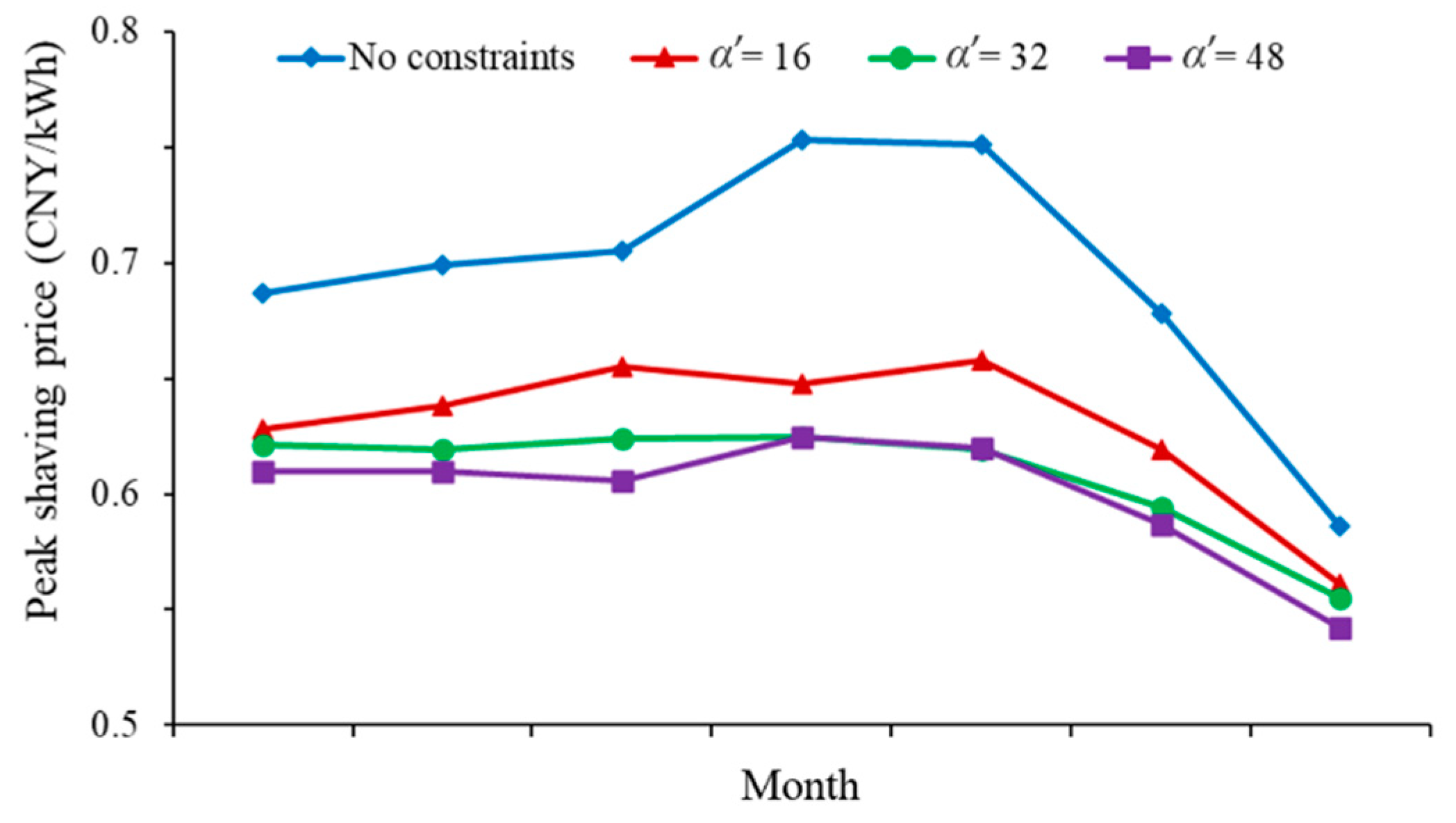
4.2. Effect of HVDC Transmission Stability Constraints

As described in Section 4.1, HVDC transmission stability constraints have a significant impact on energy prices. We investigated the effect of different α′ values on long-term power generation operation using the stochastic optimization model introduced in Section 2.3. Table 2 lists the main statistical results obtained from evaluating the long-term effects of different HVDC transmission constraints. The operating results varied significantly under different HVDC transmission constraints. In general, the stability constraints of HVDC transmission significantly limited the peak shaving ability of a hydropower plant. The increase in α′ caused an increase in the amount of power generation in response to the peak load, resulting in the inability to pursue high prices. Though the amount of power generation increased, the negative impact of the price decline dominated the relationship, resulting in a decline in overall revenue.
The corresponding expected reservoir storage trajectories and power output results can be seen in Figure 7 and Figure 8, respectively. It is evident that the hydropower plant tended to maintain a high generation efficiency when the stability duration was relatively long, and when HVDC transmission could be flexibly adjusted, the sequences of power generation are redistributed and high revenue could be obtained. For example, compared with that in the case of α′ = 48, the expected power generation was reduced by approximately 1.35% without stability constraints. As a trade-off, the expected power generation revenue increased by nearly 4.97%. Figure 9 shows the statistical expected peak shaving prices for various values of α′, and the baseload prices were equal at 0.476 CNY/kWh. Notably, a small α′ value was found to correspond to a high peak shaving price. Normally, monthly marginal peak shaving revenue decreases with increasing power generation. However, when power generation is relatively small, power generation dominates the peak price. Therefore, hedging this relation led to a reduction in power generation only in later time periods to avoid price decreases due to a large amount of power generation, as shown in Figure 7. As α′ decreased, hedging occurred earlier because of the relatively high price, as shown in Figure 6.
According to the actual operation records, the minimum stable operation duration of the XZ-line was 4 h in approximately 80% of the cases. Therefore, in the case studies in the following two subsections, the value of α′ was set to 16.

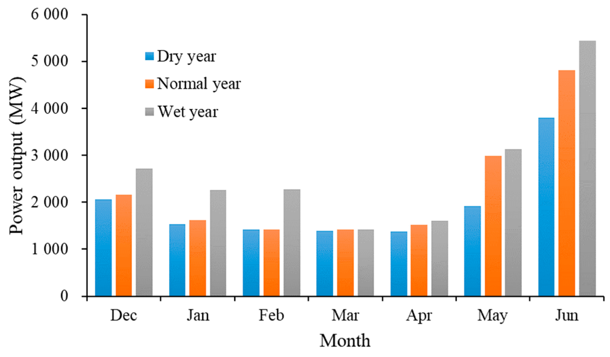
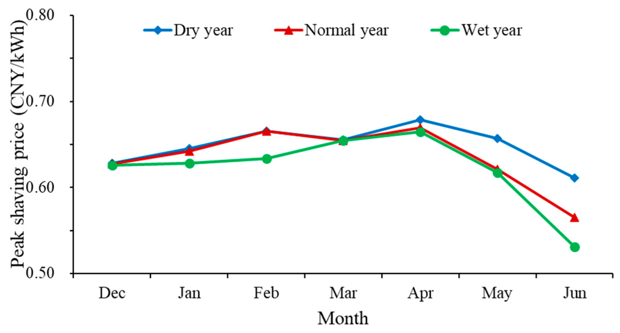
4.3. Operation Schemes in Different Inflow Scenarios

In this subsection, the sensitivity of the proposed model to varying reservoir inflows was investigated. Three representative inflow scenarios corresponding to dry, normal, and wet hydrological patterns were selected to simulate power generation operations. The corresponding reservoir storage trajectories and power output results are depicted in Figure 10 and Figure 11, respectively. The figure shows that under different inflow scenarios, the reservoir considered the ecological flow demand and generated electricity with natural inflow to maintain a high power generation efficiency until the preflood period. When the reservoir inflow gradually changed from a dry hydrological pattern to a wet pattern, there was a significant decline in the preflood water level because the reservoir inflow was relatively concentrated during preflood periods. To avoid a sharp decline in the peak shaving price, the surplus electricity was transferred to the previous periods. These findings imply that to maximize the cumulative revenue of short-term peak shaving operation, centralized power generation should be avoided in long-term operation, especially under wet hydrological patterns.
Figure 12 shows the statistical peak shaving prices under different inflow scenarios. As the reservoir inflow increased, the average peak shaving price decreased each month due to the increase in power generation. Table 3 lists the main statistical results for evaluating the long-term effects of different inflow scenarios, as well as the expected values of stochastic programming. In general, with the increase in reservoir inflow, the long-term power generation and revenue were found to increase significantly. Though the peak shaving price decreased with increasing reservoir inflow, the average electricity price showed an upward trend. In consideration of the minimum ecological flow demand, as the reservoir inflow increased, more electricity could be allocated during hours of high electricity prices, which means that peak shaving revenue could be increased. The above analysis indicates that under different inflow conditions, the hydropower operation model proposed in this paper can fully exploit the short-term peak shaving potential and ensure that the long-term cumulative revenue is maximized on the basis of satisfying the operating constraints.

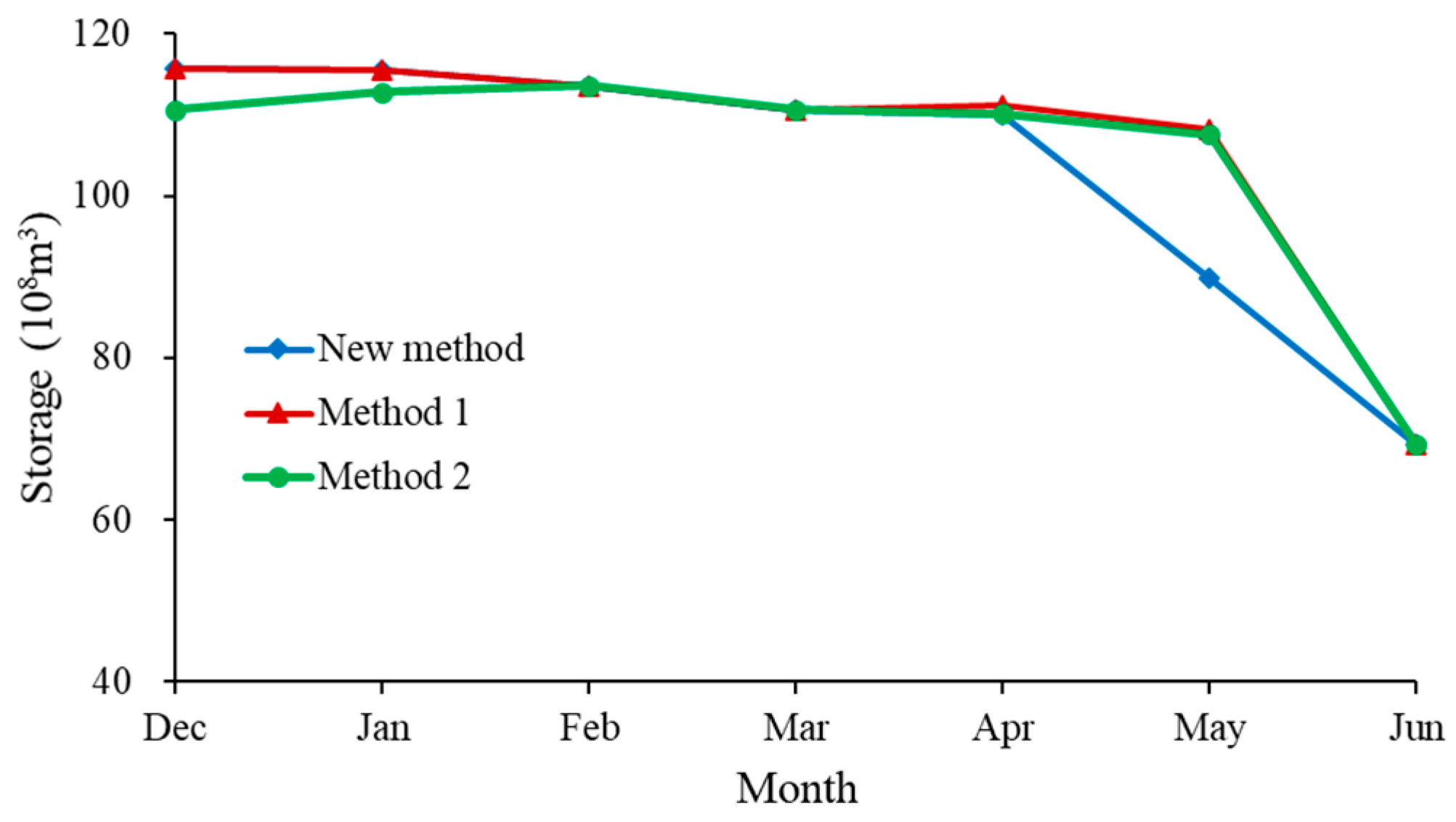
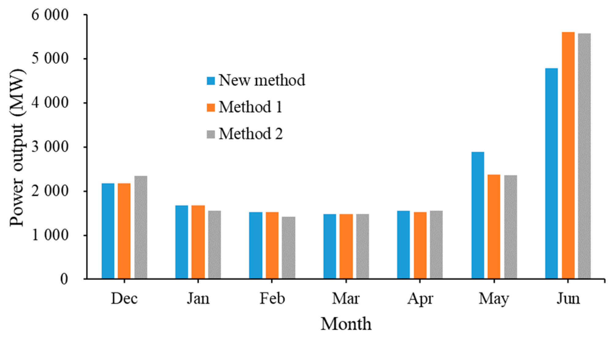
4.4. Performance Comparison

To examine the advantages and reliability of the proposed method, a comparison with two existing long-term hydropower optimization models was made by simulation. The two models corresponded to the traditional generation maximization model and the hydropower optimization model of Zambon et al. [43], respectively. The objective of the first model was to maximize the expected energy production for historical inflow scenarios. In this study, this model is referred to as Method 1, and it does not consider the demand of the receiving power grid. Zambon et al. [43] developed an integrated optimization model to optimize the Brazilian hydro–thermal system. The second model refers to the hydro part of the integrated model. This hydropower optimization model used a quadratic function as the objective to compensate for the deviation between energy production and load demand. This model is referred to as Method 2, and it can follow load demand variations while maximizing energy production. Both of the above models are subject to the operation constraints presented in Section 2.3. The monthly average load demand of the ZJPG was calculated from the historical data described in Section 3.2. In Method 2, the monthly load demand was assumed to be equal to the total demand minus the equivalent base load. As shown in Figure 13, the minimum load demand was set to the maximum transmission power of the XHP (6300 MW).
Table 4 lists the optimization results of Methods 1 and 2 under three typical inflow scenarios and the expected values for historical inflow scenarios. The results of the proposed method are shown in Table 3. It should be noted that the power generation revenues in Table 4 were calculated using the revenue estimation function (Equation (18)) in Section 2.3. It can be seen that, in terms of both energy production and revenue, the performance of Method 1 showed superiority to Method 2. Compared with Method 1, the expected energy production obtained by the newly proposed method was reduced by 1.57%. As a trade-off, the expected power generation revenue increased by 1.08%. Compared with Method 2, the expected power generation revenue of the proposed method increased by 1.48%, while the energy production loss was 1.1%. We moreover found that the improvement achieved by the proposed method was more obvious in years with high reservoir inflows. For example, compared with Method 2, the power generation revenues of the proposed method under the three typical inflow scenarios of dry, normal, and wet increased by 0.43%, 2.03%, and 3.22%, respectively. In summary, these results demonstrate that the method proposed in this paper can effectively improve long-term cumulative power generation revenue, although there was a small amount of power loss. The performance comparisons for historical inflow scenarios indicated the reliability of the proposed optimization model in ensuring the power generation revenue.
The expected reservoir storage trajectories and generation schedules from different solutions are depicted in Figure 14 and Figure 15, respectively. Methods 1 and 2 postponed storage depletion and maintained the highest hydraulic head to maximize power generation. However, due to the sufficient reservoir inflow, power generation was concentrated in later time periods, especially in June. In contrast, the new method generated more electricity before June than the other two methods, which alleviated the concentration of electricity and improved peak shaving performance. This improvement was mainly attributable to effective compromise by considering the demands of both the generation and receiving sides. Though Method 2 considers monthly load demand, it cannot guarantee the cumulative peak shaving revenue and may result in a loss of revenue due to reduced energy production. Considering the short-term peak shaving demands, the long-term operation scheme of the XHP can effectively distribute power generation in different time periods, thereby increasing revenue. Affected by ecological flow requirements and HVDC transmission constraints, the peak shaving capacity of the XHP greatly decreased, but the analysis of the above results demonstrated that the proposed method is useful for exploring the peak shaving potential.

5. Conclusions

In this study, we proposed an optimization model that incorporates peak shaving demands for the long-term operation of an IHP. To estimate the peak shaving revenue in long-term operation, a short-term simulation model with HVDC transmission constraints was established to obtain MA price curves that bridge two time-coupled operations. The MA price curves were incorporated into the long-term optimization model to maximize the expected power generation revenue in the considered inflow scenarios. To evaluate the proposed model, simulations with different conditions were conducted to evaluate the operation of the XHP in China during the drawdown season. The following conclusions were drawn from the analysis.
(1)
The MA price curves, which characterize the relationship between energy production and peak shaving revenue, verified that the marginal revenue of peak shaving decreases with increasing power generation.
(2)
HVDC transmission stability constraints significantly limit the peak shaving ability of the XHP, which leads to significant reductions in energy prices and generation revenue.
(3)
Compared with the existing optimization methods, the model proposed in this paper can effectively increase long-term cumulative power generation revenue, although we found a small reduction in energy production. Thus, the proposed approach is effective for exploring the revenue potential of interprovincial hydropower transmission to meet peak shaving demands.
In the future, more large hydropower plants will be put into operation in Southwest China, and more hydropower will be delivered to the load centers through HVDC transmission lines than currently delivered. It is important to fully exploit the flexibility of these hydropower plants to respond to the peak shaving requirements of the load centers. Therefore, research on the long-term operation of the XHP that considers the short-term peak shaving demands has significant reference value for the optimal operation of hydropower plants connected to HVDC transmission lines. The practical application of the proposed methodology can be extended to multiple receiving power grids with different electricity market environments. It is also recommended that further research be extended to large-scale hydropower transmission systems in other hydropower-rich countries, such as Brazil.

Author Contributions

Conceptualization, R.C. and J.S.; methodology, R.C.; software, J.W.; validation, J.S. and C.C.; formal analysis, R.C. and J.S.; investigation, R.C. and J.W.; writing—original draft preparation, R.C.; writing—review and editing, J.S. and C.C. All authors have read and agreed to the published version of the manuscript.

Funding

This work was supported by the Fundamental Research Funds for the Central Universities (grant number DUT19TD32, DUT19JC43).

Acknowledgments

The writers are very grateful to the anonymous reviewers and editors for their constructive comments.

Conflicts of Interest

The authors declare no conflict of interest.

References

  1. International Hydropower Association (IHA). 2019 Hydropower Status Report; IHA: London, UK, 2019. [Google Scholar]
  2. Li, Y.; Li, Y.B.; Ji, P.F.; Yang, J. The status quo analysis and policy suggestions on promoting China׳s hydropower development. Renew. Sustain. Energy Rev. 2015, 51, 1071–1079. [Google Scholar] [CrossRef]
  3. Zeng, M.; Peng, L.L.; Fan, Q.N.; Zhang, Y.J. Trans-regional electricity transmission in China: Status, issues and strategies. Renew. Sustain. Energy Rev. 2016, 66, 572–583. [Google Scholar]
  4. Shen, J.J.; Zhang, X.F.; Wang, J.; Cao, R.; Wang, S.; Zhang, J. Optimal Operation of Interprovincial Hydropower System Including Xiluodu and Local Plants in Multiple Recipient Regions. Energies 2019, 12, 144. [Google Scholar] [CrossRef] [Green Version]
  5. Farahmand, H.; Jaehnert, S.; Aigner, T.; Huertas-Hernando, D. Nordic hydropower flexibility and transmission expansion to support integration of North European wind power. Wind Energy 2015, 18, 1075–1103. [Google Scholar] [CrossRef]
  6. Hennig, T.; Wang, W.L.; Magee, D.; He, D.M. Yunnan’s Fast-Paced Large Hydropower Development: A Powershed-Based Approach to Critically Assessing Generation and Consumption Paradigms. Water 2016, 8, 476. [Google Scholar] [CrossRef]
  7. Xie, K.G.; Dong, J.Z.; Tai, H.M.; Hu, B.; He, H.L. Optimal planning of HVDC-based bundled wind-thermal generation and transmission system. Energy Convers. Manag. 2016, 115, 71–79. [Google Scholar] [CrossRef]
  8. Cheng, C.T.; Yan, L.Z.; Mirchi, A.; Madani, K. China’s booming hydropower: System modeling challenges and opportunities. J. Water Resour. Plan. Manag. 2017, 143, 1–5. [Google Scholar] [CrossRef]
  9. Ding, N.; Duan, J.H.; Xue, S.; Zeng, M.; Shen, J.F. Overall review of peaking power in China: Status quo, barriers and solutions. Renew. Sustain. Energy Rev. 2015, 42, 503–516. [Google Scholar] [CrossRef]
  10. Gu, Y.J.; Xu, J.; Chen, D.C.; Wang, Z.; Li, Q.Q. Overall review of peak shaving for coal-fired power units in China. Renew. Sustain. Energy Rev. 2016, 54, 723–731. [Google Scholar] [CrossRef]
  11. Ye, Y.J.; Huang, W.B.; Ma, G.W.; Wang, J.L.; Liu, Y.; Hu, Y.L. Cause analysis and policy options for the surplus hydropower in southwest China based on quantification. J. Renew. Sustain. Energy 2018, 10, 015908. [Google Scholar] [CrossRef]
  12. Su, C.G.; Cheng, C.T.; Wang, P.L.; Shen, J.J. Optimization Model for the Short-Term Operation of Hydropower Plants Transmitting Power to Multiple Power Grids via HVDC Transmission Lines. IEEE Access 2019, 7, 139236–139248. [Google Scholar] [CrossRef]
  13. Shen, J.J.; Cheng, C.T.; Wang, S.; Yuan, X.Y.; Sun, L.F.; Zhang, J. Multiobjective optimal operations for an interprovincial hydropower system considering peak-shaving demands. Renew. Sustain. Energy Rev. 2020, 120, 109617. [Google Scholar] [CrossRef]
  14. Hammons, T.J.; Lescale, V.F.; Uecker, K.; Haeusler, M.; Retzmann, D.; Staschus, K.; Lepy, S. State of the art in ultrahigh-voltage transmission. Proc. IEEE 2012, 100, 360–390. [Google Scholar] [CrossRef]
  15. Xie, M.F.; Zhou, J.Z.; Li, C.L.; Lu, P. Daily generation scheduling of cascade hydro plants considering peak shaving constraints. J. Water Resour. Plan. Manag. 2015, 142, 04015072. [Google Scholar] [CrossRef]
  16. Feng, Z.K.; Niu, W.J.; Cheng, C.T.; Zhou, J.Z. Peak shaving operation of hydro-thermal-nuclear plants serving multiple power grids by linear programming. Energy 2017, 135, 210–219. [Google Scholar] [CrossRef]
  17. Shen, J.J.; Cheng, C.T.; Cheng, X.; Lund, J.R. Coordinated operations of large-scale UHVDC hydropower and conventional hydro energies about regional power grid. Energy 2016, 95, 433–446. [Google Scholar] [CrossRef]
  18. Sreekanth, J.; Datta, B.; Mohapatra, P.K. Optimal short-term reservoir operation with integrated long-term goals. Water Resour. Manag. 2012, 26, 2833–2850. [Google Scholar] [CrossRef]
  19. Xu, B.; Zhong, P.A.; Stanko, Z.; Zhao, Y.F.; Yeh, W.W. A multiobjective short-term optimal operation model for a cascade system of reservoirs considering the impact on long-term energy production. Water Resour. Res. 2015, 51, 3353–3369. [Google Scholar] [CrossRef]
  20. Ming, B.; Liu, P.; Guo, S.L.; Cheng, L.; Zhang, J.W. Hydropower reservoir reoperation to adapt to large-scale photovoltaic power generation. Energy 2019, 179, 268–279. [Google Scholar] [CrossRef]
  21. English, J.; Niet, T.; Lyseng, B.; Keller, V.; Palmer-Wilson, K.; Robertson, B.; Wild, P.; Rowe, A. Flexibility requirements and electricity system planning: Assessing inter-regional coordination with large penetrations of variable renewable supplies. Renew. Energy 2020, 145, 2770–2782. [Google Scholar] [CrossRef]
  22. Morillo, J.L.; Zephyr, L.; Perez, J.F.; Anderson, C.L.; Cadena, A. Risk-averse stochastic dual dynamic programming approach for the operation of a hydro-dominated power system in the presence of wind uncertainty. Int. J. Electr. Power Energy Syst. 2020, 115, 105469. [Google Scholar] [CrossRef]
  23. Madani, K.; Lund, J.R. Modeling California′s high-elevation hydropower systems in energy units. Water Resour. Res. 2009, 45. [Google Scholar] [CrossRef]
  24. Olivares, M.A.; Lund, J.R. Representing energy price variability in long-and medium-term hydropower optimization. J. Water Resour. Plan. Manag. 2012, 138, 606–613. [Google Scholar] [CrossRef]
  25. Ak, M.; Kentel, E.; Savasaneril, S. Operating policies for energy generation and revenue management in single-reservoir hydropower systems. Renew. Sustain. Energy Rev. 2017, 78, 1253–1261. [Google Scholar] [CrossRef]
  26. Moreira, A.; Pozo, D.; Street, A.; Sauma, E. Reliable renewable generation and transmission expansion planning: Co-optimizing system′s resources for meeting renewable targets. IEEE Trans. Power Syst. 2016, 32, 3246–3257. [Google Scholar] [CrossRef]
  27. Zhang, H.X.; Lu, Z.X.; Hu, W.; Wang, Y.T.; Dong, L.; Zhang, J.T. Coordinated optimal operation of hydro-wind-solar integrated systems. Appl. Energy 2019, 242, 883–896. [Google Scholar] [CrossRef]
  28. Zhao, L.; Yang, Z.Y.; Lee, W.J. The impact of time-of-use (TOU) rate structure on consumption patterns of the residential customers. IEEE Trans. Ind. Appl. 2017, 53, 5130–5138. [Google Scholar] [CrossRef]
  29. Yang, H.J.; Wang, L.; Zhang, Y.Y.; Ma, Y.H.; Zhou, M. Reliability evaluation of power system considering time of use electricity pricing. IEEE Trans. Power Syst. 2018, 34, 1991–2002. [Google Scholar] [CrossRef]
  30. Wu, X.Y.; Li, S.M.; Cheng, C.T.; Miao, S.M.; Ying, Q.L. Simulation-Optimization Model to Derive Operation Rules of Multiple Cascaded Reservoirs for Nash Equilibrium. J. Water Resour. Plan. Manag. 2019, 145, 04019013. [Google Scholar] [CrossRef]
  31. Castro, P.M.; Grossmann, I.E. Generalized disjunctive programming as a systematic modeling framework to derive scheduling formulations. Ind. Eng. Chem. Res. 2012, 51, 5781–5792. [Google Scholar] [CrossRef]
  32. Tong, B.; Zhai, Q.Z.; Guan, X.H. An MILP Based Formulation for Short-Term Hydro Generation Scheduling with Analysis of the Linearization Effects on Solution Feasibility. IEEE Trans. Power Syst. 2013, 28, 3588–3599. [Google Scholar] [CrossRef]
  33. Feng, Z.K.; Niu, W.J.; Wang, W.C.; Zhou, J.Z.; Cheng, C.T. A mixed integer linear programming model for unit commitment of thermal plants with peak shaving operation aspect in regional power grid lack of flexible hydropower energy. Energy 2019, 175, 618–629. [Google Scholar] [CrossRef]
  34. Xu, B.; Boyce, S.E.; Zhang, Y.; Liu, Q.; Guo, L.; Zhong, P.A. Stochastic Programming with a Joint Chance Constraint Model for Reservoir Refill Operation Considering Flood Risk. J. Water Resour. Plan. Manag. 2017, 143, 04016067. [Google Scholar] [CrossRef]
  35. Li, X.; Li, T.J.; Wei, J.H.; Wang, G.Q.; Yeh, W.W.G. Hydro unit commitment via mixed integer linear programming: A case study of the Three Gorges Project, China. IEEE Trans. Power Syst. 2014, 29, 1232–1241. [Google Scholar] [CrossRef]
  36. Gau, C.Y.; Schrage, L.E. Implementation and testing of a branch-and-bound based method for deterministic global optimization: Operations research applications. In Frontiers in Global Optimization; Floudas, C.A., Pardalos, P.M., Eds.; Springer: Boston, MA, USA, 2004; Volume 74, pp. 145–164. [Google Scholar]
  37. Zhu, F.L.; Zhong, P.A.; Sun, Y.M.; Yeh, W.W.G. Real-time optimal flood control decision making and risk propagation under multiple uncertainties. Water Resour. Res. 2017, 53, 10635–10654. [Google Scholar] [CrossRef] [Green Version]
  38. Xu, B.; Zhu, F.L.; Zhong, P.A.; Chen, J.; Liu, W.F.; Ma, Y.F.; Guo, L.; Deng, X.L. Identifying long-term effects of using hydropower to complement wind power uncertainty through stochastic programming. Appl. Energy 2019, 253, 113535. [Google Scholar] [CrossRef]
  39. Wang, J.; Cheng, C.T.; Wu, X.Y.; Shen, J.J.; Cao, R. Optimal Hedging for Hydropower Operation and End-of-Year Carryover Storage Values. J. Water Resour. Plan. Manag. 2019, 145, 04019003. [Google Scholar] [CrossRef]
  40. Zhou, Y.L.; Guo, S.L.; Liu, P.; Xu, C.Y. Joint operation and dynamic control of flood limiting water levels for mixed cascade reservoir systems. J. Hydrol. 2014, 519, 248–257. [Google Scholar] [CrossRef]
  41. Mu, J.; Ma, C.; Zhao, J.Q.; Lian, J.J. Optimal operation rules of Three-gorge and Gezhouba cascade hydropower stations in flood season. Energy Conv. Manag. 2015, 96, 159–174. [Google Scholar] [CrossRef]
  42. Tilmant, A.; Kelman, R. A stochastic approach to analyze trade-offs and risks associated with large-scale water resources systems. Water Resour. Res. 2007, 43. [Google Scholar] [CrossRef]
  43. Zambon, R.C.; Barros, M.T.L.; Lopes, J.E.G.; Barbosa, P.S.F.; Francato, A.L.; Yeh, W.W.G. Optimization of large-scale hydrothermal system operation. J. Water Resour. Plan. Manag. 2012, 138, 135–143. [Google Scholar] [CrossRef]
Figure 1. Methodological framework of the proposed optimization model. MILP: mixed-integer linear programming; MA: moving average; and NLP: nonlinear programming.
Energies 13 04804 g001
Figure 2. Power generation considering high-voltage direct current (HVDC) transmission constraints.
Energies 13 04804 g002
Figure 3. Schematic diagram of the MA price curve for a typical daily load scenario.
Energies 13 04804 g003
Figure 4. Monthly inflow data for the long-term operation model.
Energies 13 04804 g004
Figure 5. Typical scenarios for (a) daily load and (b) MA price curves.
Energies 13 04804 g005
Figure 6. MA price curves with different HVDC transmission stability constraints. α′: set of time periods for stable power output.
Energies 13 04804 g006
Figure 7. Expected reservoir storage trajectories under different HVDC transmission constraints.
Energies 13 04804 g007
Figure 8. Power output results under different HVDC transmission constraints.
Energies 13 04804 g008
Figure 9. Statistical peak shaving prices under different HVDC transmission constraints.
Energies 13 04804 g009
Figure 10. Reservoir storage trajectories under different inflow scenarios.
Energies 13 04804 g010
Figure 11. Power output results under different inflow scenarios.
Energies 13 04804 g011
Figure 12. Statistical peak shaving prices under different inflow scenarios.
Energies 13 04804 g012
Figure 13. The monthly load demand corresponding to Method 2.
Energies 13 04804 g013
Figure 14. Expected reservoir storage trajectories of different optimization models.
Energies 13 04804 g014
Figure 15. Expected monthly generation schedules of different optimization models.
Energies 13 04804 g015
Table 1. Parameters for the Xiluodu hydropower plant (XHP) and the Xiluodu–Zhejiang HVDC transmission line (XZ-line).
ComponentParameterValueUnit
Reservoir of XHPInstalled capacity12,600MW
Normal water level600.00m
Dead water level540.00m
Flood-limited water level560.00m
Active storage64.6108 m3
Minimum ecological flow1400m3/s
XZ-lineTransmission capacity8000MW
Maximum ramping capacity (ΔPH)600MW
Table 2. Operational performance evaluation under different HVDC transmission constraints.
Factor Case ( α ) Power Generation (108 kWh)Total Revenue (108 CNY)Average Price (CNY/kWh)Peak Price (CNY/kWh)Baseload Price (CNY/kWh)
No constraints114.9563.520.5530.6470.476
16115.961.510.5310.5970.476
32116.2060.910.5240.5820.476
48116.5260.510.5190.5710.476
Table 3. Operational performance evaluation under different inflow scenarios.
Hydrological PatternPower Generation (108 kWh)Total Revenue (108 CNY)Average Price (CNY/kWh)Peak Price (CNY/kWh)
Dry97.1851.370.5290.627
Normal114.7960.950.5310.599
Wet135.6872.660.5360.588
Expected value115.961.510.5310.597
Table 4. Comparison results of Methods 1 and 2.
Hydrological PatternModelsPower Generation (108 kWh)Total Revenue (108 CNY)Average Price (CNY/kWh)
DryMethod 197.7251.260.525
Method 297.5751.150.524
NormalMethod 1117.0159.920.512
Method 2116.7459.740.512
WetMethod 1138.6171.940.519
Method 2136.0570.390.517
Expected valueMethod 1117.7560.850.517
Method 2117.1960.610.517

