Abstract
Soot formation in combustion systems is a growing concern due to its adverse environmental and health effects. It is considered to be a tremendously complicated phenomenon which includes multiphase flow, thermodynamics, heat transfer, chemical kinetics, and particle dynamics. Although various numerical approaches have been developed for the detailed modeling of soot evolution, most industrial device simulations neglect or rudimentarily approximate soot formation due to its high computational cost. Developing accurate, easy to use, and computationally inexpensive numerical techniques to predict or estimate soot concentrations is a major objective of the combustion industry. In the present study, a supervised Artificial Neural Network (ANN) technique is applied to predict the soot concentration fields in ethylene/air laminar diffusion flames accurately with a low computational cost. To gather validated data, eight different flames with various equivalence ratios, inlet velocities, and burner geometries are modeled using the CoFlame code (a computational fluid dynamics (CFD) parallel combustion and soot model) and the Lagrangian histories of soot-containing fluid parcels are computed and stored. Then, an ANN model is developed and optimized using the Levenberg-Marquardt approach. Two different scenarios are introduced to validate the network performance; testing the prediction capabilities of the network for the same eight flames that are used to train the network, and for two new flames that are not within the training data set. It is shown that for both of these cases the ANN is able to predict the overall soot concentration field very well with a relatively low integrated error.
1. Introduction
Soot emissions from combustion processes have damaging effects on both the environment and human health. Soot is the general term used for the class of pollutants known as PM 2.5, which constitutes particulate matter with a diameter less than or equal to 2.5 micrometers [1,2]. The minute nature of the soot particle makes it especially harmful when inhaled by an individual as it quite easily reaches the lungs and bloodstream. It can then lead to a host of serious issues including heart attacks, bronchitis, asthma, strokes, and even death [3]. Furthermore, soot is a notable contributor to climate change, second only to CO2 [4]. Larger soot aggregates and the smaller soot particulate matter both contribute to the problem. The smaller, lighter particulates remain in the air absorbing sunlight and subsequently warming the surrounding air. On the other hand, the larger, heavier aggregates fall to the ground and absorb sunlight there. As a result, any surrounding snow or ice is melted far faster [4].
The problems outlined above are concerning, thus stricter regulations on soot emissions are becoming commonplace. This is true especially in current times, when efforts to be environmentally sustainable are at an all-time high and are at the forefront of much in-depth research. For example, new vehicles sold in the European Union and European Economic Area (EEA) member states have rigorous regulations placed upon them [5]. Unfortunately for engine designers worldwide, soot formation is an exceptionally complex phenomenon dependent on numerous physical and chemical processes such as reaction kinetics, thermodynamics, heat transfer, and particle dynamics. The implementation of Computational Fluid Dynamics (CFD) throughout the engine design process has now become mainstream. However, if soot formation mechanisms were considered as part of these simulations, the computational costs would quickly become intractable if any respectable accuracy is to be obtained [6]. Currently, prototypes must be manufactured in order to be certain of the soot emissions a given engine will produce. This time-consuming, expensive, and strenuous method has limited the improvement in this area as many manufacturers are not willing to put forth this great effort to discover the soot emissions of a given engine. The balance between computational cost and accuracy of results quickly presents itself as an obstacle for this industry, as it often does for many others.
In CFD simulations, numerical accurate modelling and prediction of soot properties, such as concentration and particle size and shape, remains challenging due to the collective chemical, physical and thermodynamic interactions, and multiphase flow [7,8]. Previous numerical studies of soot evolution in laminar and turbulent flames have been based on different levels of fidelity. Many of these previous studies have utilized semi-empirical soot models coupled with simplified combustion models. In these studies, soot concentrations have generally not been predicted with acceptable accuracy, with errors in soot concentration ranging from one to two orders of magnitude or more [7,9,10,11]. Conversely, some studies use more accurate soot models, like the soot model explained in the CoFlame code [12] and hybrid method of moments (HMOM) developed by Mueller et al. [13], that allow for the description of soot volume fraction, number density, and morphology of the aggregates. In these models, in addition to the influence of local concentrations of various species, temperature, and pressure, the effects of various chemical and physical phenomena such as particle nucleation from Polycyclic Aromatic Hydrocarbons (PAHs), PAH dimer condensation, physical coagulation, surface growth by the hydrogen-abstraction˗carbon-addition (HACA) mechanism, oxidation, and oxidation-induced fragmentation on soot evolution are considered [12,14,15]. Simulating all the aromatic precursors and the phenomena mentioned above causes the high-fidelity soot models to be computationally expensive.
To model soot evolution in turbulent flames, several Large Eddy Simulation (LES) studies have been attempted [7,8,11]. In general, in addition to modelling soot and precursor chemistry, the high fidelity LES-based models comprise models for turbulence-soot-chemistry interactions at the subfilter scale [8]. In this case, uncertainties related to the models of subfilter fluctuations would be added to the uncertainties associated with the soot model and the chemical kinetic mechanism [8,16]. It should be pointed out that the models of subfilter fluctuations depend on the employed soot model (for instance, state-of-the-art models of subfilter fluctuations are based on HMOM soot model [8,13]). Therefore, by changing the soot model, the models of subfilter fluctuations need to be modified [7]. Furthermore, one of the most important issues relates to the errors associated with combustion models [8,16], which can affect the soot prediction significantly. As an example, the recent work of Wick et al. [16] is worth mentioning here. They performed an investigation to show how errors related to combustion models (for example, flamelet models) propagate through into the mechanisms of soot characteristic prediction via interactions between the gas and solid phase. In their work, the coupling of a Flamelet/Progress Variable model with the HMOM soot model was analysed using Direct Numerical Simulation (DNS) results [15], where the same soot model (HMOM) was used. It was found that there are significant errors in the predicted soot field, which are traced back to tabulated quantities in the flamelet library propagating through the computation via PAH-based growth rates. Overall, this body of work indicates that LES-based soot models are still limited and more studies should be conducted to improve these models. However, it is clear that to model soot evolution, not only is a combustion model needed, along with a soot model and models for subfilter scale turbulence-soot-chemistry interactions, but all the aromatic precursors as well as the physics involved (for instance, aromatic collision or PAH condensation) should be simulated, which is a challenging task and computationally expensive. Conversely, as mentioned above, the low-cost and precise estimation of soot properties, such as concentration, has become highly desired for industry. Therefore, to tackle this controversy, a novel soot estimator concept has been recently developed and validated [6,17,18,19].
The idea of linking a post-processing tool to CFD simulations to estimate soot characteristics accurately with a low computational cost was first proposed by Bozorgzadeh [19]. As a proof of concept, a post-processing technique for laminar flames was proposed by Alexander et al. [6] in 2018. The aforementioned work has been further amended where accuracy was improved and turbulent flame data was used, albeit with limited success [18,19]. The prediction method described in these papers is a rudimentary library consisting of a collection of data arrays from which desired values can be interpolated. The most recent work [18] demonstrates exceptional success when estimating the soot volume fraction of nine different steady laminar flames when the library comprises data of the same nine flames being tested.
Theoretically, the rate of soot formation (or destruction) can be thought to depend entirely on local system characteristics at any point in time t as
where , , , and are the temperature, the mass fraction of species i, the pressure, the soot volume fraction (concentration), and the average soot surface area, respectively. The idea of a soot estimator was based on this assumption that to calculate , libraries (like the thermodynamic tables) can be created in which the values of different variables such as temperature and mass fractions are stored. However, due to the longer timescales of soot formation as compared to those of flow and gas-phase chemistry, and the inherent non-linearity of the problem, soot characteristics cannot be considered to be related only to especially local properties [18]. Veshkini et al. [20] and Kholghy et al. [21] showed that soot evolution is a stronger function of the temporal history of soot particles than just local flame characteristics. Therefore, within the soot estimator approach [6,17,18], it was assumed that the local instantaneous soot volume fraction is a function of the temporal history of key variables in a combustion process. The fundamental formula from which the soot estimator concept was developed is as follows:
where , , , and are the temperature time-integrated history, the mass fraction history of species i, the pressure history, the time-integrated history of soot volume fraction, and the average soot surface area history, respectively.
By using the soot estimator approach, Alexander et al. [6] and Zimmer et al. [18] showed that it is possible to estimate soot volume fraction, in an uncoupled manner, by tracking the histories of certain properties (temperature, species concentration) of fluid parcels. Therefore, only the gas phase conservation equations for mass, momentum, energy, and species mass fraction need to be solved in a simulation, and different soot-related terms such as soot nucleation, coagulation, etc., which are typically included in advanced soot models as well as the statistical particle dynamics equations (for example, see the equations of conservation of soot aggregate number density and conservation of soot primary particle number density in the CoFlame code [12]) are not required to be solved. Therefore, much less computational effort would be needed.
For applying the soot estimator approach, at first, the gas-phase temperature, pressure, species mass fractions, etc. (the parameters on the right side of Equation (2)) should be obtained from a validated sooting flame model. Alexander et al. [6] and Zimmer et al. [18] used the CoFlame code to gather these parameters for nine different flames. Then, in these studies, the Lagrangian temporal histories of soot-containing fluid parcels were stored. They defined a specific number of dimensions to the library, corresponding to the variable histories that were being considered, and a specific number of bins in each dimension. The soot volume fraction resulting from each fluid parcel history, corresponding to those variable histories, were then stored in each bin. Due to practical constraints encountered in those works, only a few parameters could be stored in the library. In Reference [18], three data dimensions (the histories of temperature, mixture fraction, and hydrogen radical concentration) were used to estimate :
where is the mixture fraction history. In their work [18], 300 bins of refinement in each dimension was also assumed so that a 300 × 300 × 300 bin library, from which to interpolate, was created. Using this approach, the computational cost was kept moderate due to the reasons stated above. Furthermore, compared to the detailed numerical simulations (obtained from the CoFlame code where the gas-phase, as well as soot partial differential equations, were solved numerically), the average integrated error for prediction of the entire soot field across all flames was 0.42% [18]. However, the drawback of the method became evident when extending to transient and turbulent flows, where the timescales of the data are much larger, and the limited refinement of the data array becomes evident [17].
From the above discussion, it becomes clear that the accuracy of the approach developed previously [6,17,18] depends on the number of data dimensions and the number of bins. The work presented in Reference [18] was limited to three data dimensions and 300 bins of refinement in each dimension to avoid memory and compute time issues associated with dimensionality. The memory requirement in this approach [6,17,18] is a serious hindrance. Considering the example of a 300 × 300 × 300 library, the method implemented in the previous work requires multiple arrays that have lengths equal to the total number of bins, that is 300 × 300 × 300 = 27,000,000. Creating a 1 × 27,000,000 array using MATLAB R2018a requires 0.216 GB. This allows many arrays of the same size to be created with no issues. However, scaling to an additional dimension in search of further algorithm capability, the mesh now becomes a 300 × 300 × 300 × 300 field with a total of 8,100,000,000 bins. Creating a similar array to the one mentioned earlier with the updated number of bins will cost 60.3 GB, and therefore multiple arrays of this size cannot be created on a personal computer. A compromise in the number of dimensions used, or the number of bins per dimension, must then be made, hindering the scientific assessment of accuracy.
If the latter approach is chosen and the number of dimensions is increased to four while the number of bins is decreased to compensate, the idea of sparsity becomes more evident. When increasing the dimensions of the data field being analyzed, the available data quickly fills a smaller and smaller area of the entire field. With respect to the bin approach used in previous works, this would mean that the data would only fill a tiny portion of the millions of available bins. This is an inefficient use of memory and computational power. However, if added dimensions are not considered, plenty of available data is essentially discarded as it is not considered at all. These reasons, amongst others, inspired the notion of discovering a new method with which the post-processing tool can be implemented.
In the current work, a Neural Network is generated and taught by data from the CoFlame code [12] as a post-processing tool to estimate the soot volume fraction numerically with a low computational cost at various conditions. As mentioned above, this tool is necessary because, in industrial device simulations, soot formation is typically neglected or rudimentarily approximated due to high computational cost. The tool developed in this study would be able to estimate soot characteristics while it only needs properties from the gas-phase conservation equations (mass, momentum, energy and species mass fractions) as inputs. Therefore, the cost-benefit would be considerable since the soot-related terms and equations are not required to be solved in the flow model (the soot quantities such as volume fraction are obtained from the trained network using the model data as inputs). In the present study, issues of dimensionality that were observed previously in the library-based soot estimator models are less prevalent. This advantage will be crucial toward extending the concept of the soot estimator to transient and turbulent flames. However, it is worth mentioning that any error in the CFD model results can propagate into the estimator framework because the input/output datasets are directly obtained from the CFD simulations. As CFD simulations get more accurate, and more and more data are used to teach the network, this error propagation effect will diminish. It should be noted that, to the authors’ best knowledge, the present work is the first attempt to train artificial neural networks (ANNs) based on detailed modeling of soot formation. The methodology, fundamentals of ANN, data pre-processing, and network training are discussed in the following section. In the results section, the ANN predictions as well as its performance and error analysis are explained.
2. Methodology
Although not an entirely new concept, ANNs have recently become more prevalent due to their amazing flexibility and plethora of use cases. Before investigating the advantages of this method and precisely why it was preferred to others, it is important to establish an introductory level of knowledge about the actual processes going on within the model. A basic representation of the architecture of an ANN can be seen in Figure 1 below.
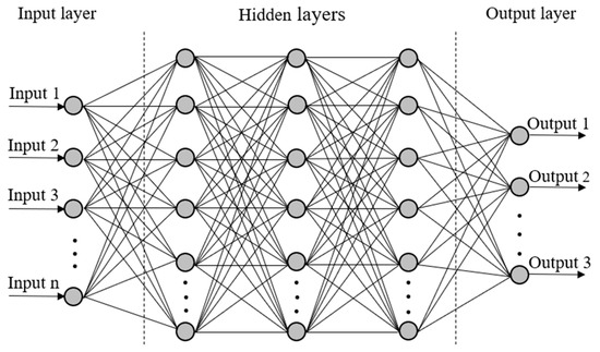
Figure 1.
A schematic representation of an artificial neural network.
Inspecting this architecture, it is clear to see that there are three main sections to examine. Each section can be referred to as a layer; at a minimum, every ANN will have at least three layers, the input, output, and hidden layers. While every single network is limited to only one input and one output layer, the number of hidden layers between them can be arbitrarily set to any number, wholly dependent on the desired accuracy and available computational power [22]. In general, the simplest ANN has only one hidden layer, while deep neural networks have multiple hidden layers. Similarly, each layer consists of a number of hidden nodes, or neurons, where calculations take place. The input and output layers are limited in the number of neurons they can have by the number of input variables being provided and the number of output variables desired by the user. Once again, the hidden layers are the flexible part of the network. As such, the number of neurons in the hidden layers remains unlimited in theory [22]. The basic premise of the network is that any neuron in a given layer is connected to every single neuron in the layers immediately surrounding it. Each connection between two neurons has a weight associated with it. The output from a given neuron is obtained by applying a non-linear function to the weighted sum of inputs to that neuron and an overall bias. The weights and biases are initially random; however, they are adjusted as the network learns from the data provided to it. The non-linear function within each neuron that is central to the calculations is referred to as the activation function [22]. Many functions are available for use; however, two commonly used ones are the hyperbolic tangent and the rectified linear unit (ReLU) functions [23]. Figure 2 shows a schematic representation of an individual neuron unit, including the various inputs and outputs. The figure depicts inputs x1, x2, … xj, each with a corresponding weight w1, w2, … wj, the summation function with bias, b, and the activation function f, which leads to the output. In addition, the hyperbolic tangent as well as ReLU activation functions are shown in Figure 3. As can be seen, tanh can only vary between −1 and 1. Moreover, tanh, as well as it’s derivative, are both monotonic functions. Put more explicitly, the output of a neuron with the hyperbolic tangent activation function is
and for the ReLU activation function, it is
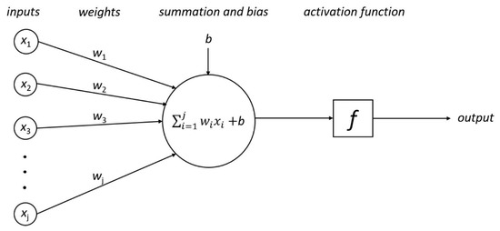
Figure 2.
A schematic representation of a single neuron.
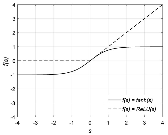
Figure 3.
The hyperbolic tangent and the rectified linear unit (ReLU) functions.
In the present study, the concept of supervised learning is utilized. Supervised learning is a type of machine learning model in which the relationship between the input and output of a system is obtained based on a given training sample of input-output pairs. The objective of supervised learning is to teach an artificial system like the neural network a way to map inputs to outputs, using the prescribed structure, so that the output can quickly be determined for any set of inputs fed [24]. For supervised learning, the entire data set is often split into three subsections; the training, validation, and testing sets. The training set is usually the largest and it comprises the data that is fed into the network as a way for it to learn from the data and adjust itself based on the error. The validation set is used to measure the generalization of the network—essentially how well the network will perform with unseen data. This subset is particularly important because it will serve to provide an indicator as when to stop training. If the generalization of the network stops improving, the training will be discontinued as a means of preventing overfitting, which is when the neural network over-trains itself such that it is well-suited to the particular training data, but will not reproduce results well that are outside of this data set. The testing data set is very similar to the validation set, in that they both consist of unseen data not used for training, with the only difference being the fact that the testing set has no impact on the learning done by the network. Therefore, it simply exists as a way to provide an independent measure of success.
In the current study, a backpropagation algorithm is applied to train the network. The specific algorithm used is referred to as ‘Levenberg-Marquardt backpropagation’. The method is used to determine the optimal network weights and biases which minimize error. In general, in the backpropagation algorithms, for every input-output pair in the training set, the input is first received and processed by the network and an output is obtained. The output on the first iteration is calculated by using randomly assigned weights and biases. The calculated output is then compared to the actual desired output from the input-output pair and an error is found. This error is then propagated back through the layers of the network and the weights of each connection and the biases of each neuron are adjusted accordingly. The process is then simply repeated until a global minimum of the error is found. For example, in the Levenberg-Marquardt training algorithm, the weight and bias values are updated using the following formula [25,26]:
where stands for the weights or biases, is the vector of network errors, is called regularization parameter or combination coefficient and is a positive number adjusted by the algorithm, and is the Jacobian matrix comprising first derivatives of the network errors with respect to the weights and biases. The matrix is typically calculated using the backpropagation algorithm stated above [25,26]. It is worth mentioning that the Levenberg-Marquardt algorithm is the combination of the gradient descent and the Newton algorithms. When is very close to zero, the Levenberg-Marquardt algorithm converts to the Newton algorithm. Conversely, when is very large, it becomes the gradient descent method. It should be also noted that the mentioned algorithm does not always work properly, as the network may get stuck on a local minimum. More information about the Levenberg-Marquardt algorithm as well as proof of the above equation are available in Reference [26].
ANNs have been successfully used to represent the chemistry in the simulation of laminar and turbulent flames with satisfactory results, negligible memory demand, and low computational cost (see References [27,28,29,30,31,32,33,34,35,36,37]). In addition, it should be pointed out that in a few fundamental studies, ANNs were trained using experimental data and then applied to predict soot properties. For instance, Inal et al. [38] experimentally studied soot characteristics in laminar, premixed, hydrocarbon fuel/oxygen/argon flames, and utilized ANN models to forecast the soot concentrations and particle sizes. At first, the soot characteristics were measured using classical light scattering techniques. Then, by using the input/output data sets obtained from the experiments, two neural network models were developed. In that work, the authors explained that they were not able to train and test a network to predict the soot number density with sufficient accuracy, due to great uncertainty in the determination of this parameter and a large minimum-maximum range.
In another study, Inal [39] developed a network to estimate PAH concentrations in laminar, premixed n-heptane/oxygen/argon and n-heptane/oxygen/oxygenate/argon flames. For data acquisition, an experimental study was performed. It was shown that the PAH amount was a strong function of equivalence ratio, mole fractions of C4 species, and presence of fuel oxygenates. The present study advances upon these works with full ex-situ prediction of soot concentration using ANNs.
In the present work, the input/output datasets are obtained from the CoFlame code [12]. CoFlame has been used extensively by multiple research groups to study a wide variety of axisymmetric laminar diffusion flames including those at microgravity and high pressure [40,41,42]. It is worth mentioning that CoFlame solves for soot primary particle number density and soot aggregate number density equations in addition to the conservation equations for mass, momentum, energy, and species mass [12]. The CoFlame sectional particle dynamics model contains nucleation, PAH condensation, HACA surface growth, surface coagulation, oxidation, fragmentation, particle diffusion, and thermophoresis. Radiation is also modeled using the discrete-ordinates method [12]. The boundary conditions and the coordinates (r and z) utilized in the code as well as the structure of a laminar coflow diffusion flame are shown in Figure 4.
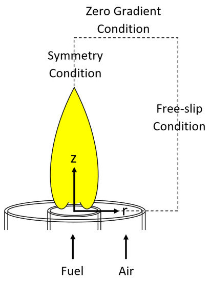
Figure 4.
A schematic representation of a laminar diffusion flame along with the coordinates (r, z) and the boundary conditions used in the CoFlame code (adapted from Reference [40]).
The results of the simulations of eight different ethylene–air laminar flames at atmospheric pressure are considered in the current study (see Table 1). These flames range from low to moderate soot volume fraction. The computed peak values, obtained from the CoFlame code (Veshkini et al. [20]), are reported in Table 1. For each flame, the values of eleven key variables including temperature (T), mixture fraction (MF), oxygen (O2), carbon monoxide (CO), carbon dioxide (CO2), hydrogen (H2), water (H2O), hydroxide (OH), acetylene (C2H2), benzene (A1), and soot volume fraction (fv) are gathered. As an example, the temperature contours for the flames SM32 and SM80 are shown in Figure 5. It should be pointed out that the first eight variables are considered key variables found in any combustion system. However, acetylene and benzene are included since they are the major species which result in PAH formation and hence affect soot inception and surface reactions. The soot volume fraction is the output in the present study.

Table 1.
The main characteristics of eight laminar flames (Experimental works of a Smooke et al. [43], and b Shaddix and Smyth [44] referred to as “SMXX” and “SYXX”, respectively).
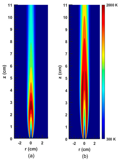
Figure 5.
2D contour plots of the temperature for the flames: (a) SM32; (b) SM80; obtained from the CoFlame code.
As previously mentioned, one of the problems associated with the binning process that was used in previous works is that it scales extremely poorly to added dimensions [6,17,18]. This also leads to large amounts of data being left unused (compare Equation (3) with Equation (2)). As a result, one of the first aspects that were explored with the ANN model was to increase the input parameters to exceed the three or four previously used.
In this study, similar to the work of Zimmer et al. [18], the Lagrangian histories of soot-containing fluid parcels are considered as the input datasets, and one network is trained for all the flames. In other words, the temperature history (Th), mixture fraction history (MFh), oxygen history (O2,h), carbon monoxide history (COh), carbon dioxide history (CO2,h), hydrogen history (H2,h), water history (H2Oh), hydroxide history (OHh), acetylene history (C2H2,h), and benzene history (A1h) are calculated and considered as the input dataset. To calculate the Lagrangian histories and create the library/data-frame the following steps are taken:
- (1)
- Gathering numerical data: as mentioned, the values of different parameters (such as temperature and oxygen) for the eight flames are gathered.
- (2)
- Extracting pathlines: each pathline was computed from the following ordinary differential equation:where is the current point in space of a fluid parcel which may contain soot, and which follows the fluid velocity with respect to time . In addition, is the initial position for each pathline and is the total number of pathlines.
- (3)
- Computing histories from pathlines: The history of a variable referred to the time integration of a given variable over its entire existence; for soot that is from inception to oxidation (that is along a pathline). For instance, for a general variable (Z), the history of Z is defined as:In previous studies [6,17,18], a specific number of bins was defined to divide the range of each history.
- (4)
- Storing soot concentrations: once the histories were computed for each fluid parcel pathline, the histories, as well as the associated soot concentration values, were stored in the libraries [6,17,18].
- (5)
- Concatenating the eight libraries/data-frames and generating one library/data-frame.
The key parts of the mentioned steps and the model flow are shown schematically in Figure 6. As can be seen, after training the network and finding the soot volume fraction along each fluid parcel pathline, linear interpolation is used to distribute the estimated fv on the r-z coordinate system (see Figure 6). It should be noted that in previous works [6,17,18], the aforementioned steps, as well as the interpolation method, were comprehensively discussed. Therefore, the interested reader is referred to those studies for more information.
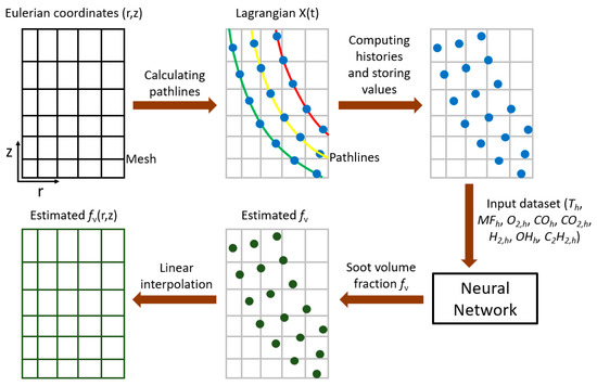
Figure 6.
A schematic representation of the ANN-based soot estimator approach.
Initially, all the ten input variables mentioned above were fed to the ANN. However, it was found that this would lead to the network finishing training within one iteration and thus returning extremely poor results. When this occurs, it is almost always indicative of an issue with the data or the network. Upon further investigation, it was determined that there were two variables, namely A1h and H2Oh, which when used in any combination with other variables would lead to the same issues. This behavior might be due to multicollinearity [45,46,47,48]. In fact, multicollinearity happens when the input variables are highly correlated (for instance, in the soot formation study, there is a strong correlation between C2H2,h and A1h) and they have a strong correlation with the output. In regression analysis, this may result in poor fitting [45,46,47,48]. In the current work, the two variables (A1h and H2Oh) were simply omitted from subsequent training of the network (it should be noted that from a physical perspective, it is not that A1h is not an important driver of aromatic growth and soot formation in this case, but rather that other input sets produce better results). Upon completion of some brief testing, it was determined that using all of the remaining eight variables as input parameters showed the most promise in terms of decreasing the overall error and improving reliability. It is important to emphasize again that these inputs were histories of variables as opposed to values in a given instant of time. This hysteresis method is necessary because the timescales associated with soot formation tend to be much longer than those of combustion chemistry. Furthermore, it should be noted that the concept of tracking the time history was also used by Aceves et al. [49] for fast prediction of HCCI combustion with an ANN linked to the KIVA3V fluid mechanics code. In addition, in the work of Christo et al. [28], in order to reduce the dependency of the ANN model on the selection of training sets for modeling turbulent flames, the input parameters were integrated over a prescribed reaction time.
As expected, an increase in runtime along with significantly improved results was realized with the additional input parameters when compared to the original three input variables (Th, MFh, H2,h) from previous work [18]. Furthermore, the repeatability of the results, where previously the exact same network would give largely varying results on several subsequent runs, was now much better. Nonetheless, variation will always be present to some degree, so it is a matter of limiting it as opposed to eliminating it. The reason this issue exists is the random nature behind the assignment of the initial weights paired with the random splitting of the entire data set into the training, validation, and testing sets (in this work, 80% of the entire dataset was randomly selected for training, 10% for validation, and 10% for testing). The randomness of the initial weights has a far smaller impact due to the fact that if the network works successfully it will always reach the global minimum. However, the data splitting does have a significant effect on the final results since the same network may be learning with different training data sets in successive runs, depending on how it is split. In this study, as an overall trend, the variability of these results decreased dramatically with the introduction of more input parameters.
From the onset of this study, there were some items of interest that were identified to have the potential to improve the performance of the ANN. Namely, these included data pre-processing, the number of input variables, the combination of input variables, the training method, the number of hidden layers and the number of neurons per hidden layer, and the activation function used.
As will be shown, data pre-processing had a considerable impact in this study. The results prior to the pre-processing were especially poor as they were not always physically realistic. Even though in the area where the flame is sooting the ANN returned fairly accurate results, the surrounding area where the soot volume fraction should be zero still had soot predicted for it. Not only was soot predicted there, but there were also regions of the predicted 2D field with negative concentrations. As negative values are unphysical, this was a very concerning result that had to be fixed if the estimators were to be of any use in the future.
The idea of data pre-processing was implemented in a work by Christo et al. [28]. In their study, a data pre-processing technique, called the histogram redistribution, was used to overcome the difficulties in achieving convergence of the network. This technique was based on using a nonlinear function, such as a natural logarithm, to transform the distorted or skewed distribution of the PDF into a more uniform one without changing the structure of the samples. Then, the transformed input datasets were used to train and test the neural network. Berger et al. [50] also suggested that taking the logarithm of the data before feeding it into the network significantly reduced errors when exploring data in a 3D or higher-dimensional space. After implementing the log transformation concept in the present study, significantly improved results were obtained. In the subsequent paragraphs, the process by which extensive fine-tuning of the network was completed is discussed. It is worth mentioning that several soot concentration predictions from the ANN with and without data pre-processing are presented in the results section.
The training method of an ANN refers to the actual method by which the weights and the biases of connections are adjusted during training. MATLAB R2018a allows for the selection of a variety of training methods [51]. For a given problem it is difficult to judge which training method will have the best performance without rigorous testing, as it is dependent on a concoction of factors, including the complexity of the problem, the number of data points, the number of weights and biases in the network, and many more. In this study, only two training methods were considered. The first method that was considered was the default method, called ‘Levenberg-Marquardt’ (which was explained in the methodology section) [25,26,52]. Additionally, the Scaled Conjugate Gradient (SCG) method [53] was also examined. This method is a class of conjugate gradient algorithms which are typically used for large-scale unconstrained optimization. However, since the theory behind this method is complex and beyond the scope of the present study, only the fundamentals are briefly discussed here. Consider the minimization of a function of variables. Conjugate gradient methods minimize this function with iterations of the form , where and are called the step length (always positive) and the search direction, respectively. It should be noted that if , the steepest descent method is obtained. While by assuming , the Newton algorithm is attained [54]. However, the SCG method proposed by Moller [53] is much more complicated. It is based on conjugate directions, but unlike other conjugate gradient methods, a line search at each iteration is not performed in this algorithm [53,55]. In the current study, the SCG was only brought into consideration due to the fact that if it were used as opposed to the Levenberg-Marquardt method, it would allow for the use of GPU (graphics processing unit) processing [51]. Since GPUs are effective at completing matrix mathematics, they prove to be extremely efficient for use in complex neural networks [56,57,58]. However, in our study, upon completing initial testing it was clear to see that the Scaled Conjugate Gradient gave far worse results which were not compensated for by the faster runtime. Therefore, the method was disregarded and further testing in the study was conducted with Levenberg-Marquardt training.
The last three parameters that were outlined to be tested initially were all done in tandem through the use of a grid search [59,60]. This technique essentially involves running through every possible combination of parameters to determine which single combination would give the best results. It should be pointed out that in general, manual search and grid search are the most extensively used approaches for hyper-parameter optimization. The major disadvantage of manual search is the fact that although a good result may be obtained, it is easy to miss the best result as only a select amount of combinations is considered. On the other hand, grid search suffers from the curse of dimensionality, as it quickly becomes too computationally-taxing to go through every single possibility for the network. However, in general, grid search is reliable in low dimensional spaces and typically results in a better configuration than would be obtained by purely manual sequential optimization in the same amount of time [61]. In the present study, 110 different combinations of the number of hidden layers and number of neurons per hidden layer were considered, along with two different activation functions (rectified linear unit and hyperbolic tangent). In fact, the number of hidden layers in the grid search was changed from 2 to 7, while the number of neurons per hidden layer was in the range of 3 to 25 (as demonstrated in the results, increasing the number of neurons causes the computational time to increase significantly. Consequently, the number of neurons per hidden layer was limited to 25). Additionally, each of the combinations was run five times to ensure repeatability. The main trends obtained from this study will be shown in the next section. Since the procedure was computationally expensive, parallel processing was used. The testing process utilized Compute Canada’s Niagara supercomputer and 40 CPUs. Using multiple clusters on Niagara allowed for several networks to be run concurrently as opposed to having to run one at a time. This allowed for far more testing to take place and ultimately helped in obtaining the final network architecture much faster than otherwise would have been possible.
3. Results and Discussion
Before going into detailed predictive results from the network, it is important to first examine the vast improvements associated with data pre-processing. This simple change in the network process led to the greatest advancement of the network’s predictive accuracy. As mentioned above, a detailed examination of the training dataset showed that the model accuracy and convergence depend on the nonuniformity and skewness in the distribution of the input dataset. A typical example is shown in Figure 7a for a highly skewed distribution of samples for the temporal history of oxygen (O2,h) before data pre-processing.
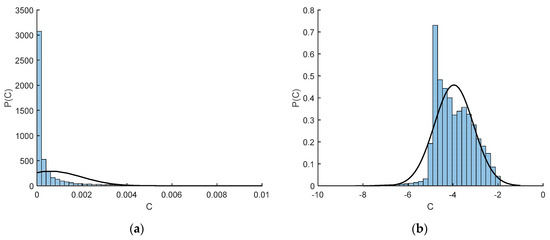
Figure 7.
The probability density function (PDF) of oxygen history (O2,h): (a) before data pre-processing; (b) after data pre-processing.
In statistical analyses, the data transformation concept is widely used to address skewed data [62]. Quite often data arising in real studies are far from the symmetric bell-shaped distribution and are so skewed that standard statistical analyses of these data become difficult and may yield inaccurate results [62]. Therefore, when the data distribution is non-normal and skewed, data transformations are utilized to make the data as ‘normal’ as possible [62]. The log transformation is the most common among the different kinds of data transformations [62,63]. Figure 7b shows that after using the log transformation in the present study, the data distribution (the histogram) has improved significantly and is closer to bell-shaped and resembles a normal distribution. Similar results were observed by Christo et al. [28]. For testing normality, the easiest approach is to compare the histograms to the normal probability curves (shown as solid lines in this figure). The log transformation was used here for the entire input set (since the data distribution of all the input variables were skewed), and then the transferred set was used as the training set for the neural network.
The results shown in Figure 8 depict the 2D soot volume fraction contours for the SY48 flame (see Table 1) obtained from the network with architecture of {8,5,3} (this notation means we have 3 hidden layers; 8 neurons in the first layer, 5 neurons in the second layer, and 3 neurons in the third layer (see Figure 1 for more information about the hidden layers)), eight inputs/one output (shown in Figure 6 and discussed in the previous section), and the tanh activation function. The stark difference between the results before and after the pre-processing was applied can be seen. Figure 8b highlights the poor results obtained without pre-processing when compared to the computed data (Figure 8a). As is experimentally known, only the flame and the area directly surrounding it can produce soot while the area outside of that has a soot volume fraction equal to zero. However, in Figure 8b there is soot predicted in the areas farther from the flame (notice the color difference between the computed and predicted figures). Furthermore, there are significant areas where the prediction is negative—something that is physically impossible. When examining Figure 8c, it is clear that these issues are no longer present, and the network is able to predict a soot volume fraction of zero where appropriate. However, it is important to note the apparent deterioration in results obtained in the sooting area in Figure 8c. Clearly, even though the overall results improved significantly (in terms of relative integrated error calculated over the entirety of the 2D field), the soot accuracy in the producing area suffered as a result, and thus the ensuing attempts at improving the network were focused on this region in particular.
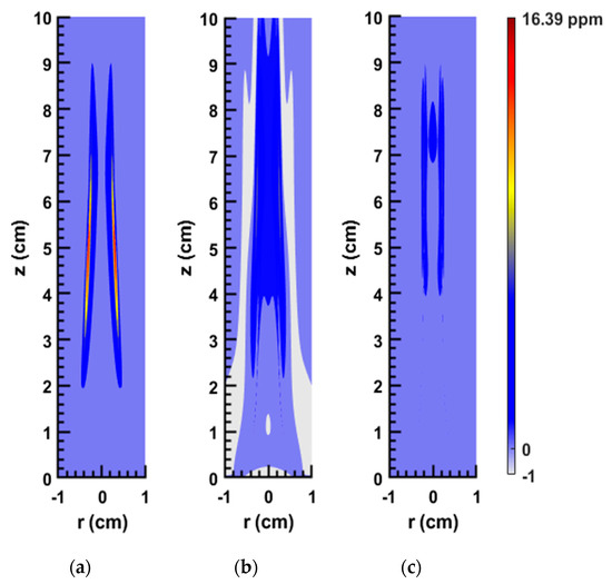
Figure 8.
2D contour plots of the soot volume fraction for the SY48 flame: (a) computed; (b) predicted by ANN without data pre-processing; (c) predicted by ANN with data pre-processing.
Aside from only examining particular results, it is imperative to look for overall trends that can be found in the grid search results. The grid search procedure reveals numerous trends in the results that can provide valuable information toward understanding these highly complex algorithms. The first trend that was observed is that calculations of complex architectures of several hidden layers and many neurons within each layer took significant runtime even with the parallelization in place. For instance, total run time (5 executions) for the networks with architectures of {15,15,15,15,15} (that is 5 hidden layers and 15 neurons within each layer), {15,15,15,15,15,15}, and {25,25,25} were 20.07, 27.45, and 47.08 h, respectively. In addition, the network predictions were often incorrect and unreliable, and the errors were extremely large. This is most likely due to the problem of overfitting where the model tunes itself so well to the training data that it no longer generalizes well to other data. In fact, deep neural networks make models more complex, and in a complex model it is more likely to have overfitting. Therefore, to develop a computationally efficient model (which is one of the main purposes of this study) and to prevent the problem of overfitting, shallower networks were focused on hereafter.
Furthermore, it was found that out of the two activation functions tested, the rectified linear unit gave far worse results when compared with the hyperbolic tangent. For instance, the average relative error of the peak fv (over 5 executions and based on the input/output datasets obtained from the eight flames in Table 1 (training errors)) for the networks with architectures of {15,10}, {10,5,3}, and {5,5,5,5} with the rectified linear unit activation function were 445.66, 1.3 × 10⁴ and 165.25%, respectively. However, by using the hyperbolic tangent activation function, the error for the mentioned architectures was reduced to 73.23, 139.28, and 42.58%, respectively. Similar trends were observed for other networks considered in the grid search. Therefore, only the hyperbolic tangent function was considered after this point.
As mentioned, a variety of architectures were tested, including some where the number of neurons in each layer remains the same and some where the number of neurons in each layer decreases with layer number, as if converging towards the output. It was found that networks with equal-numbered amounts of neurons in each layer were more consistent overall and delivered better results (for example, see the errors related to the networks with architectures of {15,10}, {10,5,3}, and {5,5,5,5} mentioned above). Similar observations were reported by Christo et al. [27] and de Villiers and Barnard [64]. In the work of Christo et al. [27], it was explained that substantial differences in the number of neurons result in a bottleneck junction of information so that the convergence of the algorithm is severely affected.
In the previous section, it was discussed that each network in our grid search was run five times to ensure repeatability. Overall, in this investigation, a lot of architectures showed good results for three or four out of the five runs. As an example, consider the network with the architecture of {10,5,3}. For this network, the relative errors of the peak fv for five executions were 15.21, 36.63, 16.98, 601.2, and 26.38% (average: 139.28%). As mentioned before, the variability is caused by the random splitting of the data into training/validation/testing subsets as well as random initialization of weights and biases. In the current study, a slightly higher error along with consistent results was preferred over a very low error occurring sporadically for the purpose of practical usability.
It is worth mentioning that, in the present study, to choose the optimal network architecture out of the 110 potential options, in addition to the analyses stated above (for instance, monitoring the network performance, the mean squared error, the relative error of the peak soot volume fraction () and the computational time), other errors such as the integrated relative errors were examined. The integrated represents the volumetric integration of the soot concentration in the whole domain and was calculated as [18]:
where provides quantification of the overall soot formation in the whole domain.
Upon analyzing all the results (eliminating networks with inconsistent results, large errors, and high computational cost), the final network that was chosen was the {10,10,10,10} (4 hidden layers and 10 neurons within each layer) since this network architecture exhibited excellent balance between runtime and performance. Its average error over five runs was 10.9%, peaking at 13.9% and going as low as 7.4%. When compared to the average error of 10.2% for the {10,10,10,10,10} architecture, the small decrease in error was accompanied by an increase in runtime of 0.9 h.
As stated in the introduction, the network was first trained with eight laminar flames and then used to predict the soot volume fraction for the exact same flames. This sort of evaluation is done to ensure that the network is able to accurately predict the flame characteristics for which it is trained. In addition to that test, two more rigorous tests were performed using two new datasets to check the ability of the network to predict the soot concentration for new laminar diffusion flames. As shown in Table 2, the first rigorous test is based on the experimental study of Santoro et al. [65] and the second one is based on the work of Cepeda et al. [66]. In order to perform these tests, Lagrangian fluid parcel tracking was employed with pre-computed CFD simulation data and the following histories were first calculated: Th, MFh, O2,h, COh, CO2,h, H2,h, OHh, and C2H2,h. Then, these eight parameters were used as input variables and the soot concentrations that were predicted by the network were compared with the CFD results.
Table 2.
The characteristics of two flames used as unseen data for the rigorous test (experimental work of a Santoro et al. [65]; experimental and numerical studies of b Cepeda et al. [66]).
The chosen network architecture ({10,10,10,10}) was run another five times, this time one at a time as opposed to consecutively, such that the error could be analyzed after every run instead of only at the end of the 5th one. This was done in search of the lowest possible error for the different tests mentioned above. Even though the network returns consistent results, there is still potential for it to have an even lower error due to the inherent variability present in the network predictions from run-to-run. It is worth mentioning that the runtime was approximately 50 min for a single training to complete and was done using four available cores on an average desktop computer through the use of MATLAB’s Parallel Computing Toolbox and the parpool function. This can be done much faster through the use of supercomputer clusters, but was timed on a regular workstation to act as a gauge for how long the typical user would have to run the tool.
At the end, one network which had the best performance among five trained networks for both tests mentioned above (namely, eight flames explained in Table 1 and two flames discussed in Table 2) was selected. Table 3 shows the relative errors in predicting soot concentration for all eight flames that were used to train this network. It includes the relative errors of integrated fv along the centerline and the streamline of maximum soot, the maximum fv, and the integrated fv in the whole domain. As shown, the average integrated soot volume fraction error over the whole domain is 8.08%.
Table 3.
Relative errors between the CFD and the predicted data by ANN for eight flames used to train the network.
Table 4, by contrast, shows the relative errors obtained from our rigorous tests for SA and CE flames using this network. As can be seen, for the SA flame, the relative errors are less than 20% and, in particular, the integrated fv error is 4.66%. However, for the CE flame, the errors are higher and the integrated fv error reaches 63.43%, mainly due to deviation of its dataset from the model’s dynamic range (similar observations were reported by Christo et al. [27] and Heinlein et al. [67]). For example, in the simulation of the CE flame, the fuel inlet velocity was assumed to be uniform and equal to 2.42 cm/s. For other nine flames discussed in the present work, the CFD results were based on the parabolic inlet velocity assumption and the minimum averaged fuel velocity was 4.1 cm/s (hence, the minimum fuel inlet velocity was 8.2 cm/s at the centerline, which was around 3.4 times more than the inlet velocity in the simulation of the CE flame). This degradation of accuracy, which occurs when the modelled samples are far enough outside the model’s working range, highlights the importance of broadening the training datasets to represent the input/output combinations over a wide dynamic range. It should be pointed out that the lack of data is one of the main reasons why machine-learning programs often fail to predict expected results [68]. Therefore, in future research, more flames will be simulated and validated, and more data will be added to the training dataset so that the network’s dynamic range will be expanded, making it the major advantage of this framework. It is worth mentioning that although more rigorous tests must be conducted to find the network performance, the range of errors for the CE flame is still very promising compared to many available CFD models that predict soot properties with about a one or two order-of-magnitude error.
Table 4.
Relative errors between the CFD and the predicted data by ANN for two flames used to test the network.
Figure 9, Figure 10 and Figure 11 demonstrate how our proposed network predicts the soot volume fraction (concentration) field for the eight flames stated in Table 1. To obtain these results, as explained in the methodology and demonstrated in Figure 6, the linear interpolation was performed. As shown in these figures, the network predicts the overall soot concentration field very well. The magnitude of the point of maximum soot is accurately predicted. All areas around the sooting region have a concentration value of zero. Furthermore, soot concentration distributions along the centerline and the streamline of maximum values are also properly estimated. It is worth mentioning that to keep the paper concise and to explain the details of the network predictions in different ways, 2D plots are presented for 4 flames (see Figure 9), and variations along the centerline and the streamline of maximum soot are revealed for the other 4 flames (see Figure 10 and Figure 11). These figures are discussed in more details in the following paragraphs.
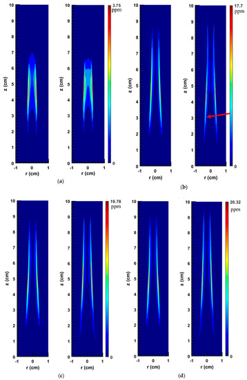
Figure 9.
2D soot concentration fields (ppm) for different flames: (a) SM80; (b) SY41; (c) SY46; (d) SY48; as obtained by two methods, using the original numerical solution (left image in each pair) and using the ANN prediction (right image in each pair).
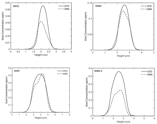
Figure 10.
Comparison of experimentally-validated CFD results and those obtained from the ANN for different flames along the centerline.
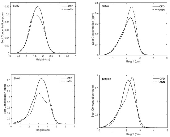
Figure 11.
Comparison of experimentally-validated CFD results and those obtained from the ANN for different flames along the streamline of maximum soot.
As shown in Figure 9a, for the flame SM80, the shape of the soot field is accurately captured by the ANN prediction. However, compared to the original case, the high-soot zone predicted by the ANN is slightly longer and thicker. Near the centerline when the distance from the burner exit is between 4.8 and 6 cm, the discrepancy is more noticeable. At the centerline, the maximum soot values are 1.176 and 1.038 ppm for the ANN and the original cases, respectively. In addition, the peak soot values in the entire domain are 3.75 and 3.21 ppm (see Table 1) for the ANN and the original cases, respectively.
Figure 9b shows the soot volume fraction fields for the SY41 flame. In general, the ANN prediction is in good agreement with the CFD results. The sooting region predicted by the ANN is slightly longer in comparison with the original case. However, the high-soot zone (where soot is more than 6 ppm) estimated by the network is slightly shorter and thinner. Moreover, as shown, fv predicted by the network reaches a peak at 17.70 ppm, while the original fv obtained from CFD peaks at 12.65 ppm (see Table 1). To present more details, it should be pointed out that, at the centerline, the soot volume fraction peaks at 1.96 and 1.91 ppm for the original and the ANN cases, respectively. In addition, there are slight and insignificant fluctuations in the ANN prediction when z is between 1.5 and 3 cm (see the red arrow in Figure 9b). It only happens in a limited small area at the boundary of the soot domain and can be due to the overfitting problem. Attempts were made to eliminate these fluctuations by changing our network architecture, but were unsuccessful.
In Figure 9c the soot volume fraction fields for the SY46 flame are shown. As can be seen, the length of sooting region predicted by the network is 20% greater than that obtained from the CoFlame code. In addition, the length of the high-soot concentration zone (where soot is more than 6 ppm) estimated by the network is 23% longer and 6% thicker. In this figure, the fluctuations in the ANN prediction at the boundary of the soot domain when z is between 1.4 and 3.2 cm are also visible. Additionally, the maximum fv predicted by the network and calculated by the CoFlame code are 19.78 and 14.76 ppm, respectively. For the fv along the centerline, the relative error is only 3.85% in this case.
The original and ANN predicted soot volume fraction fields for the SY48 flame are shown in Figure 9d. As illustrated, both the length of the soot domain (non-zero values) and the length of the high-soot zone (where soot is more than 8 ppm) predicted by the network are greater compared to the original cases. Meanwhile, the thickness of high-soot zone is almost the same. Moreover, the fv reaches a peak at 20.32 and 16.39 ppm for the ANN and the original cases, respectively. In this figure, slight fluctuations in the ANN prediction when z is between 1.5 and 3.5 cm are also present.
Figure 10 and Figure 11 show the variations of soot volume fraction along the centerline and the streamline of maximum soot for flames SM32, SM40, SM60, and SM80.2. The predictions of the proposed network as well as the CFD results are plotted. As can be seen, in general, there is very good agreement between the ANN and the CFD results and the trends of changes are accurately captured. However, it is worth mentioning that for the SM32 flame, in general, the network underestimates the soot concentration along the centerline and the streamline of maximum soot. A different tendency can be seen in SM40 flame, where the network underestimates and overestimates fv along the centerline and along the streamline of maximum soot, respectively. For the SM60 flame, the network underestimates the soot concentration along the streamline of maximum soot, while it shows very good prediction along the centerline. Conversely, for the SM80.2 flame, the network underestimates the soot concentration along the centerline, while its prediction along the streamline of maximum soot is slightly shifted compared with the CFD results.
Figure 12, Figure 13, Figure 14 and Figure 15 reveal the results of a more rigorous test, wherein the network was used to predict the soot concentration for SA and CE flames mentioned in Table 2. As can be seen, the network predicts the overall soot field for the SA flame very well. However, as stated above, the error is higher for the CE flame. In Figure 12, it is shown that for the SA flame, by using the proposed network, fv reaches a peak of 12.85 ppm and the high-soot zone becomes shorter than the same respective area in the 2D plot obtained from the numerical solution of the flame. It should be noted that in the CFD results, the maximum fv for SA flame is equal to 10.74 ppm. In addition, as shown in Figure 14 and Figure 15, the network predicts the soot concentration for the SA flame along the centerline and the streamline of maximum soot with only a slight discrepancy.
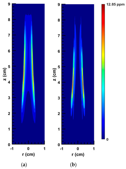
Figure 12.
2D soot concentration field of the SA flame: (a) original numerical solution; (b) ANN prediction.
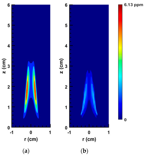
Figure 13.
2D soot concentration field of the CE flame: (a) original numerical solution; (b) ANN prediction.
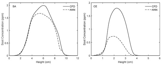
Figure 14.
Comparison of experimentally-validated CFD results and those obtained from the ANN along the centerline for the flames used to test the network.
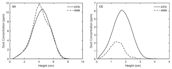
Figure 15.
Comparison of experimentally-validated CFD results and those obtained from the ANN along the streamline of maximum soot for the flames used to test the network.
Figure 13 shows that although our network is able to predict the soot zone size and shape for the CE flame accurately, the values of fv are underestimated. As shown, based on the network results, the fv peaks at 2.9 ppm. However, the maximum value of fv according to our CFD results is 6.13 ppm. Figure 14 and Figure 15 also demonstrate that the network underestimates the soot concentration for the CE flame along the centerline and the streamline of maximum soot (the values of relative errors are reported in Table 4). As mentioned above, this degradation in performance happens if the modelled compositions deviate significantly from the network’s working range.
All the errors mentioned above are relative because the range of fv in this study is wide, from around 0.1 to 20 ppm. In general, for the flames with low fv the absolute error was also very low (for example around ). Conversely, the flames with high fv had absolute errors in the order of magnitude of 1. To display the graphs of absolute error in an easy-to-read way, the following equation was developed firstly:
In the above equation, the error is a function of z (height) only, due to averaging in the radial direction. It is worth mentioning that taking the average of soot volume fraction over one direction (here r direction) reduces the error fluctuations significantly and makes the error behavior more obvious without obfuscating it. The domain was chosen since it covers all the soot regions in all the ten flames discussed above. Figure 16a shows the results obtained from the above equation for the flames SM32, SY48, SA, and CE. As can be seen, for the flame SM32, the error reaches a peak of around while for the other three flames the maximum error is slightly less than 1 (noting that the scale of the vertical axis is logarithmic). However, as shown in Table 1 and Table 2, the peak fv for these flames are 0.12, 16.39, 10.74, and 6.13, respectively. By normalizing the error graphs with the peak fv, the percentage of error can be obtained:
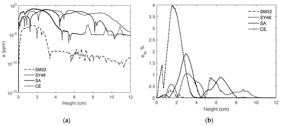
Figure 16.
The variations of average error versus height: (a) absolute error; (b) absolute error normalized with the peak soot volume fraction.
Figure 16b shows the variations of versus height. As demonstrated, when z is less than 4 cm, the CE flame has the highest error among these flames (this was shown in Figure 13 and was discussed above comprehensively). For the SA and SY48 flames, fluctuates more but is less than 2%. For the SM32 flame, the normalized error is clearly less than 0.5%. It should be pointed out that, to analyse the soot estimator concept, different types of errors, especially relative errors (similar to the errors defined in this study), must be used because the problem is challenging, and the range of the soot concentration and the number of the flames are vast.
4. Conclusions and Future Works
In this study, a supervised Artificial Neural Network (ANN) technique was used to accurately estimate the soot concentration fields in laminar diffusion flames. Eight different ethylene/air flames at various operating conditions were modeled using the CoFlame code. Then, the Lagrangian histories of soot-containing fluid parcels were considered as the input dataset. The effects of data pre-processing, number of input parameters, random splitting, and training method on the network performance and results were discussed. A grid search procedure was used to study the effects of the number of hidden layers, number of neurons, and the activation functions. In conclusion, the {10,10,10,10} network architecture together with eight input parameters, the Levenberg-Marquardt training method, and the hyperbolic tangent activation function were identified as the most effective framework.
The resulting network was tested in two different ways: (1) it was applied to predict the soot volume fraction for all eight flames that were used in the training phase; (2) two new flames were then introduced to the network and its predictions were analyzed. In general, the network predicts the overall soot field accurately and efficiently. However, some degradation in the accuracy becomes noticeable once the datasets deviate significantly from the network’s dynamic range. It is also shown in this study that the ANN approach scales extremely well to added dimensions, which is an important step for exploring more complex cases such as transient and turbulent sooting flames (where timescales of the data are much larger). Overall, this study demonstrates the potential of the soot estimator to be implemented through the use of neural networks.
In machine learning, the accuracy of the predictions is related to how close the target properties are to the training datasets. To improve the estimator’s predictions and test the network at different conditions, more flames should be simulated using the CoFlame code and validated against experimental measurements. In this case, the training and testing datasets are expanded so that the issue of the lack of data can be resolved and the network’s dynamic range can be developed. In addition, it is intended for the next step to use the estimator tool for predicting soot characteristics in transient and turbulent flames. In the next step, similar to the concept presented in the present study, machine-learning and deep-learning programs will be used as post-processing tools to estimate the soot characteristics based on the soot-related gas-phase quantities obtained from Reynolds-averaged Navier-Stokes (RANS), large eddy simulation (LES), and direct numerical simulation (DNS) solutions. Afterwards, this approach can be applied to estimate the soot characteristics in complicated industrial cases such as an actual engine. In this case, the industrial sector would have an accurate and computationally inexpensive tool in which only the gas-phase conservation equations (which are typically solved in any combustion simulation) need to be solved. In short, the tool would take advantage of detailed soot formation models with no need to solve the soot partial differential equations as well as different soot-related terms such as soot particle nucleation, coagulation, PAH condensation, HACA surface growth, oxidation, and fragmentation, since all of them are replaced with an ANN.
Author Contributions
Conceptualization, S.B.D. and L.Z.; methodology, M.J., S.K. and L.Z.; software, M.J., S.K. and L.Z.; writing—original draft preparation, M.J. and S.K.; writing—review and editing, S.B.D.; supervision, S.B.D. All authors have read and agreed to the published version of the manuscript.
Funding
This research received no external funding.
Acknowledgments
The authors acknowledge funding from the Canadian Research Chairs Program and the Natural Sciences and Engineering Research Council (NSERC).
Conflicts of Interest
The authors declare no conflict of interest.
References
- Center for American Progress. Soot Pollution. Available online: https://www.americanprogress.org/issues/green/news/2012/08/10/12007/soot-pollution-101/ (accessed on 7 September 2020).
- Environmental Protection Agency. Particulate Matter (PM) Basics. Available online: https://www.epa.gov/pm-pollution (accessed on 7 September 2020).
- Lighty, J.A.S.; Veranth, J.M.; Sarofim, A.F. Combustion aerosols: Factors governing their size and composition and implications to human health. J. Air Waste Manag. Assoc. 2000, 50, 1565–1618. [Google Scholar] [CrossRef] [PubMed]
- Jacobson, M.Z. Strong radiative heating due to the mixing state of black carbon in atmospheric aerosols. Nature 2001, 409, 695–697. [Google Scholar] [CrossRef] [PubMed]
- Williams, M.; Minjares, R. A Technical Summary of Euro 6/VI Vehicle Emission Standards. Int. Counc. Clean Transp. Brief. Pap. 2016. Available online: https://theicct.org/publications/technical-summary-euro-6vi-vehicle-emission-standards (accessed on 7 September 2020).
- Alexander, R.; Bozorgzadeh, S.; Khosousi, A.; Dworkin, S.B. Development and testing of a soot particle concentration estimator using lagrangian post-processing. Eng. Appl. Comput. Fluid Mech. 2018, 12, 236–249. [Google Scholar] [CrossRef]
- Mueller, M.E.; Pitsch, H. LES model for sooting turbulent nonpremixed flames. Combust. Flame 2012, 159, 2166–2180. [Google Scholar] [CrossRef]
- Han, W.; Raman, V.; Mueller, M.E.; Chen, Z. Effects of combustion models on soot formation and evolution in turbulent nonpremixed flames. Proc. Combust. Inst. 2019, 37, 985–992. [Google Scholar] [CrossRef]
- Brocklehurst, H.T.; Priddin, C.H.; Moss, J.B. Soot predictions within an aero gas turbine combustion chamber. In Proceedings of the ASME Turbo Expo, Orlando, FL, USA, 2–5 June 1997. [Google Scholar] [CrossRef]
- Tolpadi, A.K.; Danis, A.M.; Mongia, H.C.; Lindstedt, R.P. Soot Modeling in Gas Turbine Combustors. In Proceedings of the ASME Turbo Expo, Orlando, FL, USA, 2–5 June 1997. [Google Scholar] [CrossRef]
- Mueller, M.E.; Pitsch, H. Large eddy simulation of soot evolution in an aircraft combustor. Phys. Fluids 2013, 25, 110812. [Google Scholar] [CrossRef]
- Eaves, N.A.; Zhang, Q.; Liu, F.; Guo, H.; Dworkin, S.B.; Thomson, M.J. CoFlame: A refined and validated numerical algorithm for modeling sooting laminar coflow diffusion flames. Comput. Phys. Commun. 2016, 207, 464–477. [Google Scholar] [CrossRef]
- Mueller, M.E.; Blanquart, G.; Pitsch, H. Hybrid Method of Moments for modeling soot formation and growth. Combust. Flame 2009, 156, 1143–1155. [Google Scholar] [CrossRef]
- Bisetti, F.; Blanquart, G.; Mueller, M.E.; Pitsch, H. On the formation and early evolution of soot in turbulent nonpremixed flames. Combust. Flame 2012, 159, 317–335. [Google Scholar] [CrossRef]
- Attili, A.; Bisetti, F.; Mueller, M.E.; Pitsch, H. Formation, growth, and transport of soot in a three-dimensional turbulent non-premixed jet flame. Combust. Flame 2014, 161, 1849–1865. [Google Scholar] [CrossRef]
- Wick, A.; Attili, A.; Bisetti, F.; Pitsch, H. DNS-driven analysis of the Flamelet/Progress Variable model assumptions on soot inception, growth, and oxidation in turbulent flames. Combust. Flame 2020, 214, 437–449. [Google Scholar] [CrossRef]
- Zimmer, L.; Dworkin, S.B.; Attili, A.; Pitsch, H.; Bisetti, F. A soot particle concentration estimator applied to a transient turbulent non-premixed jet flame. In Proceedings of the Combustion Institute—Canadian Section Spring Technical Meeting, Kelowna, BC, Canada, 13–16 May 2019. [Google Scholar]
- Zimmer, L.; Kostic, S.; Dworkin, S.B. A novel soot concentration field estimator applied to sooting ethylene/air laminar flames. Eng. Appl. Comput. Fluid Mech. 2019, 13, 470–481. [Google Scholar] [CrossRef]
- Bozorgzadeh, S. Development of a Soot Concentration Estimator for Industrial Combustion Applications. Master’s Thesis, Ryerson University, Toronto, ON, Canada, 2014. [Google Scholar]
- Veshkini, A.; Dworkin, S.B.; Thomson, M.J. A soot particle surface reactivity model applied to a wide range of laminar ethylene/air flames. Combust. Flame 2014, 161, 3191–3200. [Google Scholar] [CrossRef]
- Kholghy, M.R.; Veshkini, A.; Thomson, M.J. The core-shell internal nanostructure of soot—A criterion to model soot maturity. Carbon 2016, 100, 508–536. [Google Scholar] [CrossRef]
- Nielsen, M. Neural Networks and Deep Learning. Available online: http://neuralnetworksanddeeplearning.com/ (accessed on 7 September 2020).
- Wang, Y.; Li, Y.; Song, Y.; Rong, X. The influence of the activation function in a convolution neural network model of facial expression recognition. Appl. Sci. 2020, 10, 1897. [Google Scholar] [CrossRef]
- Liu, Q.; Wu, Y. Supervised Learning. In Encyclopedia of the Sciences of Learning; Springer: Boston, MA, USA, 2012; pp. 3243–3245. [Google Scholar]
- The Mathworks Inc. Levenberg-Marquardt Backpropagation. Available online: https://www.mathworks.com/help/deeplearning/ref/trainlm.html (accessed on 7 September 2020).
- Yu, H.; Wilamowski, B.M. Levenberg-marquardt training. In Intelligent Systems; CRC Press: Boca Raton, FL, USA, 2011; pp. 1–16. [Google Scholar]
- Christo, F.C.; Masri, A.R.; Nebot, E.M.; Turanyi, T. Utilizing artificial neural network and repro-modelling in turbulent combustion. In Proceedings of the ICNN’95—IEEE International Conference on Neural Networks, Perth, WA, Australia, 27 November–1 December 1995; pp. 911–916. [Google Scholar] [CrossRef]
- Christo, F.C.; Masri, A.R.; Nebot, E.M.; Pope, S.B. An integrated PDF/neural network approach for simulating turbulent reacting systems. Symp. Int. Combust. 1996, 26, 43–48. [Google Scholar] [CrossRef]
- Li, S.; Yang, B.; Qi, F. Accelerate global sensitivity analysis using artificial neural network algorithm: Case studies for combustion kinetic model. Combust. Flame 2016, 168, 53–64. [Google Scholar] [CrossRef]
- Christo, F.C.; Masri, A.R.; Nebot, E.M. Artificial neural network implementation of chemistry with pdf simulation of H2/CO2 flames. Combust. Flame 1996, 106, 406–427. [Google Scholar] [CrossRef]
- Blasco, J.A.; Fueyo, N.; Dopazo, C.; Ballester, J. Modelling the temporal evolution of a reduced combustion chemical system with an artificial neural network. Combust. Flame 1998, 113, 38–52. [Google Scholar] [CrossRef]
- Blasco, J.A.; Fueyo, N.; Larroya, J.C.; Dopazo, C.; Chen, Y.J. A single-step time-integrator of a methane-air chemical system using artificial neural networks. Comput. Chem. Eng. 1999, 23, 1127–1133. [Google Scholar] [CrossRef]
- Ihme, M.; Schmitt, C.; Pitsch, H. Optimal artificial neural networks and tabulation methods for chemistry representation in les of a bluff-body swirl-stabilized flame. Proc. Combust. Inst. 2009, 32, 1527–1535. [Google Scholar] [CrossRef]
- Pulga, L.; Bianchi, G.M.; Falfari, S.; Forte, C. A machine learning methodology for improving the accuracy of laminar flame simulations with reduced chemical kinetics mechanisms. Combust. Flame 2020, 216, 72–81. [Google Scholar] [CrossRef]
- Ranade, R.; Li, G.; Li, S.; Echekki, T. An Efficient Machine-Learning Approach for PDF Tabulation in Turbulent Combustion Closure. Combust. Sci. Technol. 2019. [Google Scholar] [CrossRef]
- Ranade, R.; Alqahtani, S.; Farooq, A.; Echekki, T. An ANN based hybrid chemistry framework for complex fuels. Fuel 2019, 241, 625–636. [Google Scholar] [CrossRef]
- Emami, M.D.; Eshghinejad Fard, A. Laminar flamelet modeling of a turbulent CH4/H2/N2 jet diffusion flame using artificial neural networks. Appl. Math. Model. 2012, 36, 2082–2093. [Google Scholar] [CrossRef]
- Inal, F.; Tayfur, G.; Melton, T.R.; Senkan, S.M. Experimental and artificial neural network modeling study on soot formation in premixed hydrocarbon flames. Fuel 2003, 82, 1477–1490. [Google Scholar] [CrossRef]
- Inal, F. Artificial neural network predictions of polycyclic aromatic hydrocarbon formation in premixed n-heptane flames. Fuel Process. Technol. 2006, 87, 1031–1036. [Google Scholar] [CrossRef]
- Eaves, N.A.; Thomson, M.J.; Dworkin, S.B. The Effect of Conjugate Heat Transfer on Soot Formation Modeling at Elevated Pressures. Combust. Sci. Technol. 2013, 185, 1799–1819. [Google Scholar] [CrossRef]
- Veshkini, A.; Dworkin, S.B. A computational study of soot formation and flame structure of coflow laminar methane/air diffusion flames under microgravity and normal gravity. Combust. Theory Model. 2017, 21, 864–878. [Google Scholar] [CrossRef]
- Mansouri, A.; Eaves, N.A.; Thomson, M.J.; Dworkin, S.B. Influence of pressure on near nozzle flow field and soot formation in laminar co-flow diffusion flames. Combust. Theory Model. 2019, 23, 536–548. [Google Scholar] [CrossRef]
- Smooke, M.D.; Long, M.B.; Connelly, B.C.; Colket, M.B.; Hall, R.J. Soot formation in laminar diffusion flames. Combust. Flame 2005, 143, 613–628. [Google Scholar] [CrossRef]
- Shaddix, C.R.; Smyth, K.C. Laser-induced incandescence measurements of soot production in steady and flickering methane, propane, and ethylene diffusion flames. Combust. Flame 1996, 107, 418–452. [Google Scholar] [CrossRef]
- Farrar, D.E.; Glauber, R.R. Multicollinearity in Regression Analysis: The Problem Revisited. Rev. Econ. Stat. 1967, 49, 92–107. [Google Scholar] [CrossRef]
- Allen, M.P. Understanding Regression Analysis; Springer: Boston, MA, USA, 2007; pp. 176–180. [Google Scholar]
- RYAN, T.P. Modern Regression Methods; John Wiley & Sons, Inc.: Hoboken, NJ, USA, 2008. [Google Scholar]
- Chatterjee, S.; Hadi, A.S. Regression Analysis by Example; John Wiley & Sons, Inc.: Hoboken, NJ, USA, 2006. [Google Scholar]
- Aceves, S.M.; Flowers, D.L.; Chen, J.Y.; Babajimopoulos, A. Fast Prediction of HCCIcombustion with an Artificial Neural Network Linked to a Fluid Mechanics Code; SAE: Warrendale, PA, USA, 2006. [Google Scholar] [CrossRef]
- Berger, L.; Kleinheinz, K.; Attili, A.; Bisetti, F.; Pitsch, H.; Mueller, M.E. Numerically accurate computational techniques for optimal estimator analyses of multi-parameter models. Combust. Theory Model. 2018, 22, 480–504. [Google Scholar] [CrossRef]
- The Mathworks Inc. MATLAB R2018a. Available online: www.mathworks.com/products/matlab (accessed on 7 September 2020).
- Hagan, M.T.; Menhaj, M.B. Training Feedforward Networks with the Marquardt Algorithm. IEEE Trans. Neural Netw. 1994, 5, 989–993. [Google Scholar] [CrossRef] [PubMed]
- Møller, M.F. A scaled conjugate gradient algorithm for fast supervised learning. Neural Netw. 1993, 6, 525–533. [Google Scholar] [CrossRef]
- Andrei, N. Conjugate gradient algorithms for molecular formation under pairwise potential minimization. In Proceedings of the Fifth Workshop on Mathematical Modelling of Environmental and Life Sciences Problems, Constanta, Romania, 10–13 September 2006; pp. 7–26. [Google Scholar]
- The Mathworks Inc. Scaled Conjugate Gradient Backpropagation. Available online: https://www.mathworks.com/help/deeplearning/ref/trainscg.html (accessed on 4 September 2020).
- Memon, Z.A.; Samad, F.; Awan, Z.R.; Aziz, A.; Siddiqi, S.S. CPU-GPU processing. Int. J. Comput. Sci. Netw. Secur. 2017, 17, 188–193. [Google Scholar]
- Lind, E.; Pantigoso, A. A Performance Comparison between CPU and GPU in TensorFlow. Bachelor’s Thesis, KTH Royal Institute of Technology, Stockholm, Sweden, 2019. [Google Scholar]
- Schlegel, D. Deep Machine Learning on GPUs; Seminar Talk, Computer Engineering Group; University of Heidelberg: Heidelberg, Germany, 2015. [Google Scholar]
- Hsu, W.; Chang, C.C.; Lin, C.J. A Practical Guide to Support Vector Classification; Technical Report; Department of Computer Science, National Taiwan University: Taipei, Taiwan, 2003. [Google Scholar]
- Chicco, D. Ten quick tips for machine learning in computational biology. BioData Min. 2017, 10, 35. [Google Scholar] [CrossRef]
- Bergstra, J.; Bengio, Y. Random search for hyper-parameter optimization. J. Mach. Learn. Res. 2012, 13, 281–305. [Google Scholar]
- Feng, C.; Wang, H.; Lu, N.; Chen, T.; He, H.; Lu, Y.; Tu, X.M. Log-transformation and its implications for data analysis. Shanghai Arch. Psychiatry 2014, 26, 105–109. [Google Scholar] [CrossRef]
- Feng, C.; Wang, H.; Lu, N.; Tu, X.M. Log transformation: Application and interpretation in biomedical research. Stat. Med. 2013, 32, 230–239. [Google Scholar] [CrossRef] [PubMed]
- de Villiers, J.; Barnard, E. Backpropagation Neural Nets with One and Two Hidden Layers. IEEE Trans. Neural Netw. 1993, 4, 136–141. [Google Scholar] [CrossRef] [PubMed]
- Santoro, R.J.; Semerjian, H.G.; Dobbins, R.A. Soot particle measurements in diffusion flames. Combust. Flame 1983, 51, 203–218. [Google Scholar] [CrossRef]
- Cepeda, F.; Jerez, A.; Demarco, R.; Liu, F.; Fuentes, A. Influence of water-vapor in oxidizer stream on the sooting behavior for laminar coflow ethylene diffusion flames. Combust. Flame 2019, 210, 114–125. [Google Scholar] [CrossRef]
- Heinlein, J.; Schulte, G.; Fritsching, U.; Guardani, R. Mapping the structure of a liquid spray by means of neural networks. Chem. Eng. Process. Process Intensif. 2007, 46, 1357–1364. [Google Scholar] [CrossRef]
- Machine Learning. Available online: https://en.wikipedia.org/wiki/Machine_learning (accessed on 7 September 2020).


© 2020 by the authors. Licensee MDPI, Basel, Switzerland. This article is an open access article distributed under the terms and conditions of the Creative Commons Attribution (CC BY) license (http://creativecommons.org/licenses/by/4.0/).