Article

Multi-Agent Cooperation Based Reduced-Dimension Q(λ) Learning for Optimal Carbon-Energy Combined-Flow

1
Power Grid Planning Center of Guangdong Power Grid Co., Ltd., Guangzhou 510640, China
2
School of Electric Power, South China University of Technology, Guangzhou 510640, China
*
Author to whom correspondence should be addressed.
Energies 2020, 13(18), 4778; https://doi.org/10.3390/en13184778
Submission received: 17 June 2020 / Revised: 27 August 2020 / Accepted: 31 August 2020 / Published: 14 September 2020
(This article belongs to the Special Issue Enhancement of Industrial Energy Efficiency and Sustainability)

Abstract

:
This paper builds an optimal carbon-energy combined-flow (OCECF) model to optimize the carbon emission and energy losses of power grids simultaneously. A novel multi-agent cooperative reduced-dimension Q(λ) (MCR-Q(λ)) is proposed for solving the model. Firstly, on the basis of the traditional single-objective Q(λ) algorithm, the solution space is reduced effectively to shrink the size of Q-value matrices. Then, based on the concept of ant cooperative cooperation, multi-agents are used to update the Q-value matrices iteratively, which can significantly improve the updating rate. The simulation in the IEEE 118-bus system indicates that the proposed technique can decrease the convergence speed by hundreds of times as compared with conventional Q(λ), keeping high global stability, which is very suitable for dynamic OCECF in a large and complex power grid compared with other algorithms.

Graphical Abstract

1. Introduction

With the increasing impact of the greenhouse effect on the environment, low-carbon economy has gradually become the key development direction of various energy consumption industries. As the largest CO2 emitter, the electric power industry will play an important role in low-carbon economic development [1]. All kinds of energy-consuming enterprises have also commenced on focusing on the control of carbon emissions, especially in the power industry, which makes up approximately 40% of CO2 emissions in the whole world [2]. Generally speaking, low-carbon power involves four sectors: generation, transmission, distribution and consumption. Therefore, how to reduce the carbon emissions of transmission and distribution sectors in the power grid industry has turned into an instant issue to be solved [3,4].
Up to now, numerous scholars have carried out research on all aspects of low-carbon power, including optimal power flow (OPF) [5,6,7], economic emission dispatching [8,9], low-carbon power system dispatch [10], unit commitment [11,12], carbon storage and capture [13,14] and other issues. However, the previous studies mainly focused on the carbon emissions of the generation side, with a lack of research on how to reduce the carbon emissions of the power network (i.e., the transmission and distribution sides). Therefore, the optimal carbon-energy combined-flow (OCECF) model, which can reflect the energy flow and carbon flow distribution of the power grid, is further established in this paper. Basically, the OCECF is on the basis of the conventional reactive power optimization model, which should not only attempt to minimize the power loss and voltage deviation, but also aim to minimize the carbon emission of the power network while satisfying the various operating constraints of power systems.
Obviously, the OCECF is a complicated nonlinear planning problem considering the carbon flow losses of power grids, which can be solved by traditional optimization strategies including nonlinear planning [15], the Newton method [16] and the interior point method [17]. However, due to the strong nonlinearity of power systems, the discontinuity of the objective function and constraint conditions, as well as the existence of multiple local optimal solutions, usually hinder the effectiveness or applications of the classical optimization methods. On the other hand, meta-heuristic algorithms including the genetic algorithm (GA) [18], particle swarm optimization (PSO) [19,20], grouped grey wolf optimizer (GWO) [21] and the memetic salp swarm algorithm (MSSA) [22] have relatively low dependence on specific models, and can obtain relatively satisfactory results when solving such problems. However, due to the low convergence stability of the algorithm, these algorithms may only converge to a local optimal solution. Thus, the conventional Q(λ) reinforcement learning algorithm with better convergence robustness and stability is proposed in [23]. Nevertheless, because of the search ergodicity of the single agent Q(λ) algorithm, its convergence is relatively long for large-scale system optimization due to the low learning efficiency, while the “dimension disaster” problem with the increasing number of variables can also occur. Moreover, the on-line optimization requirement of the OCECF is also difficult to be met.
Therefore, the author of ant colony optimization (ACO) introduces the concept of ant colony in the classical Q-learning algorithm and puts forward the multiagent Ant-Q algorithm with a faster optimization speed [24]. Based on this, a new multi-agent cooperation-based reduced-dimension Q(λ) (MCR-Q(λ)) learning is proposed for OCECE in this paper, which mainly contains the following contributions:
(i) Most of existing low-carbon power studies did not consider the carbon emissions of the power network due to the energy flow and carbon flow from the generation side to the load side, which cannot satisfy the low-carbon requirement from the viewpoint of the power network. In contrast, the presented OCECF can further reduce the carbon emissions of the power network, which can improve the benefit of the power grid company in a carbon trading market.
(ii) The proposed MCR-Q(λ) can effectively shorten the dimension of the solution space of the Q algorithm to solve the OCECF problem by introducing the eligibility trace (λ) returns mechanism [23]. Besides, it also can accelerate the convergence rate and avoid trapping into a low-quality optimum for OCECE via multi-agent cooperation.
The framework of this paper mainly includes: firstly, Section 2 which concludes the related work; Section 3 presents the establishment of the OCECF mathematical model; then, the principle of MCR-Q(λ) learning is described in Section 4; Section 5 gives the concrete steps of solving the OCECF problem; Section 6 undertakes simulation studies on the IEEE 118 node system to verify the convergence and stability of MCR-Q(λ) learning. Finally, the conclusion of the whole paper is presented in Section 7.

2. Related Work

2.1. Low-Carbon Power

To achieve a low-carbon operation of a power system, extensive studies were devoted to addressing the environmental economic dispatch (EED). In EED, the minimization of emissions [25] is generally designed as one part of the objective function. To further improve the operation economy, the uncertainty of wind power was considered in [26,27], in which the power output of a wind turbine was evaluated based on a probability distribution function of the wind speed. Besides, a modified EED, by combining heat and power economic dispatch, was presented in [28], which can achieve an optimal operation for the heat and power system simultaneously. Furthermore, a coordinated operation of an integrated regional energy system with various energies (e.g., a CO2-capture-based power) was proposed in [29], while the demand response was also introduced in EED. To further reduce carbon emissions, the CO2 emission trading system was combined into the daily operation of an energy system. In [30], a decentralized economic dispatch was proposed by considering the carbon capture power plants with carbon emission trading. Moreover, the power uncertainty of wind and photovoltaic energy was fully taken into account in [31,32] based on carbon emission trading. For the purpose of clarifying the internal relation between energy consumption and carbon emissions from power grids, the concept of carbon emission flow is put forward for the first time in reference [33]. On this basis, the authors of [34,35,36] carried out a theoretical analysis and case verification on the carbon emission flow calculation and the carbon flow tracking of a power system, respectively.

2.2. Application of Meta-Heuristic Algorithms

In fact, the optimal low-carbon operation of a power system faces with various complex and difficult optimization problems, e.g., EED. Hence, various meta-heuristic algorithms have been employed for these optimization problems due to their strong searching ability and high application flexibility. In [25], an improved PSO combining the differential evolution algorithms was designed for EED. In [26], a so-called exchange market algorithm was used for EED due to its fast convergence and strong global searching ability. In [27], a population-based honey bee mating optimization with an online learning mechanism was presented. Inspired by the well-known tag-team game in India, the novel Kho-Kho optimization algorithm [28] with an excellent optimization performance was proposed for EED. To achieve a distributed optimization for real-time power dispatch, a novel adaptive distributed auction-based algorithm with a varying swap size was proposed in [37]. On the other hand, the reinforcement learning-based optimization attracted many investigations for optimal operations of power systems. In [23], a distributed multi-step Q(λ) learning was proposed for the complex OPF of a large-scale power system. To satisfy the requirement of multi-objective optimization, an approximate ideal multi-objective solution Q(λ) learning was presented in [36] via a design of multiple Q matrices for different objective functions.

3. OCECF Mathematical Model

3.1. Carbon-Energy Combined-Flow

The carbon-energy combined-flow (CECF) of the power grid is a comprehensive network flow [36], which combines the power flow of the power grid with the carbon emission flow attached to the power flow of the power grid. Among them, the energy flow is the actual network flow, and the carbon emission flow is the virtual network flow, which can be referred to as the carbon flow in the power system. Carbon flow is generated in the power generation, which represents the concept that the carbon emission is transferred from the generation side to the demand side. The energy flow transfers from the power supply end to the receiving end, but unlike the energy flow, only the power supply that produces carbon emissions at the power supply end can be called a carbon source, as shown in Figure 1. For a given carbon source, the carbon emission is equivalent to the product of the energy flow and the carbon emission rate of the corresponding power generation side [35].
Energy flow is the transmission of electric energy in the power grid. In the process of transmission, there will be power losses, commonly known as network losses, which are generally described as follows:
P loss = i , j N L g i j [ V i 2 + V j 2 2 V i V j cos θ i j ]
where Vi and Vj are the voltage amplitudes of the interconnection node i and j, respectively; θij means the voltage phase angle difference between node i and j; gij denotes the conductance between node i and j; NL denotes the branch set of the power network.
In the process of power transmission, the energy flow should bear the corresponding amount of carbon flow losses. The tracking of the grid carbon emission flow is based on load flow tracking, and the source of network loss is traced in light of the proportional sharing rule [35]. The ratio of the wth generator to the whole active power injected at node j is
β w j = a j w ( 1 ) P s w P n j
where Psw is the active output of the wth generator; P n j represents the whole active power injection of the j node in the equivalent lossless network; a j w ( 1 ) means the active power injection weight of the wth generator at node j, its specific derivation process can be found in [23].
The proportion of the wth generator outgoing line at node j is the same, and the line loss is decomposed according to the utilization share of the carbon source to the line. Hence, βwj is the component ratio of the active power losses of the wth generator in line ij. Here, the active power losses of line ij can be expressed as follows:
P i j = w W ( a j w ( 1 ) P i j P n j ) P s w
where W denotes the generator set.
Therefore, the total carbon flow losses of the power grid can be described by
C ds = i , j N L w W ( a j w ( 1 ) P i j P n j ) P s w δ s w
where δsw denotes the carbon emission rate of the wth generator.

3.2. OCECF Model

The OCECF model aims to reduce the network losses and carbon flow losses as much as possible according to satisfying the constraints of the power grid and maintaining the stability of the power system voltage. Therefore, the OCECF model is able to describe as follows [23,36]:
{ m i n   μ 1 f 1 ( x ) + μ 2 f 2 ( x ) + ( 1 μ 1 μ 2 ) V d   s . t . P G i P D i V i j ϵ N i V j ( g i j cos θ i j + b i j sin θ i j ) = 0     Q G i Q D i V i j ϵ N i V j ( g i j sin θ i j + b i j cos θ i j ) = 0 P G i min P G i P G i max   i N G Q G i min Q G i Q G i max   i N G V i min V i V i max   i N B Q C i min Q C i Q C i max   i N C k t i min k t i k t i max   i N k | S i | S i max   i N L
where nonlinear functions f1(x) and f2(x) are the components of carbon flow loss and active power loss; Vd is the voltage stability component; μ1 and μ2 are the weight coefficients, μ 1 [ 0 ,   1 ] , μ 2 [ 0 ,   1 ] , μ 1 + μ 2 1 ; x = [ V ,   θ ,   k t ,   Q C ] T corresponds to the voltage value of each node of the power grid V, the phase angle of each node θ and the on-load tap changer (OTLC) ratio kt, reactive power compensation QC. The remaining variables can be referenced in the nomenclature and Vd can be described as [23]
V d = j = 1 n | 2 V j V j max V j min V j max V j min |
where n represents the number of load nodes; Vj is the node voltage of load node j; and Vjmax and Vjmin denote the maximal and minimal voltage ranges of load node j, respectively.

4. MCR-Q(λ) Learning

4.1. Q(λ) Learning

Multi-step backtrack Q(λ) learning is a conventional algorithm of RL, in which Q-learning combines the idea multi-step TD(λ) returns [38] and introduces the eligibility trace, such that the convergence speed of the algorithm can be improved to a certain extent. The eligibility trace can be described as [38]
e k ( s , a ) = { γ λ e k 1 ( s , a ) + 1 ,   if   ( s , a ) = ( s k , a k ) γ λ e k 1 ( s , a ) ,   otherwise  
where e k ( s , a ) stands for the eligibility trace under a state-action pair (s, a) corresponding to the kth iteration; (sk, ak) denotes the actual state-action pair of the kth iteration; γ means the discount factor; and λ represents the trace-decay factor.
The eligibility trace (λ) uses the “backward estimation” mechanism to approximate the optimal value function matrix Q*, and sets Qk as the kth iterative value of the estimated value Q*, thus the value function of the algorithm can be updated iteratively as follows [39]:
ρ k = R ( s k , s k + 1 , a k ) + γ Q k ( s k + 1 , a g ) Q k ( s k , a k )
δ k = R ( s k , s k + 1 , a k ) + γ Q k ( s k + 1 , a g ) Q k ( s k , a g )
Q k + 1 ( s , a ) = Q k ( s , a ) + α δ k e k ( s , a )
Q k + 1 ( s k , a k ) = Q k + 1 ( s k , a k ) + α ρ k
where α is the learning factor; R ( s k , s k + 1 , a k ) is the reward function value of the kth iterative time environment from state sk to s k + 1 through the selected action ak; and ag is the greedy action strategy, which also represents the action corresponding to the highest Q-value in the current state, which can be written by [39]
a g = arg max a A Q k ( s k + 1 , a )
where A represents the action set, which is also the alternative action set for each variable.

4.2. MCR-Q(λ) Learning

4.2.1. Reduced-Dimension of Solution Space

As shown in Figure 2, the traditional single-objective Q(λ) algorithm does not decompose the action space of all the variables. Assume that the ith variable xi has mi alternative solutions, the number of action set elements | A | = m 1 m 2 m n , when the number of variables n is large, the alternative action combination will increase accordingly, which leads to a slow convergence and difficulties in the iterative calculation. Up to now, the most usual way to work out this “dimension disaster” issue is hierarchical reinforcement learning (HRL) [40]. However, it is difficult to determine the hierarchical design and connection, which usually leads to the convergence of the algorithm to the local optimal solution.
Under the framework of the proposed MCR-Q(λ) learning algorithm, each variable has a corresponding value function Qi matrix, and the action set is respectively divided into ( A 1 ,   A 2 ,   ,   A n ) with | A i | = m i . In the iterative optimization of each Q matrix, the difficulty of optimization is greatly reduced due to the action space being obviously smaller. Meanwhile, the action space of each variable is the state space of the next variable, which enhances the internal relationship between variables, as can be illustrated in Figure 2. The state space of the first variable is divided according to the load scenario.

4.2.2. Multi-Agent Cooperative Search

In the iterative optimization of Q(λ) learning, which only employs a single agent for exploration and exploitation, the Q matrix is less efficient at updating just one element per iteration. On the contrary, in MCR-Q(λ) learning, there are multiple agents for exploration and exploitation at the same time, in which multiple elements of the Q matrix can be updated at each iteration, and the update speed of the Q matrix is greatly improved. Here, the value function of MCR-Q(λ) learning can be updated iteratively as follows [23]:
ρ k i j = R i j ( s k i j , s k + 1 i j , a k i j ) + γ Q k i ( s k + 1 i j , a g i ) Q k i ( s k i j , a g i )
δ k i j = R i j ( s k i j , s k + 1 i j , a k i j ) + γ Q k i ( s k + 1 i j , a g i ) Q k i ( s k i j , a g i )
Q k + 1 i ( s i , a i ) = Q k i ( s i , a i ) + α δ k i j e k i ( s i , a i )
Q k + 1 i ( s k i j , a k i j ) = Q k + 1 i ( s k , a k ) + α ρ k i j
where the superscript i represents the ith variable or the ith Q-value matrix; the superscript j represents the jth objective; e k i ( s i , a i ) and a g i are similar to Equations (7) and (12), respectively.
As with the Ant-Q algorithm, MCR-Q(λ) does not calculate the global reward function after each individual selects all the variables, i.e., from the start to the end, as shown in Figure 2. The reward function value can be calculated as follows [24]:
R i j ( s k i j , s k + 1 i j , a k i j ) = { W L B e s t ,   if   ( s k i j , a k i j ) S A B e s t 0 ,   otherwise  
where LBest represents the function value of an individual (i.e., the best individual) that has the lowest value of the objective function value at the kth iteration; W is a positive constant; SABest denotes the state-action pair set of the optimal individual executed at the kth iteration.

4.2.3. Action Selections

As all individuals are exploring and learning, they are faced with action selections. When the individual j prepares to determine the variable xi, its action selection is based on the following equation [41]:
a k + 1 i j = { arg max a i A i Q k + 1 i ( s k + 1 i j , a i ) ,   if   q q 0 a S ,   otherwise
where q is a random number; q0 is a positive constant for determining the probability of a pseudo-random selection; as denotes the action determined by the pseudo-random selection. In this paper, the rotary selection method is adopted to determine the action to be selected according to the P k i distribution of the action probability matrix, and the probability matrix is calculated as follows:
P k + 1 i ( s k + 1 i j , a k + 1 i ) = Q k + 1 i ( s k + 1 i j , a k + 1 i ) a i A i Q k + 1 i ( s k + 1 i j , a i )
When an individual finds the best value of the objective function, the probability of its state-action for the corresponding action will be increased, which will attract other individuals to perform the same action. When the algorithm converges, all individuals will perform the same state-action pair when selecting all variables from the start to the end.

5. OCECF Based on MCR-Q(λ) Learning

5.1. Design of State and Action

As mentioned above, the action space of each variable is designed to be the state space of the next variable, in which the state space of the first variable is designed to be the state set of the environment (i.e., the power grid). For OCECF, the power grid load scenario can be designed as the state of the first variable, where a load scenario is divided at every 15 min and the scenarios with similar loads are set to the same state, e.g., the power grid load scenarios with different loads at 11:00 a.m. and 11:15 a.m. can be regarded as two different states.
In addition, OCECF mainly optimizes the carbon emissions on the power grid side, and the variables in the model are mainly divided into two categories: (a) reactive power compensation device and (b) the OTLC ratio. Thus, the action set corresponding to each variable is a discrete optional action of the reactive power compensation quantity or transformer changer ratio.

5.2. Design of Reward Function

As shown in Equation (17), LBest represents the optimal objective function value of all individuals. According to the OCECF model described by Equation (5), the inequality constraint is brought in by the objective function, and then the objective function value obtained by the individual j becomes [41]
L j = μ 1 f 1 ( x j ) + μ 2 f 2 ( x j ) + ( 1 μ 1 μ 2 ) V d j + N j
L B e s t = min j J L j
where Nj denotes the number of unsatisfied inequality constraints calculated by the power flow after the individual j determines the variable, and J is the number of groups.

5.3. Parameter Setting

In MCR-Q(λ) learning, six parameters γ, λ, α, q0, J and W, have great influence on the effect of the algorithm [36]. After a large number of simulation tests using trial-and-error, all the parameters can be set as indicated in Table 1.

5.4. Algorithm Flow of the OCECF

Generally speaking, the algorithm flow of OCECF based on MCR-Q(λ) learning is shown in Algorithm 1.
Algorithm 1 Flow of MCR-Q(λ) Learning for OCECF
1:
Initialization: functions QI, action probability Pi, eligibility trace matrices ei, and i = 1, 2, ⋯, n;
2:
Input power flow calculation result;
3:
Calculate fitness values of all individuals;
4:
Set k: = 0;
5:
WHILEk < kmax;
6:
FOR i = 1 to n
7:
  According to Equations (18) and (19), individual j selects the corresponding action a k i of each variable in turn and records the next state;
8:
  Calculate power flow for all variables x determined by individuals;
9:
END FOR
10:
 According to Equations (1) and (4)–(6) respectively calculate the linear loss Ploss, the carbon loss Cds, the number of constraints N of dissatisfaction inequality, and the voltage stable component Vd;
11:
 Calculate the reward function Rij from Equations (17)–(21);
12:
 Update the Q-value functions by Equations (13)–(16);
13:
END WHILE
14:
Output: optimal variable x and corresponding optimal function value.

6. Case Studies

For purpose of testing the optimization performance of MCR-Q(λ) learning, the simulation results of Q(λ) learning, Q learning [41], quantum genetic algorithm (QGA) [42], GA [43], PSO [44], ant colony system (ACS) [45], group search optimizer (GSO) [46] and artificial bee colony (ABC) [47] were also introduced for comparison. Note that the weight coefficient in Equation (5) can be adjusted according to the preference on different components of the objective function. In the simulation analysis, since three components of the objective function in Equation (5) have the same preferences, and the weight coefficient in Equation (5) is set to be 1/3, both the testing IEEE 118-bus system and IEEE 300-bus system are referenced from the tool called MATPOWER [48], in which the detailed parameters can be found in [49]. Besides, it assumes that both the wind and solar energy outputs can be accurately acquired by using effective forecasting techniques, e.g., the deep long-short-term memory recurrent neural network [50]. Among them, the algorithms are simulated and tested in Matlab 2016b by a personal computer with an Intel(R) Core TM i5-4210 CPU at 2.6 GHz with 8 GB of RAM.

6.1. Case Study of IEEE 118-Bus System

6.1.1. Simulation Model

According to different generator types, the carbon emission rate δsw of each unit in the IEEE 118-bus system is summarized in Table 2. Besides, this paper adopts the same benchmark model of IEEE 118-bus system in all case studies, related detail parameters can be referenced in [36].
Moreover, the system load of the IEEE 118-bus system is mainly divided into five scenarios, as shown in Table 3. Particularly, the scenarios from 1 to 5 represent the system with different load demands, where the load demand gradually increases from scenarios 1 to 5 for all the presented nodes in Table 3. As mentioned above, Table 2 and Table 3 are obtained under the same benchmark model of IEEE 118-bus system [36].
In fact, reactive power compensation can be designed for the nodes with generators or load demand to provide adequate reactive power, while the OLTC ratio can be selected for the line with two different voltage nodes. According to this rule, the reactive power compensation of nodes 45, 79, and 105, and the OLTC ratio of lines 8–5, 26–25, 30–17, 63–59, and 64–61 are respectively selected as controllable variables, which are defined in sequence as (x1, x2, x3, x4, x5, x6, x7, x8), with
(1)
The reactive power compensation is divided into five configurations as {−40%, −20%, 0%, 20%, 40%} with its reference value;
(2)
The OLTC ratio is divided into three grades, which are {0.98, 1.00, 1.02}.
Hence, the optimization variables of the IEEE 118-bus system can be found in Table 4, where the variables can be divided into two types, i.e., the reactive power compensation and OLTC ratio; the “no. of bus” represents the location of each variable in the power network; the “action space” denotes the set of the alternative control actions for each variable; and the “variable number” is the number of all the optimization variables.

6.1.2. Convergence Analysis

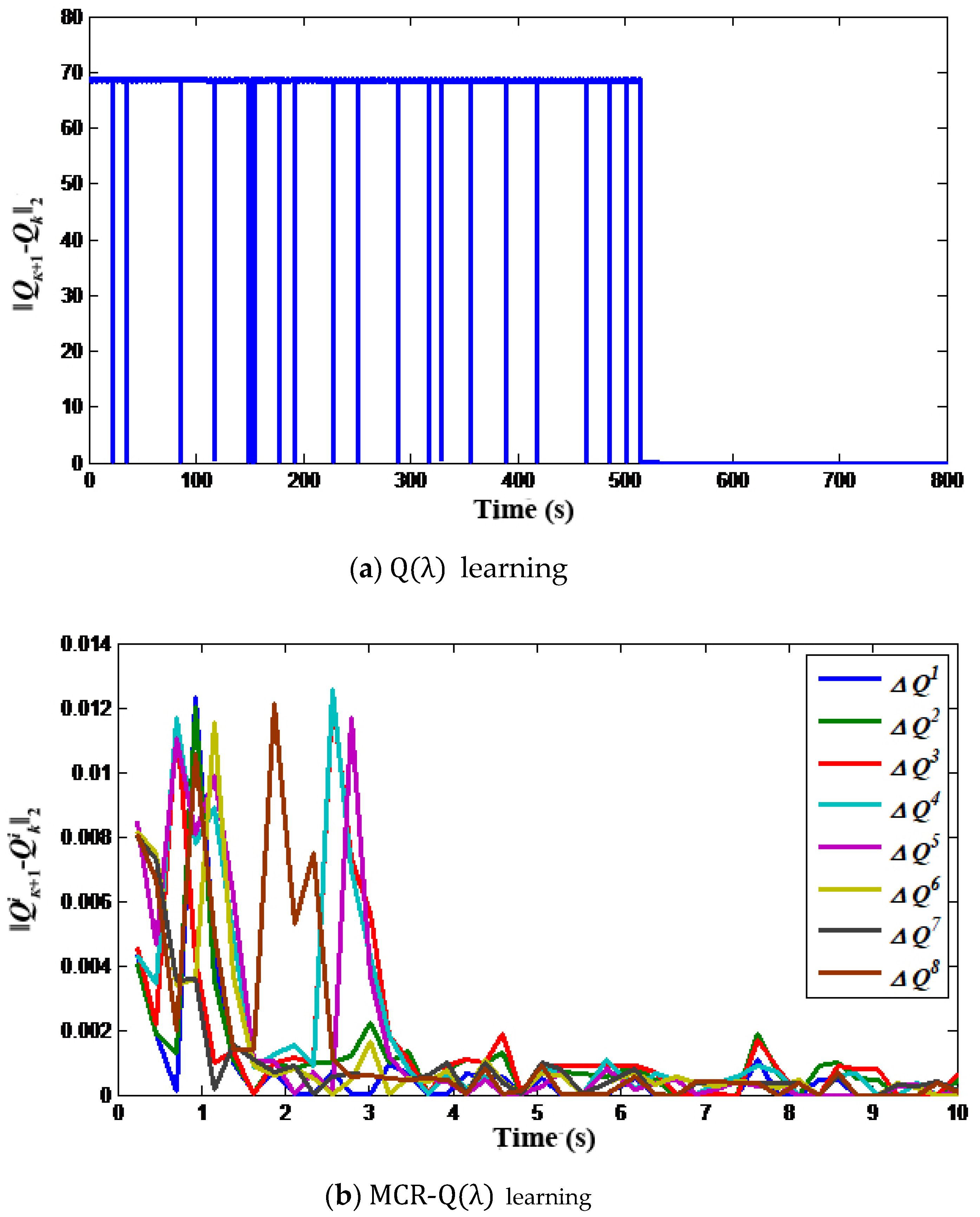
Figure 3 illustrates the convergence process of the Q-value deviation between Q(λ) learning and MCR-Q(λ) learning under scenario 1, where the Q-value deviation is defined as the 2-norm of matrix ( Q k + 1 Q k ) , that is, Q k + 1 Q k 2 . As obtained from Figure 3a, since the Q matrix of single-objective Q(λ) learning is large and the updating speed is slow, the algorithm can converge to the optimal Q* matrix through a variety of trial-and-error explorations, while the convergence time is about 530s. In contrast, after reducing the dimension of the solution space of MCR-Q(λ) learning, the Qi matrix corresponding to each variable is very small, and 20 objectives are updated at the same time. The optimization speed is more than 100 times of that of Q(λ) learning, which can converge after about 3.5 s, as shown in 
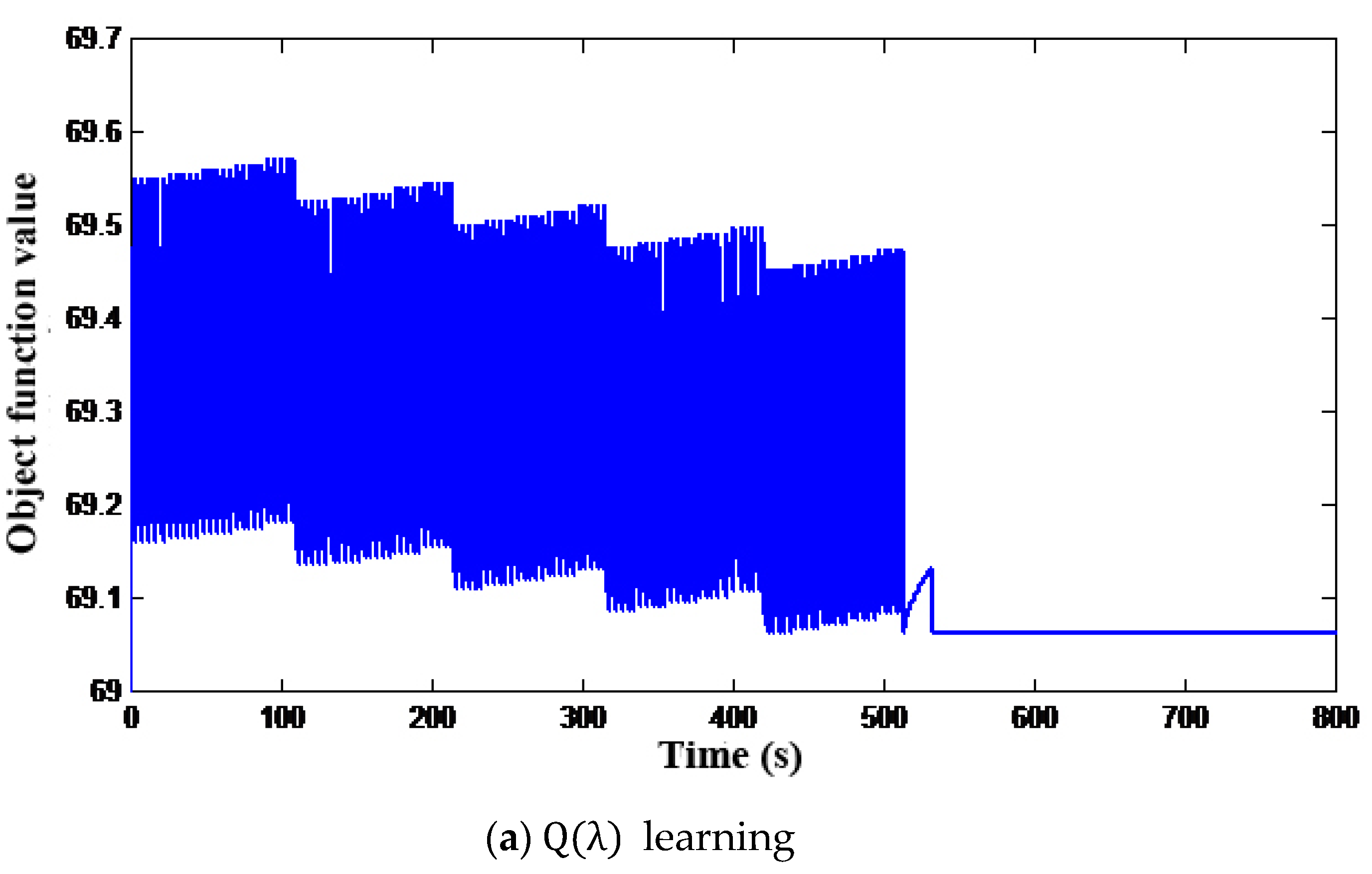
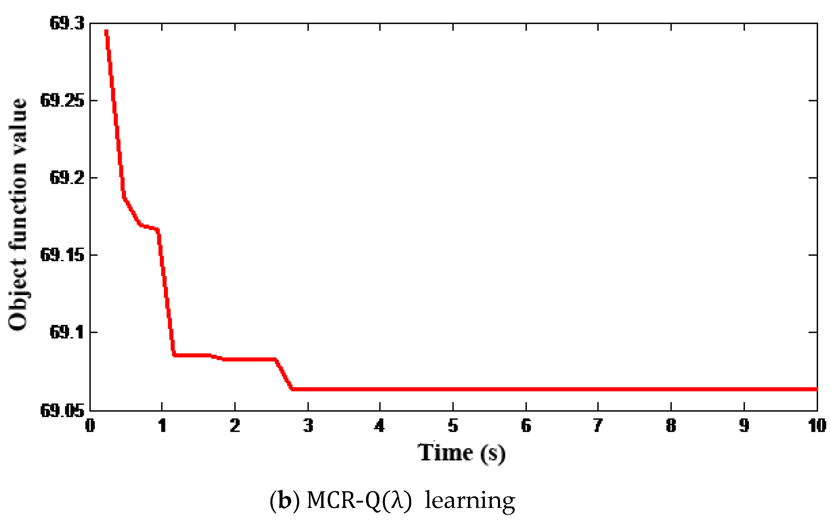
Figure 3b. Moreover, it can be obtained from the convergence of the objective function values in Figure 4 that the optimization speed of MCR-Q(λ) learning is much faster, and both algorithms can converge to the global optimal solution.
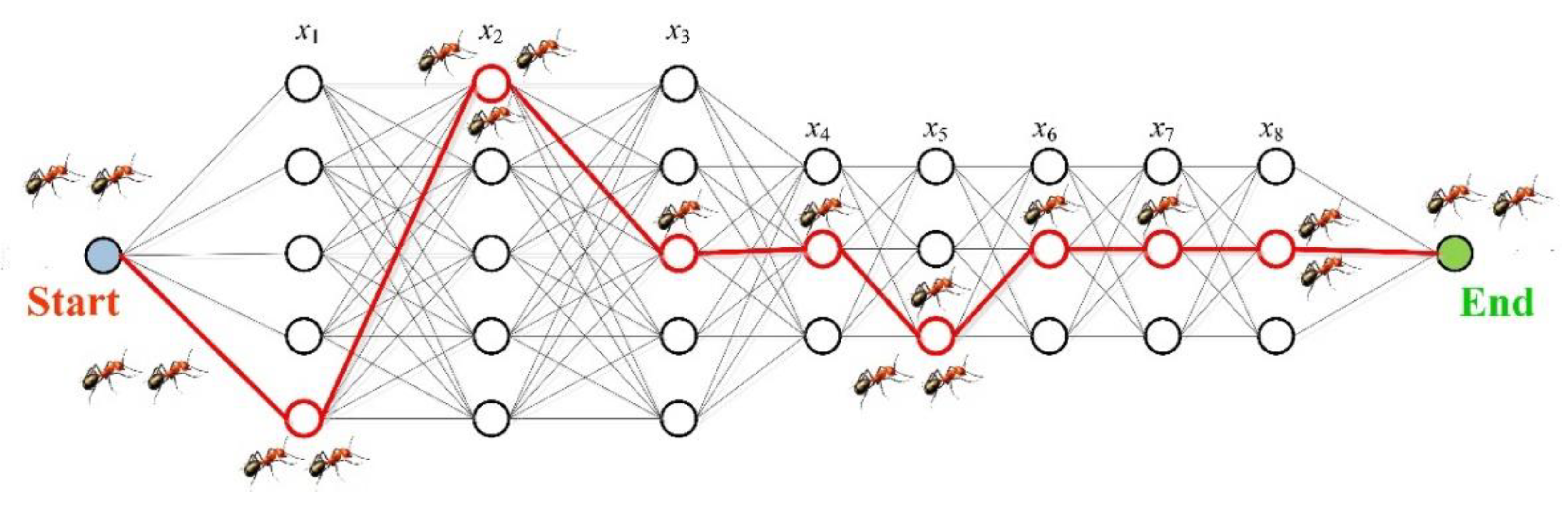
When MCR-Q(λ) learning converges, the value function matrix Qi and probability matrix Pi corresponding to all variables will prefer a state-action pair, and all individuals will tend to be consistent in selecting the action, as demonstrated in Figure 5.

6.1.3. Comparative Analysis of Simulation Results

For the purpose of evaluating the optimization capability of MCR-Q(λ) learning, this section applies all the algorithms to solve the OCECF model for 10 repetitions. For each method, the objective function value is directly taken to evaluate the quality of a solution during the searching process, which is the most crucial index to evaluate the optimization performance.
Table 5 indicates the average convergence results of 10 repetitions for the different algorithms, and it can be found that:
(a)
The optimal solution obtained by Q learning and Q(λ) learning is the best, but the optimization time is also the longest, which also shows the strong ergodicity of RL;
(b)
The convergence objective value of MCR-Q learning and MCR-Q(λ) learning is the closest to Q learning and Q(λ) learning, and the convergence time is the shortest, while the convergence speed is about 100 times that of single-objective Q learning and Q(λ) learning;
(c)
RL improves the algorithmic speed by up to 37.13% with the introduction of the eligibility trace (λ) returns mechanism;
(d)
With the increase in the load scenario, the line losses and carbon losses of the power grid will also increase correspondingly. However, since the power system has a sufficient reactive power supply, its voltage stability component just changes slightly.
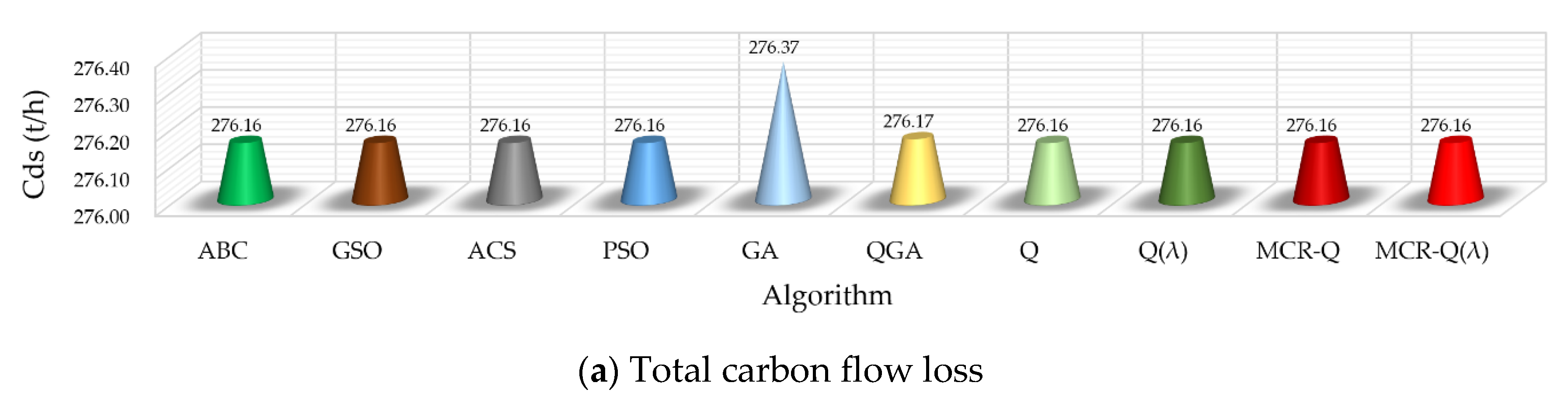
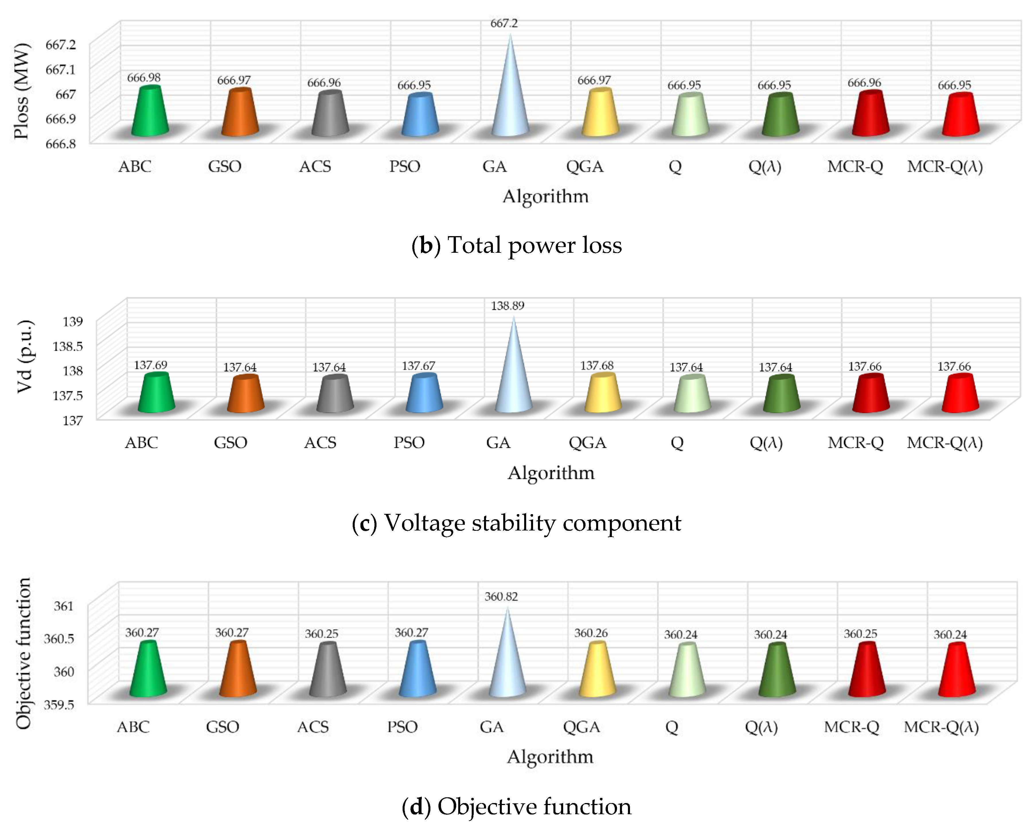
Figure 6 gives the results comparison between different methods, where each value is the average of the sum value of five scenarios in 10 runs. It is obvious that the result obtained by GA is the worst among all the methods due to its premature convergence. On the other hand, the proposed MCR-Q(λ) learning only has a slight improvement on each index compared with the other methods, but it also can obtain the lowest total carbon flow loss and objective function. It verifies that the proposed method can effectively satisfy the low-carbon requirement from the viewpoint of power networks.
Lastly, Table 6 gives the statistic convergence results of 10 repetitions for the different algorithms, and it can be found that:
(a)
The Q learning and Q(λ) learning have the highest convergence stability and can converge to the global optimal solution every time;
(b)
The statistical variance and standard deviation of MCR-Q(λ) learning are the closest to Q learning and Q(λ) learning, which have a relatively high convergence stability;
(c)
Except RL, other algorithms are more likely to trap at a local optimum because of the parameter setting and the lack of learning ability.

6.2. Case Study of the IEEE 300-Bus System

6.2.1. Simulation Model

According to different generator types, the carbon emission rate δsw of each unit in the IEEE 300-bus system is summarized in 
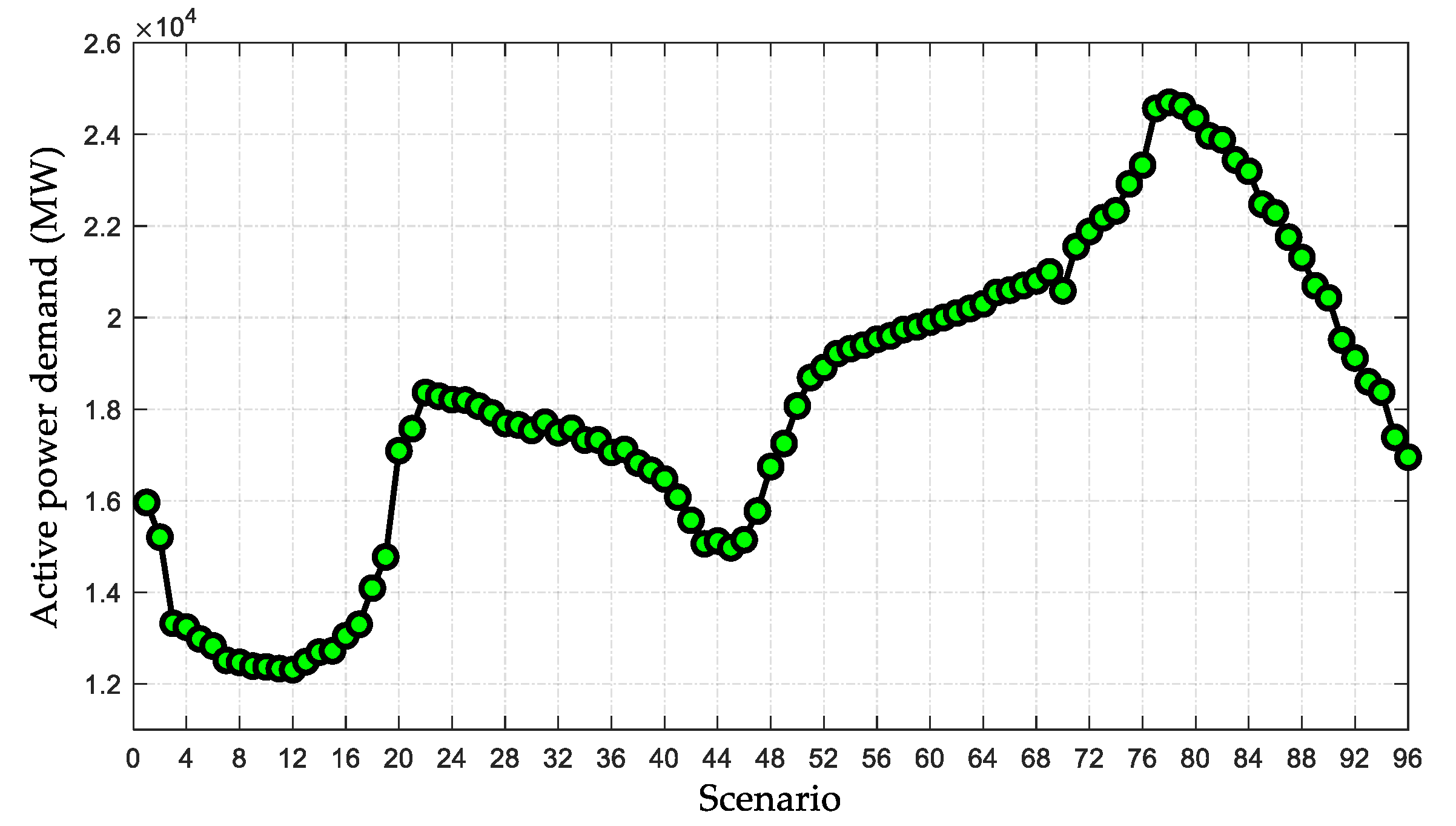
Table 7. Besides, 96 different load scenarios are designed to simulate different optimization tasks in a day for the IEEE 300-bus system, as shown in Figure 7. Moreover, the optimization variables are given in Table 8.

6.2.2. Comparative Analysis of Simulation Results

For the purpose of evaluating the optimization capability of MCR-Q(λ) learning, this section applies all the algorithms to solve the OCECF model for 10 runs. Since the number of optimization variables of the IEEE 300-bus system dramatically increases, the conventional Q and Q(λ) algorithms cannot implement an optimization due to the dimension disaster. 
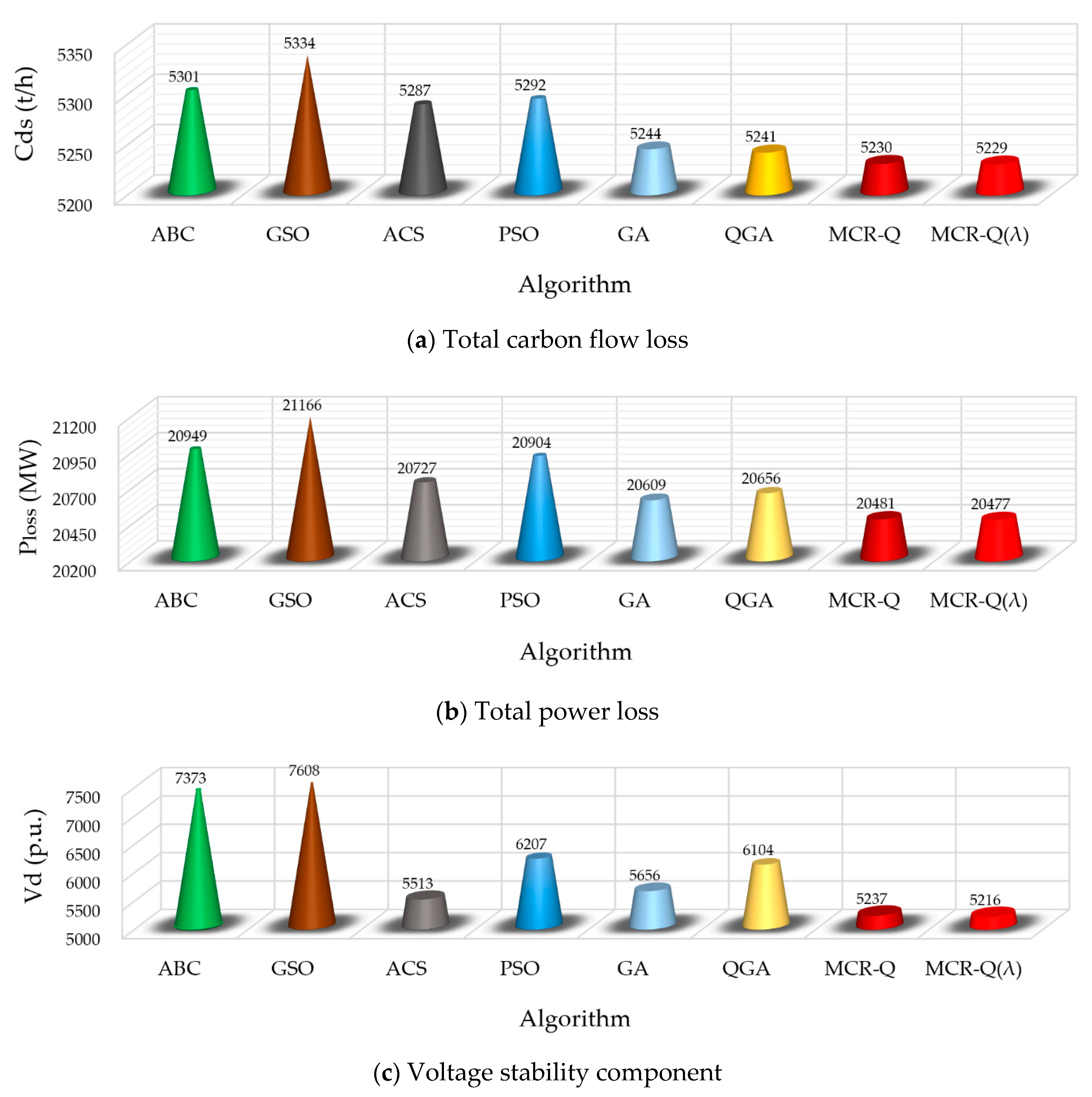
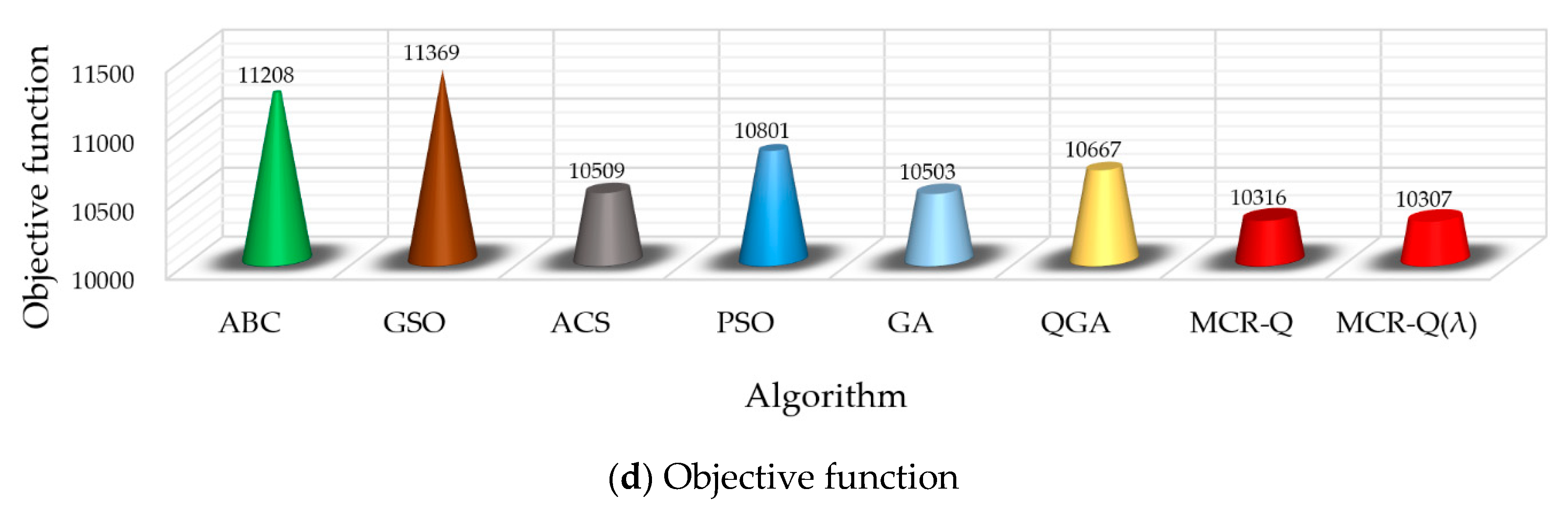
Figure 8 provides the results comparison between different methods, where each value is the average of the sum value of a day in 10 runs. It can be found that the proposed MCR-Q(λ) learning significantly outperforms other methods on the total carbon flow loss, total power loss, voltage stability component and the objective function. Hence, the MCR-Q(λ) learning-based OCECF can achieve a low-carbon operation for the power network. Particularly, these values obtained by MCR-Q(λ) learning are 2.0%, 3.4%, 45.9% and 10.3% lower than that obtained by GSO. It verifies that the optimization performance of MCR-Q(λ) is much better than other conventional meta-heuristic algorithms as the system scale increases.
Besides, Table 9 gives the distribution statistics of the objective function under different algorithms in the IEEE 300-bus system, where each value is the sum value of the objective function of a day in 10 runs; the best, worst, variance and standard deviation (Std. Dev.) are calculated to evaluate the convergence stability [51]. It can be seen from Table 9 that the convergence stability of MCR-Q(λ) learning is the highest among all the methods with the smallest variance and standard deviation of the objective function.

7. Conclusions

This paper builds an OCECF model to optimize the carbon emission and energy losses of power grids simultaneously and proposes a new MCR-Q(λ) learning to solve this problem, which has the following four contributions/novelties:
(1)
The OCECF model carefully considers the distribution of carbon flow in the power grid, which effectively resolves the carbon emission optimization at the power grid side;
(2)
MCR-Q(λ) learning is proposed for the first time, which largely reduces the dimension of the solution space, and significantly accelerates the updating rate of the Q-value matrix via multi-agent cooperative exploration learning, such that the optimization speed can be considerably accelerated;
(3)
Compared with Q(λ) learning, the convergence rate of MCR-Q(λ) learning can be increased by about 100 times, while a higher global convergence stability is guaranteed. Hence, it is very suitable for resolving dynamic OCECF in a large and complex power grid compared with other algorithms;
(4)
Like ACO, MCR-Q(λ) learning is also suitable for solving various complex optimization problems.
To further improve the operation benefit of power grids, future works can focus on the carbon trading system-based optimal power flow and the Pareto-based multi-objective learning methods, while a decentralized optimization will be studied for high operation privacy and reliability.

Author Contributions

H.C. established the model, implemented the simulation and wrote this article; C.G. guided and revised the paper and refined the language; X.H. collected references; Y.L. guided the research; T.Y. assisted in writing algorithms. All authors have read and agreed to the published version of the manuscript.

Funding

This research was funded by Technical Projects of China Southern Power Grid grant number [GDK JXM20173256].

Conflicts of Interest

The authors declare no conflict of interest.

Nomenclature

PGi, QGiactive and reactive power generation of the ith node
PDi, QDiactive and reactive power demand of the ith node
Vi, Vjvoltage magnitude of the ith and jth node
bijsusceptance of line ij
Siapparent power flow of the ith transmission line
Ninode set
NLset of branches of the power network
NGset of units
NHset of hydro units
NBset of PQ nodes
NCset of compensation equipment
NKset of on-load transformers
kton-load tap changer ratio
Qcreactive power compensation
θphase angle of each node
Vdcomponent of voltage stability
Vjmin, Vjmaxminimum and maximum voltage limit of load node j
μ1, μ2weight coefficients
Wgenerator set
(sk, ak)actual state-action pair of the kth iteration
δk, ρkestimates of Q-function errors
R(sk, sk+1, ak)reward function value of the kth iterative time environment from state sk to sk+1 through a selected action ak
aggreedy action strategy
Aaction set
LBestfunction value of an individual (i.e., the best individual) that has the least value of the target function value at the kth iteration
SABeststate-action pair set of the best individual executed at the kth iteration
γdiscount factor
λtrace-decay factor
αlearning factor
Jnumber of groups

Abbreviations

OCECFoptimal carbon-energy combined-flow
OTLCon-load tap changer
MCR-Q(λ)multi-agent cooperative reduced-dimension Q(λ)
HRLhierarchical reinforcement learning
EEDenvironmental economic dispatch

References

  1. Yang, B.; Jiang, L.; Wang, L.; Yao, W.; Wu, Q.H. Nonlinear maximum power point tracking control and modal analysis of DFIG based wind turbine. Int. J. Electr. Power Energy Syst. 2016, 74, 429–436. [Google Scholar] [CrossRef] [Green Version]
  2. Yang, Y.D.; Song, A.J.; Liu, H.; Qin, Z.J.; Deng, J.; Qi, J.J. Parallel computing of multi-contingency optimal power flow with transient stability constraints. Prot. Control Mod. Power Syst. 2018, 3, 204–213. [Google Scholar] [CrossRef] [Green Version]
  3. Yang, B.; Yu, T.; Zhang, X.S.; Li, H.F.; Shu, H.C.; Sang, Y.Y.; Jiang, L. Dynamic leader based collective intelligence for maximum power point tracking of PV systems affected by partial shading condition. Energy Convers. Manag. 2019, 179, 286–303. [Google Scholar] [CrossRef]
  4. Yang, B.; Wang, J.B.; Zhang, X.S.; Yu, T.; Yao, W.; Shu, H.C.; Zeng, F.; Sun, L.M. Comprehensive overview of meta-heuristic algorithm applications on pv cell parameter identification. Energy Convers. Manag. 2020, 208, 112595. [Google Scholar] [CrossRef]
  5. Yang, B.; Yu, T.; Shu, H.C.; Zhang, Y.M.; Chen, J.; Sang, Y.Y.; Jiang, L. Passivity-based sliding-mode control design for optimal power extraction of a PMSG based variable speed wind turbine. Renew. Energy 2018, 119, 577–589. [Google Scholar] [CrossRef]
  6. Badal, F.R.; Das, P.; Sarker, S.K.; Das, S.K. A survey on control issues in renewable energy integration and microgrid. Prot. Control Mod. Power Syst. 2019, 4, 87–113. [Google Scholar] [CrossRef] [Green Version]
  7. Li, Y.; Li, Y. Two-step many-objective optimal power flow based on knee point-driven evolutionary algorithm. Processes 2018, 6, 250. [Google Scholar] [CrossRef] [Green Version]
  8. Li, G.Y.; Li, G.D.; Zhou, M. Comprehensive evaluation model of wind power accommodation ability based on macroscopic and microscopic indicators. Prot. Control Mod. Power Syst. 2019, 4, 215–226. [Google Scholar] [CrossRef]
  9. Yang, B.; Yu, T.; Shu, H.C.; Dong, J.; Jiang, L. Robust sliding-mode control of wind energy conversion systems for optimal power extraction via nonlinear perturbation observers. Appl. Energy 2018, 210, 711–723. [Google Scholar] [CrossRef]
  10. Ji, Z.; Kang, C.; Chen, Q.; Xia, Q.; Jiang, C.; Chen, Z. Low-carbon power system dispatch incorporating carbon capture power plants. IEEE Trans. Power Syst. 2013, 28, 4615–4623. [Google Scholar] [CrossRef]
  11. Kuo, C.C.; Lee, C.Y.; Sheim, Y.C. Unit commitment with energy dispatch using a computationally effificient encoding structure. Energy Convers Manag. 2011, 52, 1575–1582. [Google Scholar] [CrossRef]
  12. Ji, B.; Yuan, X.; Li, X.; Huang, Y.; Li, W. Application of quantum-inspired binary gravitational search algorithm for thermal unit commitment with wind power integration. Energy Convers Manag. 2014, 87, 589–598. [Google Scholar] [CrossRef]
  13. Wall, T.; Stanger, R.; Santos, S. Demonstrations of coal-fired oxy-fuel technology for carbon capture and storage and issues with commercial deployment. Int. J. Greenh. Gas Control 2011, 5, S5–S15. [Google Scholar] [CrossRef]
  14. Coninck, H.D.; Benson, S.M. Carbon Dioxide capture and storage: Issues and prospects. Annu. Rev. Environ. Resour. 2014, 39, 243–270. [Google Scholar] [CrossRef]
  15. Chen, J.; Yao, W.; Zhang, C.K.; Ren, Y.; Jiang, L. Design of robust MPPT controller for grid-connected PMSG-Based wind turbine via perturbation observation based nonlinear adaptive control. Renew. Energy 2019, 134, 478–495. [Google Scholar] [CrossRef]
  16. Giras, T.C.; Talukdar, S.N. Quasi-newton method for optimal power flows. Int. J. Electr. Power Energy Syst. 1981, 3, 59–64. [Google Scholar] [CrossRef]
  17. Zhang, X.S.; Xu, Z.; Yu, T.; Yang, B.; Wang, H. Optimal mileage based AGC dispatch of a GenCo. IEEE Trans. Power Syst. 2020, 35, 2516–2526. [Google Scholar] [CrossRef]
  18. Azzam, M.; Mousa, A.A. Using genetic algorithm and TOPSIS technique for multi-objective reactive power compensation. Electr. Power Syst. Res. 2010, 80, 675–681. [Google Scholar] [CrossRef]
  19. Juan, L.I.; Yang, L.; Liu, J.L.; Yang, D.L.; Zhang, C. Multi-objective reactive power optimization based on adaptive chaos particle swarm optimization algorithm. Power Syst. Prot. Control 2011, 39, 26–31. [Google Scholar]
  20. Han, P.P.; Fan, G.J.; Sun, W.Z.; Shi, B.L.; Zhang, X.A. Research on identification of LVRT characteristics of photovoltaic inverters based on data testing and PSO algorithm. Processes 2019, 7, 250. [Google Scholar] [CrossRef] [Green Version]
  21. Yang, B.; Zhang, X.S.; Yu, T.; Shu, H.C.; Fang, Z.H. Grouped grey wolf optimizer for maximum power point tracking of doubly-fed induction generator based wind turbine. Energy Convers. Manag. 2017, 133, 427–443. [Google Scholar] [CrossRef]
  22. Yang, B.; Zhong, L.E.; Yu, T.; Li, H.F.; Zhang, X.S.; Shu, H.C.; Sang, Y.Y.; Jiang, L. Novel bio-inspired memetic salp swarm algorithm and application to MPPT for PV systems considering partial shading condition. J. Clean. Prod. 2019, 215, 1203–1222. [Google Scholar] [CrossRef]
  23. Yu, T.; Liu, J.; Chan, K.W.; Wang, J.J. Distributed multi-step Q(λ) learning for optimal power flow of large-scale power grids. Int. J. Electr. Power Energy Syst. 2012, 42, 614–620. [Google Scholar] [CrossRef]
  24. Liana, M.; Roberto, S. The Ant-Q algorithm applied to the nuclear reload problem. Ann. Nucl. Energy 2002, 29, 1455–1470. [Google Scholar]
  25. Zhao, X.-G.; Liang, L.; Meng, J.; Zhou, Y. An improved quantum particle swarm optimization algorithm for environmental economic dispatch. Expert Syst. Appl. 2020, 152, 113370. [Google Scholar]
  26. Hagh, M.T.; Kalajahi, S.M.S.; Ghorbani, N. Solution to economic emission dispatch problem including wind farms using exchange market algorithm method. Appl. Soft Comput. J. 2020, 88, 106044. [Google Scholar] [CrossRef]
  27. Ghasemi, A.; Gheydi, M.; Golkar, M.J.; Eslami, M. Modeling of wind/environment/economic dispatch in power system and solving via an online learning meta-heuristic method. Appl. Soft Comput. 2016, 43, 454–468. [Google Scholar] [CrossRef]
  28. Srivastava, A.; Das, D.K. A new Kho-Kho optimization algorithm: An application to solve combined emission economic dispatch and combined heat and power economic dispatch problem. Eng. Appl. Artif. Intell. 2020, 94, 103763. [Google Scholar] [CrossRef]
  29. He, L.; Lu, Z.; Geng, L.; Zhang, J.; Li, X.; Guo, X. Environmental economic dispatch of integrated regional energy system considering integrated demand response. Int. J. Electr. Power Energy Syst. 2020, 116, 105525. [Google Scholar] [CrossRef]
  30. Zhang, R.; Yan, K.; Li, G.; Jiang, T.; Li, X.; Chen, H. Privacy-preserving decentralized power system economic dispatch considering carbon capture power plants and carbon emission trading scheme via over-relaxed ADMM. Int. J. Electr. Power Energy Syst. 2020, 121, 106094. [Google Scholar] [CrossRef]
  31. Jin, J.; Zhou, P.; Li, C.; Guo, X.; Zhang, M. Low-carbon power dispatch with wind power based on carbon trading mechanism. Energy 2019, 170, 250–260. [Google Scholar] [CrossRef]
  32. Tan, Q.; Ding, Y.; Ye, Q.; Mei, S.; Zhang, Y.; Wei, Y. Optimization and evaluation of a dispatch model for an integrated wind-photovoltaic-thermal power system based on dynamic carbon emissions trading. Appl. Energy 2019, 253, 113598. [Google Scholar] [CrossRef]
  33. Kang, C.; Zhou, T.; Chen, Q. Carbon emission flow in network. Sci. Rep. 2012, 2, 479. [Google Scholar] [CrossRef] [PubMed]
  34. Zhou, T.; Kang, C.; Qianyao, X.U.; Chen, Q. Preliminary Investigation on a Method for carbon emission flow calculation of power system. Autom. Electr. Power Syst. 2012, 36, 44–49. [Google Scholar]
  35. Li, B.; Song, Y.; Hu, Z. Carbon flow tracing method for assessment of demand side carbon emissions obligation. IEEE Trans. Sustain. Energy 2013, 4, 1100–1107. [Google Scholar] [CrossRef]
  36. Zhang, X.S.; Yu, T.; Yang, B.; Zheng, L.M.; Huang, L.N. Approximate ideal multi-objective solution Q(λ) learning for optimal carbon-energy combined-flow in multi-energy power systems. Energy Convers. Manag. 2015, 106, 543–556. [Google Scholar] [CrossRef]
  37. Zhang, X.; Tan, T.; Zhou, B.; Yu, T.; Yang, B.; Huang, X. Adaptive distributed auction-based algorithm for optimal mileage based AGC dispatch with high participation of renewable energy. Int. J. Electr. Power Energy Syst. 2021, 124, 106371. [Google Scholar] [CrossRef]
  38. Sutton, R.S. Learning to predict by the methods of temporal differences. Mach. Learn. 1988, 3, 9–44. [Google Scholar] [CrossRef]
  39. Tao, Y.U.; Wang, Y.M.; Zhen, W.G.; Wenjia, Y.E.; Liu, Q.J. Multi-step backtrack Q-learning based dynamic optimal algorithm for auto generation control order dispatch. Control Theory Appl. 2011, 28, 58–64. [Google Scholar]
  40. Ghavamzadeh, M.; Mahadevan, S. Hierarchical average reward reinforcement learning. J. Mach. Learn. Res. 2017, 8, 2629–2669. [Google Scholar]
  41. Cao, H.Z.; Yu, T.; Zhang, X.S.; Yang, B.; Wu, Y.X. Reactive power optimization of large-scale power system: A transfer bees optimizer application. Processes 2019, 7, 321. [Google Scholar] [CrossRef] [Green Version]
  42. Xiong, Y.; Chen, H.H.; Miao, F.Y.; Wang, X.F. A quantum genetic algorithm to solve combinatorial optimization problem. Acta Electron. Sin. 2004, 32, 1855–1858. [Google Scholar]
  43. Kumari, M.S.; Maheswarapu, S. Enhanced genetic algorithm based computation technique for multi-objective optimal power flow solution. Int. J. Electr. Power Energy Syst. 2010, 32, 736–742. [Google Scholar] [CrossRef]
  44. Hazra, J.; Sinha, A.K. A multi-objective optimal power flow using particle swarm optimization. Eur. Trans. Electr. Power 2011, 21, 1028–1045. [Google Scholar] [CrossRef]
  45. Han, Y.; Shi, P. An improved ant colony algorithm for fuzzy clustering in image segmentation. Neurocomputing 2007, 70, 665–671. [Google Scholar] [CrossRef]
  46. Basu, M. Group search optimization for solution of different optimal power flow problems. Electr. Mach. Power Syst. 2016, 44, 10. [Google Scholar] [CrossRef]
  47. Karaboga, D.; Basturk, B. On the performance of artificial bee colony (ABC) algorithm. Appl. Soft Comput. 2008, 8, 687–697. [Google Scholar] [CrossRef]
  48. Zimmerman, R.D.; Murillo-Sánchez, C.E.; Thomas, R.J. Matpower: Steady-state operations, planning and analysis tool for power systems research and education. IEEE Trans. Power Syst. 2011, 26, 12–19. [Google Scholar] [CrossRef] [Green Version]
  49. MATPOWER—Free, Open-Source Tools for Electric Power System Simulation and Optimization. Available online: https://matpower.org/ (accessed on 21 May 2020).
  50. Mahmoud, K.; Abdel-Nasser, M.; Mustafa, E.; Ali, Z.M. Improved salp-swarm optimizer and accurate forecasting model for dynamic economic dispatch in sustainable power systems. Sustainability 2020, 12, 576. [Google Scholar] [CrossRef] [Green Version]
  51. Zhang, X.S.; Yu, T.; Yang, B.; Cheng, L.F. Accelerating bio-inspired optimizer with transfer reinforcement learning for reactive power optimization. Knowl. Based Syst. 2017, 116, 26–38. [Google Scholar] [CrossRef]
Figure 1. The carbon-energy combined-flow (CECF) structure in power systems.
Energies 13 04778 g001
Figure 2. Difference between Q(λ) and MCR-Q(λ).
Energies 13 04778 g002
Figure 3. Q-value difference convergence.
Energies 13 04778 g003
Figure 4. Convergence process of the objective function value.
Energies 13 04778 g004aEnergies 13 04778 g004b
Figure 5. Convergent results of state-action pairs by MCR-Q(λ) learning.
Energies 13 04778 g005
Figure 6. Comparison of results obtained by different methods in the IEEE 118-bus system.
Energies 13 04778 g006aEnergies 13 04778 g006b
Figure 7. The load scenarios of the IEEE 300-bus system.
Energies 13 04778 g007
Figure 8. Comparison of results obtained by different methods in the IEEE 300-bus system.
Energies 13 04778 g008aEnergies 13 04778 g008b
Table 1. Parameter setting of MCR-Q(λ) learning.
ParametersRangeValue
γ0 < γ < 10.1
λ0 < λ < 10.5
α0 < α < 10.1
q00 < q0 < 10.8
JJ > 120
WW > 01
Table 2. Carbon emission rate of the IEEE 118-bus system.
Generator NodeGenerator Typeδsw (kg/kW·h)Generator NodeGenerator Typeδsw (kg/kW·h)
1Gas0.565Hydro0
4Hydro066Wind0
6Coal1.0669Gas0.5
8Coal1.0170Hydro0
10Coal0.9572Coal1.06
12Coal1.573Coal1.01
15Coal0.774Coal0.95
18Gas0.576Coal1.5
19Hydro077Coal0.7
24Hydro080Hydro0
25Coal1.0185Hydro0
26Coal0.9587Gas0
27Coal1.589Wind0
31Wind090Gas1.01
32Coal1.0691Coal0.95
34Coal1.0192Coal1.5
36Coal0.9599Coal0
40Coal1.5100Hydro0
42Coal0.7103Hydro0
46Hydro0104Gas1.06
49Hydro0105Coal1.01
54Gas0.5107Coal0.95
55Photovoltaic0110Coal1.5
56Coal1.01111Coal0.7
59Coal0.95112Coal0
61Coal1.5113Hydro0
62Hydro0116Hydro0
Table 3. Load statistical conditions employed in five scenarios.
ScenariosActive Power (MW)
Node 54Node 59Node 80Node 90Node 116
191221105131148
2102249118147166
3113277131163184
4124305144179202
5135333157192220
Table 4. Optimization variables of the IEEE 118-bus system.
Variable TypeNumber of BusAction SpaceVariable Number
Reactive power compensation45, 79, 105{−40%, −20%, 0%, 20%, 40%}3
OLTC ratio8–5, 26–25, 30–17, 63–59, 64–61{0.98, 1.00, 1.02}5
Table 5. Average results of different algorithms on the IEEE 118-bus system in 10 runs.
ScenariosIndexesABCGSOACSPSOGAQGAQQ(λ)MCR-QMCR-Q(λ)
1Time (s)55.0813.30 13.68 31.44 17.14 20.53 660.00 608.00 5.75 5.27
Cds (t/h)50.7150.71 50.71 50.71 50.77 50.71 50.71 50.71 50.71 50.71
Ploss (MW)128.85128.85 128.85 128.85 128.91 128.85 128.85 128.85 128.85 128.85
Vd27.6527.63 27.63 27.64 27.86 27.65 27.63 27.63 27.63 27.64
Objective69.0769.07 69.06 69.07 69.18 69.07 69.06 69.06 69.06 69.06
2Time (s)65.7315.83 8.93 29.72 16.44 16.52 646.00 450.00 4.14 3.43
Cds (t/h)52.6952.69 52.69 52.69 52.73 52.70 52.69 52.69 52.69 52.69
Ploss (MW)130.24130.23 130.23 130.23 130.28 130.24 130.23 130.23 130.23 130.23
Vd27.5827.56 27.56 27.57 27.70 27.58 27.56 27.56 27.57 27.57
Objective70.1770.16 70.16 70.17 70.23 70.17 70.16 70.16 70.17 70.16
3Time (s)36.7512.66 23.69 49.40 15.57 12.35 671.00 445.00 4.92 3.09
Cds (t/h)54.9254.92 54.92 54.92 54.95 54.92 54.92 54.92 54.92 54.92
Ploss (MW)132.50132.50 132.49 132.49 132.53 132.49 132.49 132.49 132.49 132.49
Vd27.5227.52 27.52 27.53 27.74 27.52 27.52 27.52 27.53 27.52
Objective71.6571.65 71.64 71.65 71.74 71.64 71.64 71.64 71.64 71.64
4Time (s)44.1116.65 10.16 52.77 15.93 14.33 663.00 447.00 4.70 4.30
Cds (t/h)57.4857.48 57.48 57.48 57.52 57.48 57.48 57.48 57.48 57.48
Ploss (MW)135.66135.66 135.66 135.66 135.72 135.66 135.66 135.66 135.66 135.66
Vd27.4927.48 27.48 27.48 27.85 27.48 27.48 27.48 27.48 27.48
Objective73.5473.54 73.54 73.54 73.70 73.54 73.54 73.54 73.54 73.54
5Time (s)26.4318.41 7.67 42.65 14.27 12.92 658.00 441.00 6.37 5.01
Cds (t/h)60.3660.36 60.36 60.36 60.40 60.36 60.36 60.36 60.36 60.36
Ploss (MW)139.73139.73 139.73 139.72 139.76 139.73 139.72 139.72 139.73 139.72
Vd27.4527.45 27.45 27.45 27.74 27.45 27.45 27.45 27.45 27.45
Objective75.8475.85 75.85 75.84 75.97 75.84 75.84 75.84 75.84 75.84
Table 6. Distribution statistics of the objective function under different algorithms in the IEEE 118-bus system in 10 runs.
ScenariosCriteriaABCGSOACSPSOGAQGAQQ(λ)MCR-QMCR-Q(λ)
1Best69.0669.0669.0669.0669.0669.0669.0669.0669.0669.06
Worst69.0969.0869.0769.0969.3669.1169.0669.0669.0669.07
Variance1.2 × 10−42.7 × 10−55.9 × 10−65.5 × 10−58.4 × 10−32.2 × 10−40001.6 × 10−6
Standard deviation1.1 × 10−25.2 × 10−32.4 × 10−37.4 × 10−39.1 × 10−21.5 × 10−20001.3 × 10−3
2Best70.1670.1670.1670.1670.1670.1670.1670.1670.1670.16
Worst70.2270.1770.1670.1970.3370.2070.1670.1670.2070.17
Variance3.0 × 10−45.7 × 10−605.5 × 10−54.1 × 10−32.3 × 10−4001.5 × 10−42.8 × 10⁻⁶
Standard deviation1.7 × 10−22.4 × 10−307.4 × 10−36.4 × 10−21.5 × 10−2001.2 × 10−21.7 × 10⁻³
3Best71.6471.6471.64 71.6471.6471.64 71.6471.6471.6471.64
Worst71.6671.6571.66 71.6971.9671.65 71.6471.6471.6571.64
Variance2.4 × 10−51.3 × 10−52.3 × 10−52.7 × 10−41.0 × 10−25.6 × 10−6008.2 × 10−60
Standard deviation5.3 × 10−33.6 × 10−34.8 × 10−31.6 × 10−21.0 × 10−12.4 × 10−3002.9 × 10−30
4Best73.5473.5473.5473.5473.5473.5473.5473.5473.5473.54
Worst73.5773.5573.5573.5473.8773.5473.5473.5473.5473.54
Variance7.6 × 10−55.7 × 10−62.3 × 10−501.0 × 10−200000
Standard deviation8.7 × 10−32.4 × 10−34.8 × 10−301.0 × 10−100000
5Best75.8475.8475.8475.8475.8475.8475.8475.8475.8475.84
Worst75.8575.8575.8675.8476.1275.8575.8475.8475.8575.84
Variance5.7 × 10−61.3 × 10−52.6 × 10−508.7 × 10−31.6 × 10−6005.7 × 10−60
Standard deviation2.4 × 10−33.6 × 10−35.1 × 10−309.3 × 10−21.3 × 10−3002.4 × 10−30
Table 7. Carbon emission rate of the IEEE 300-bus system.
Generator NodeGenerator Typeδsw (kg/kWh)Generator NodeGenerator Typeδsw (kg/kWh)Generator NodeGenerator Typeδsw (kg/kWh)
8Hydro0171Hydro07002Hydro0
10Photovoltaics0176Hydro07003Coal1.06
20Coal1.01177Hydro07011Coal1.5
63Coal0.95185Coal1.017012Coal0.7
76Coal1.5186Coal0.957017Photovoltaics0
84Coal0.7187Coal1.57023Gas0.5
91Coal0.95190Hydro07024Hydro0
92Coal1.5191Hydro07039Wind0
98Coal0.7198Hydro07044Coal1.5
108Hydro0213Hydro07049Coal0.7
119Gas0.5220Wind07055Hydro0
124Coal1.06221Gas0.57057Wind0
125Coal1.01222Coal1.067061Coal1.06
138Hydro0227Coal1.017062Coal1.01
141Hydro0230Coal0.957071Coal1.01
143Coal1.06233Coal1.57130Hydro0
146Coal1.01236Coal0.77139Hydro0
147Coal0.95238Coal0.957166Coal0.7
149Coal1.5239Hydro09002Gas0.5
152Hydro0241Hydro09051Coal1.06
153Photovoltaics0242Coal0.959053Coal1.01
156Coal1.06243Coal1.59054Hydro0
170Coal0.957001Coal0.959055Photovoltaics0
Table 8. Optimization variables of the IEEE 300-bus system.
Variable TypeNumber of BusAction SpaceVariable Number
Reactive power compensation117, 120, 154, 164, 166, 173, 190, 231, 238, 240, 248{−40%, −20%, 0%, 20%, 40%}11
OLTC ratio9021–9022, 9002–9024, 9023–9025, 9023–9026, 9007–9071, 9007–9072, 9003–9031, 9003–9032, 9003–9033, 9004–9041, 9004–9042, 9004–9043, 9003–9034, 9003–9035, 9003–9036, 9003–9037, 9003–9038, 213–214, 222–237, 227–231, 241–237, 45–46, 73–74, 81–88, 85–99, 86–102, 122–157, 142–175, 145–180, 200–248, 211–212, 223–224, 196–2040, 7003–3, 7003–61, 7166–166, 7024–24, 7001–1, 7130–130, 7011–11, 7023–23, 7049–49, 7139–139, 7012–12{0.98, 1.00, 1.02}44
Table 9. Distribution statistics of the objective function under different algorithms in the IEEE 300-bus system in 10 runs.
CriteriaABCGSOACSPSOGAQGAMCR-QMCR-Q(λ)
Best11,182.9711,328.3810,505.5810,795.7310,495.0310,658.2810,312.8410,305.54
Worst11,229.6111,404.3510,513.4010,812.5410,509.0310,675.3410,320.8610,308.30
Variance246.73541.7910.2545.6223.9632.5710.121.20
Standard deviation15.7123.283.206.754.895.713.181.09

