Dynamic Electro-Thermal PV Temperature and Power Output Prediction Model for Any PV Geometries in Free-Standing and BIPV Systems Operating under Any Environmental Conditions

Abstract

PV temperature significantly affects the module’s power output and final system yield, and its accurate prediction can serve the forecasting of PV power output, smart grid operations, online PV diagnostics and dynamic predictive management of Building Integrated Photovoltaic (BIPV) systems. This paper presents a dynamic PV temperature prediction model based on transient Energy Balance Equations, incorporating theoretical expressions for all heat transfer processes, natural convection, forced convection, conduction and radiation exchanges between both module sides and the environment. The algorithmic approach predicts PV temperature at the centre of the cell, the back and the front glass cover with fast convergence and serves the PV power output prediction. The simulation model is robust, predicting PV temperature with high accuracy at any environmental conditions, PV inclination, orientation, wind speed and direction, and mounting configurations, free-standing and BIPV. These, alongside its theoretical basis, ensure the model’s wide applicability and clear advantage over existing PV temperature prediction models. The model is validated for a wide range of environmental conditions, PV geometries and mounting configurations with experimental data from a sun-tracking, a fixed angle PV and a BIPV system. The deviation between predicted and measured power output for the fixed-angle and the sun-tracking PV systems was estimated at −1.4% and 1.9%, respectively. The median of the temperature difference between predicted and measured values was as low as 0.5 °C for the sun-tracking system, and for all cases, the predicted temperature profiles were closely matching the measured profiles. The PV temperature and power output predicted by this model are compared to the results produced by other well-known PV temperature models, illustrating its high predictive capacity, accuracy and robustness.

1. Introduction

The modelling of photovoltaic (PV) temperature has received increased attention in recent years in an effort to accurately predict the power output and final yield of PV systems. The increase in PV temperature during PV operation leads to a significant reduction in module power output and operating efficiency, with the temperature coefficient for the maximum power P_m of a typical value −0.5%/°C for c-Si PV modules [1,2]. This translates to a reduction in PV power output from the rated peak power in the range of 5–25%, due to PV temperature alone, considering 1000 W/m² solar irradiance incident on the PV plane. The effect is in the higher end of this range for Building Integrated Photovoltaic (BIPV) systems [3]. This has led to the need for accurate PV temperature prediction models to serve the forecasting of PV power output and smart grid operations, optimum PV system sizing, online PV diagnostics and the dynamic predictive management of BIPV in Intelligent Energy Buildings.

Several empirical and semi-empirical PV temperature models have been proposed in the research literature, mainly taking into account the solar irradiance on the PV plane I_T, the ambient temperature T_α, and the wind speed v_w. These include the well-known models by King et al. [4], Faiman [5], and others, as reviewed in [6,7,8].

King et al. [4] have proposed the exponential form of Equation (1) for the estimation of PV temperature at the back of the module T_PVb and the temperature of the cell at the centre T_PVc given by Equation (2), for both free-standing and insulated back modules

$$T_{PVb}=T_a+I_T·e^{\left(a+b·v_w\right)}$$

(1)

$$T_{PVc}=T_{PVb}+\mathsf{\Delta }{\rm T}·{{\rm I}}_{{\rm T}}/1000$$

(2)

where coefficients α, b were empirically determined and were defined along with the temperature difference ΔΤ between the centre of the cell and the back of the module, according to the following [4]:

a = −3.56, b = −0.0750, ΔΤ = 3 °C for glass/cell/polymer sheet, open rack module;

a = −2.81, b = −0.0455, ΔΤ = 0 °C for glass/cell/polymer sheet, insulated back module.

Faiman has proposed the following model [5]

$$T_{pv}=T_a+I_T/\left(U_o^{\prime }+U_1^{\prime }·v_w\right)$$

(3)

where $U_o^{\prime }, U_1^{\prime }$ are empirically determined coefficients with average values: $U_o^{\prime }=25 \mathrm{W}{\mathrm{m}}^{-2}{\mathrm{K}}^{-1}$ and $U_1^{\prime }=6.84 \mathrm{W}{\mathrm{m}}^{-3}\mathrm{s}{\mathrm{K}}^{-1}$.

PV module technology, structure and mounting configurations have been considered in the above models through the empirically determined coefficients, while validation of these models’ applicability at different climatic regions is presented in [9].

NN-based models have been proposed, such as the model by Tamizhmani et al. [10], independent of site location and technology type, and expressed through Equation (4).

$$T_{pv}=0.943T_a+0.028I_T-1.528v_w+4.3$$

(4)

Multiple regression analysis and numerical approaches have also been proposed with promising results [11,12]. Several theoretical models based on the Energy Balance Equation (EBE), both steady-state and transient have been developed, such as [13,14,15,16,17,18,19,20]. However, these make use of empirical models for the determination of the air-forced convection coefficient or other simplifications and assumptions, while the geometry of the PV modules with respect to the wind direction is neglected or only considered through existing empirical expressions for the windward or leeward side. These limit the models’ applicability to the experimental setup and conditions, based on which these empirical expressions were derived. It was previously shown by the authors [21] that the air-forced convection coefficient has a significant effect on the T_pv prediction, highlighting the importance of theoretical models over empirical ones for the determination of the air-forced convection coefficient. The simulation model developed in [21] determines the f coefficient in Equation (5) based on theoretical expressions for the heat convection coefficients, with a separate approach to the windward and leeward side of the module, at any PV inclination, orientation and wind direction. It determines the natural convection at any PV inclination angle for the front and back side of the PV module, and the radiation exchanges between the module, front and back PV side, and the environment. Therefore, the f coefficient incorporates all these effects

$$T_{pv}=T_a+f·I_T$$

(5)

$$f=\frac{\left(\tau \alpha \right)-{\eta }_{pv}}{U_{L,f}+U_{L,b}}$$

(6)

where (τα) is the transmittance-absorptance product and η_pv the operating PV efficiency. U_L,f and U_L,b are the thermal losses coefficients for the front and back PV side, respectively, including both convective and radiative heat transfer processes, as analyzed in Section 2. The aforementioned analysis for the heat transfer and radiative heat processes was incorporated in [22] within a steady state model and proved to provide promising results for the prediction of PV temperature at any mounting configurations and steady state conditions.

The literature review in PV temperature and power output prediction discloses the need for a model satisfying all the following requirements:

• To be theoretically robust, complete, and reliable;
• To be based on a full set of expressions to accurately describe all the electro-thermal processes within the module, and between the module and the environment;
• To respond to varying environmental conditions (ambient temperature, solar irradiance, wind speed, wind direction), incorporating transient effects
• To be applicable to any PV geometry (inclination, orientation) and mounting configuration (free-standing, BAPV, BIPV);
• To be accurate and validated with experimental data across a wide range of conditions.

In this paper, a dynamic PV temperature and power output prediction model is developed and validated, fully addressing all the aforementioned issues answering this gap in the literature view. The model is based on a set of Energy Balance Equations of transient form incorporating theoretical expressions for all heat transfer processes within the cell and towards the environment, including natural convection, forced convection, conduction and radiation exchanges between both module sides and the environment. The algorithmic approach predicts PV temperature at the centre of the cell, the back and the front glass cover with fast convergence and serves the PV power output prediction. The simulation model is robust, predicting PV temperature with high accuracy at any environmental conditions, PV inclination, orientation, wind speed and direction, and mounting configurations, free-standing and BIPV. These alongside its theoretical basis ensure the model’s wide applicability and clear advantage over existing PV temperature prediction models. The model is validated with the experimental data of over a year, covering a wide range of environmental conditions, PV geometries and mounting configurations from a sun-tracking, a fixed angle PV, and a BIPV system, while it is further compared to the results produced by the aforementioned PV temperature models [4,5,10], illustrating its high predictive capacity, accuracy and robustness.

This model applies to in-land systems, and therefore limitations may be identified with regards to PV operating in fresh water or sea environments, Floating PV (FPV) systems, or water content in the air, as well as cases of Concentrating PV (CPV) systems, or PV thermal (PV/T), but it may be adapted to additionally address these cases in the future. It is developed for conventional c-Si PV module technology glass-to-Tedlar, but may be easily adapted through the material properties to cover glass-to-glass or other module and PV technologies.

2. Transient PV Temperature and Power Output Prediction Model

The energy balance equation for transient conditions considers (1) the incident solar irradiance converted into electrical power within the cell with operating efficiency η_c, (2) the resistance to heat conduction from the cell to the glass R_c−f and to the back surface R_c−b including that of EVA, (3) the heat transfer through natural and forced convection from the front and the back PV module side, through U_L,f and U_L,b, respectively; the latter include the radiative heat exchanges between the module sides and the environment—sky and ground—and (4) the thermal energy stored in the layers of the module, and is described by the following equations.

$${\left(m{c}_p\right)}_{total}\frac{d{T}_{PVc}}{dt}=\left(\left(\tau \alpha \right)-{\eta }_c\right)I_T-\left(T_{PVc}-T_a\right)\left(\frac{1}{R_{c-f}+\frac{1}{U_{L,f}}}+\frac{1}{R_{c-b}+\frac{1}{U_{L,b}}}\right)$$

(7)

$$({\left(m{c}_p\right)}_{glass}+{\left(m{c}_p\right)}_{EVA})\frac{d{T}_{PVf}}{dt}=\left(T_{PVc}-T_{PVf}\right)\left(\frac{1}{R_{c-f}}\right)-\left(T_{PVf}-T_a\right)U_{L,f}$$

(8)

$$({\left(m{c}_p\right)}_{tedlar}+{\left(m{c}_p\right)}_{EVA})\frac{d{T}_{PVb}}{dt}=\left(T_{PVc}-T_{PVb}\right)\left(\frac{1}{R_{c-b}}\right)-\left(T_{PVb}-T_a\right)U_{L,b}$$

(9)

The mass heat capacity (mc_p) for the various layers of the module is expressed in the above equations normalised to the unit surface, with value for the front glass 4500 JK⁻¹m⁻², the EVA 502 JK⁻¹m⁻², the c-Si solar cell 355 JK⁻¹m⁻², and the Tedlar 150 JK⁻¹m⁻², [23]. (mc_p)_total = Σ(mc_p)_i, where i refers to each of the above layers. The material properties and geometry of the different layers are provided in [23].

For sun-tracking PV systems (τα) is considered equal to the transmittance-absorptance product at normal incidence (τα)_n; a typical value in this case is 0.86. For a fixed angle PV system or BIPV system, the (τα) product is strongly affected by the angle of incidence of solar irradiance on the PV plane throughout the day and is determined through Equation (10) considering the beam, diffuse and ground-reflected irradiance components, [24].

$$\frac{\left(\tau \alpha \right)}{{\left(\tau \alpha \right)}_n}=\frac{I_b{R}_b\frac{{\left(\tau \alpha \right)}_b}{{\left(\tau \alpha \right)}_n}+I_d\frac{{\left(\tau \alpha \right)}_d}{{\left(\tau \alpha \right)}_n}\frac{\left(1+cos\beta \right)}{2}+rI\frac{{\left(\tau \alpha \right)}_r}{{\left(\tau \alpha \right)}_n}\frac{\left(1-cos\beta \right)}{2}}{I_T}$$

(10)

The ratio of the transmittance-absorptance product at a certain angle of incidence to the transmittance-absorptance product at normal incidence, is known as the incidence angle modifier (IAM) or K_τα. Here, K_τα for each of the three components, beam, diffuse and ground-reflected, (τα)_b/(τα)_n, (τα)_d/(τα)_n and (τα)_r/(τα)_n respectively, is estimated based on Equation (11), with b_o = 0.136 using for the beam component the incidence angle θ, and for the diffuse and ground-reflected components the effective angle of incidence of the diffuse radiation θ_d and the effective angle of incidence of the ground-reflected radiation θ_r respectively, according to well-known expressions provided in [24].

$$K_{\tau \alpha }=1-b_o\left(\frac{1}{cos\theta }-1\right)$$

(11)

The thermal losses coefficients for the front and back PV side are given by

$$U_{L,f}=h_{c,g-a}+h_{r,g-a}$$

(12a)

$$U_{L,b}=h_{c,b-a}+h_{r,b-a}$$

(12b)

where h_c,g−a and h_c,b−a the overall heat convection coefficient from the module glass and the module back surface to the environment considering natural and forced convection. For the determination of the overall value of h, the Grashof number, Reynolds number and ratio Gr_L/Re_L² are estimated as defined in [25] and, specifically, in case (a) Gr_L << Re_L² the natural convection is neglected, (b) Gr_L >> Re_L² the forced convection is neglected, (c) 0.01 < Gr_L/Re_L² < 100 combined natural and forced convection is considered. The combined natural and forced flow is estimated through Churchill’s expressions, with m = 3 [26]

$$h_{c,g-a}^m=h_{c,g-a \left(natural\right)}^m+h_{c,g-a \left(forced\right)}^m$$

(13a)

$$h_{c,b-a}^m=h_{c,b-a \left(natural\right)}^m\pm h_{c,b-a \left(forced\right)}^m$$

(13b)

The natural heat convection coefficient from PV glass to the environment h_{c,g−a (natural)} and PV back surface to the environment h_{c,b−a (natural)} is determined through the Nu number from the general expression: $Nu=h·L/k_a$, where L is the length of the module along the natural air flow direction and k_a is the thermal conductivity of air at the boundary layer temperature. All fluid properties are calculated at the boundary layer temperature for the front and back PV module side accordingly. The boundary layer temperature T_bl for each of the sides is estimated according to the predicted PV temperature at the respective PV side, based on the expression T_bl = T_PV − 0.25∙(T_PV − T_a). This is updated in each iterative process, as described further below. The Nu number is estimated for the front PV side Nu_f, considering a hot surface facing upward and the back PV side Nu_b, considering a hot surface facing downward according to the expressions analysed by the authors in [21] for the entire range of PV inclination angles.

The simulation model takes into consideration the wind velocity and its direction, the PV module orientation and inclination, and determines the windward and leeward side of the PV module whether front or back, for the determination of the air-forced heat convection coefficient h. The latter for the windward side of the module is estimated based on the Sartori’s expressions according to the air flow whether laminar, fully turbulent or mixed, Equation (14a–c), [27]. These were shown to lead to very accurate predictions of the f coefficient [21]. This includes the decay of the heat transfer along the length of the surface in the wind direction L. The type of flow is evaluated based on the ratio x_c/L ≥ 0.95, x_c/L ≤ 0.05 and x_c/L < 0.95 for the laminar, fully turbulent and mixed flows respectively, where x_c is the critical length based on the critical Reynolds number Re_x,c.

$$h=3.83·v_w^{0.5}·L^{-0.5}for laminar flow$$

(14a)

$$h=5.74·v_w^{0.8}·L^{-0.2} for fully turbulent flow$$

(14b)

$$h=5.74·v_w^{0.8}·L^{-0.2}-16.46·L^{-1} for mixed flows$$

(14c)

For the leeward side of the PV module, the above expressions were used in the model but with L given by 4A/S, where A the area of the module and S its perimeter [21].

The thermal radiation coefficients h_r,g−a and h_r,b−a for the front and the back side of the PV module were considered as normalised to the difference between the PV temperature and the ambient to correct for the incorporation of the radiative exchanges in the EBE such that radiative heat transfer is taken with respect to the ambient T_α rather than the sky T_s or ground temperature T_grd. According to this, the normalised coefficients in the EBE are given by

$$h_{r,g-a}={\epsilon }_g{F}_{pv,f-sky}\sigma \frac{T_{PVf}^4-T_s^4}{T_{PVf}-T_a}+{\epsilon }_g{F}_{pv,f-grd}\sigma \frac{T_{PVf}^4-T_{grd}^4}{T_{PVf}-T_a}$$

(15a)

$$h_{r,b-a}={\epsilon }_b{F}_{pv,b-sky}\sigma \frac{T_{PVb}^4-T_s^4}{T_{PVb}-T_a}+{\epsilon }_b{F}_{pv,b-grd}\sigma \frac{T_{PVb}^4-T_{grd}^4}{T_{PVb}-T_a}$$

(15b)

where ε_g is the emissivity of the glass cover and ε_b the emissivity of the module back surface which were measured using an ET10 emissometer equal to 0.85 and 0.91 respectively. σ is the Stefan-Boltzmann constant 5.67 10⁻⁸ W/m²K.

T_grd is the ground temperature, and T_s is the sky temperature $T_s=0.0552·T_a^{1.5}$ [24]. The view factors from the PV front or back to the sky and ground respectively, depend on the inclination angle β of the PV plane with respect to the horizontal, and are given by

$$F_{pv,f-sky}=\left(1+cos\beta \right)/2$$

(16a)

$$F_{pv,f-grd}=\left(1-cos\beta \right)/2$$

(16b)

$$F_{pv,b-sky}=\left(1+\cos \left(\pi -\beta \right)\right)/2$$

(16c)

$$F_{pv,b-grd}=\left(1-\cos \left(\pi -\beta \right)\right)/2$$

(16d)

In BIPV systems, the normalised radiative heat transfer coefficient for the back PV side facing the indoor environment with temperature T_room is given by

$$h_{r,b-ind}={\epsilon }_b\sigma \frac{T_{PVb}^4-T_{room}^4}{T_{PVb}-T_a}$$

(17)

From the transient EBE Equations (7)–(9), the PV temperature at the centre of the cell T_PVc, the front glass T_PVf, and the back PV surface T_PVb at time t are estimated based on their previous value at time (t − 1) according to the following.

For free-standing PV systems:

$$\begin{array}{ll}{T}_{PVc}\left(t\right)& =\left[T_{PVc}\left(t-1\right)+\frac{dt}{{\left(m{c}_p\right)}_{total}}\left(\left(\left(\tau \alpha \right)-{\eta }_c\right)I_T+T_a\left(\frac{1}{R_{c-f}+\frac{1}{U_{L,f}}}+\frac{1}{R_{c-b}+\frac{1}{U_{L,b}}}\right)\right)\right]/\\ & \hspace{1em} \left[1+\frac{dt}{{\left(m{c}_p\right)}_{total}}\left(\frac{1}{R_{c-f}+\frac{1}{U_{L,f}}}+\frac{1}{R_{c-b}+\frac{1}{U_{L,b}}}\right)\right]\end{array}$$

(18)

$$T_{PVf}\left(t\right)=\left[T_{PVf}\left(t-1\right)+\frac{dt}{{\left(m{c}_p\right)}_{glass}+{\left(m{c}_p\right)}_{EVA}}\left(\frac{T_{PVc}}{R_{c-f}}+U_{L,f}{T}_a\right)\right]/\left[1+\frac{dt}{{\left(m{c}_p\right)}_{glass}+{\left(m{c}_p\right)}_{EVA}}\left(\frac{1}{R_{c-f}}+U_{L,f}\right)\right]$$

(19)

$$T_{PVb}\left(t\right)=\left[T_{PVb}\left(t-1\right)+\frac{dt}{{\left(m{c}_p\right)}_{tedlar}+{\left(m{c}_p\right)}_{EVA}}\left(\frac{T_{PVc}}{R_{c-b}}+U_{L,b}{T}_a\right)\right]/\left[1+\frac{dt}{{\left(m{c}_p\right)}_{tedlar}+{\left(m{c}_p\right)}_{EVA}}\left(\frac{1}{R_{c-b}}+U_{L,b}\right)\right]$$

(20)

For BIPV systems Equations (18) and (20) are replaced by Equations (21) and (22) respectively, to take into account the heat exchanges between the building integrated back PV side with the building interior.

$$\begin{array}{l}{T}_{PVc}\left(t\right)=\left[T_{PVc}\left(t-1\right)+\frac{dt}{{\left(m{c}_p\right)}_{total}}\left(\left(\left(\tau \alpha \right)-{\eta }_c\right)I_T+\frac{T_a}{R_{c-f}+\frac{1}{U_{L,f}}}+\frac{T_{room}}{R_{c-b}+\frac{1}{U_{L,b}}}\right)\right]/\\ \left[1+\frac{dt}{{\left(m{c}_p\right)}_{total}}\left(\frac{1}{R_{c-f}+\frac{1}{U_{L,f}}}+\frac{1}{R_{c-b}+\frac{1}{U_{L,b}}}\right)\right]\end{array}$$

(21)

$$T_{PVb}\left(t\right)=\left[T_{PVb}\left(t-1\right)+\frac{dt}{{\left(m{c}_p\right)}_{tedlar}+{\left(m{c}_p\right)}_{EVA}}\left(\frac{T_{PVc}}{R_{c-b}}+U_{L,b}{T}_{room}\right)\right]/\left[1+\frac{dt}{{\left(m{c}_p\right)}_{tedlar}+{\left(m{c}_p\right)}_{EVA}}\left(\frac{1}{R_{c-b}}+U_{L,b}\right)\right]$$

(22)

T_PVc, T_PVf, and T_PVb at time t are initiated with guess values, in this case the nominal operating cell temperature T_NOCT, T_NOCT + 1, T_NOCT + 2 respectively. The simulation converges very fast after a few iterations. In the cases studied, the simulation algorithm reached convergence in the second decimal point within 3–9 iterations.

In another equivalent approach to the iterative algorithmic process presented above, the PV temperature at the back of the module may be predicted from the following set of equations derived from transient EBEs, as derived by the authors in [23]. This requires only a couple of iterations to update the value of the T_pv dependent parameters: η_c, and the heat losses’ coefficients, approximating T_PVf to T_PVb in the determination of heat losses’ coefficients. The temperature at the back of the module T_PVb at time t is expressed through the thermal time constant τ of the module, and may be estimated from Equations (23)–(27)

$$\frac{\left(F_1-F_2\left(T_{PVb}\left(t\right)-T_a\right)\right)}{\left(F_1-F_2\left(T_{PVb}\left(t-1\right)-T_a\right)\right)}={\mathrm{e}}^{\left(-\mathrm{dt}/\tau \right)}$$

(23)

where F₁ represents the electric part of the process and F₂ the thermal part, and are expressed by

$$F_1=\left(\left(\tau \alpha \right)-{\eta }_c\right)I_T/{\left(m{c}_p\right)}_{ef}$$

(24)

$$F_2=\left(U_{L,b}+U_{L,f}\left(\frac{1+U_{L,b}{R}_{c-b}}{1+U_{L,f}{R}_{c-g}}\right)\right)/{\left(m{c}_p\right)}_{ef}$$

(25)

The effective mass heat capacity (mc_p)_ef is expressed normalised to the unit surface and is defined as

$$\begin{gathered} {\left(m{c}_p\right)}_{ef}=\left({\left(m{c}_p\right)}_{tedlar}+{\left(m{c}_p\right)}_{EVA}\right)+{\left(m{c}_p\right)}_{cell}\frac{\left(1/R_{c-b}\right)+U_{L,b}}{\left(1/R_{c-b}\right)}+({\left(m{c}_p\right)}_{glass}+ \\ {\left(m{c}_p\right)}_{EVA})\frac{\left(1/R_{c-g}\right)/\left(1/R_{c-g}+U_{L,f}\right)}{\left(1/R_{c-b}\right)/\left(1/R_{c-b}+U_{L,b}\right)} \end{gathered}$$

(26)

The thermal properties, mass heat capacity and thermal conductivity of the different layer material are considered here at the same temperature. A maximum 3 °C temperature difference between the front glass and cell centre would have a negligible effect on the corresponding layer mass heat capacity value and further on (mc_p)_ef. This is justified by studies evaluating the effect of temperature on material mass heat capacity and conductivity, such as [28], whereby the mass heat capacity and conductivity of the glass, which is the main contributor in (mc_p)_ef, remains nearly constant in the temperature range of 20–70 °C, which is the typical PV temperature range observed during outdoor operation at a wide range of environmental conditions. The effect of 3 °C temperature difference on (mc_p)_glass is estimated 0.5%. The (mc_p)_ef in Equation (26) includes the effect of the different layer temperature through the heat transfer process, as implied through U_L,f and U_L,b.

Finally, the temperature at the back of the PV module at time t may be estimated by

$$T_{PVb}\left(t\right)=T_a+\left(-\exp \left(-dt ·F_2\right)\left(F_1-F_2\left(T_{PVb}\left(t-1\right)-T_a\right)\right)+F_1\right)/F_2$$

(27)

The testing carried out in this research reveals that the above set of expressions leads to equivalent results to the aforementioned iterative algorithmic process.

Having predicted the PV temperature at the centre of the cell T_PVc, the power output and operating efficiency are estimated, through Equations (28) and (29), based on [13,29]

$$P_m=P_{m,STC}^{\prime }·\left[1+{\gamma }_{P_m}·\left(T_{PVc}-25 °\mathrm{C}\right)+\delta ·\ln (I_T/1000)\right]·\left(I_T/1000\right)$$

(28)

$${\eta }_{pv}={\eta }_{STC}^{\prime }·\left[1+{\gamma }_{P_m}·\left(T_{PVc}-25 °\mathrm{C}\right)+\delta ·\ln (I_T/1000)\right]$$

(29)

where γ_Pm is the temperature coefficient for P_m and takes values in the region [−0.4, −0.5] %/°C provided by the module manufacturer, and δ the solar irradiance coefficient considered 0.085 for sc-Si and 0.11 for pc-Si modules [29].

P’_m,STC and η’_STC are the PV peak power and efficiency, respectively, at Standard Test Conditions (I_T = 1000 W/m², Air Mass 1.5, T_PV = 25 °C) at the current state of the system considering the underlying ageing. PV degradation due to ageing is taken into account with an update to the P_m,STC and η_STC values initially provided by the manufacturer, according the following

$$P_{m,STC}^{\prime }=P_{m,STC}\left(1-r_{ageing}\right)$$

(30)

$${\eta }_{STC}^{\prime }={\eta }_{STC}\left(1-r_{ageing}\right)$$

(31)

where r_ageing is the PV degradation due to ageing. In this study, 8% degradation is determined for the fixed-angle and 10% for the sun-tracking PV based on the 9 years of operation and verified by the separate I-V characterisation tests performed. Similarly, for the PV modules in the BIPV test cell operating for 14 years, 13% degradation was considered.

In this study a further 5% power losses due to cabling and mismatch losses have been taken into account at system level for the sun-tracking PV system according to (32)

$$P_{m,sys}=P_m\left(1-{\epsilon }_{losses}\right)$$

(32)

where P_m,sys represents the final power output of the system and P_m the array output. ε_losses represents the percentage of total additional power losses at system and array level.

3. Experimental Procedure

Experimental data obtained from three PV systems were used in this study for model validation, a double-axis sun-tracking pc-Si PV system with rated power 480 W_p, a fixed angle free-standing pc-Si PV system of the same capacity inclined at 37° and oriented 2.6° SE (Figure 1a), and a 110 W_p opaque sc-Si BIPV system integrated in the roof of a test cell (Figure 1b), with a 15° inclination angle and orientation 10° SW. The parameters monitored for a period of one year for the fixed and sun-tracking PV systems, include the module temperature T_PVb at the back of the module via Cu-Const thermocouples, the solar irradiance incident on the plane of the PV modules via Kipp and Zonen CM11 pyranometers, for a period of 4 min at the beginning of every hour of the day, synchronised and combined with the respective minute recordings of ambient temperature, wind speed and wind direction monitored via the adjacent meteo station. The instantaneous wind velocity was converted to a relative height of 1 m above the sun-tracking PV system, as detailed in [21]. The inclination angle β of the sun-tracking PV system varied from 12–88°, and orientation angles γ_PV from 64° to 295° (Figure 2), and therefore a wide range of PV geometry and wind incidence angles were tested. As the data were previously screened for clear sky days, additional data were captured for the duration of a month (May) covering a wide range of sky conditions to test performance under varying environmental conditions and monitor the system power output. For this, the I–V curve was automatically captured every hour at the corresponding time intervals and the P_m was extracted. The hourly data were then used to validate the simulation model across a range of conditions, inclination and orientation angles and PV power output.

To test the transient response of the model, additional data were captured from the BIPV system recorded in 1 min intervals for the duration of 32 days across the months April, May, and June. These included the PV temperature measured at the back of the PV module via Cu-Const thermocouple, indoor temperature in the test cell, and solar irradiance at horizontal. The diffuse solar radiation was also monitored at the same time intervals for the study of the BIPV system. Solar radiation at horizontal was converted to the inclined PV plane through Equations (10) and (11), calculating the incidence angle for the beam component and the effective angles for the diffuse and ground-reflected radiation at the minute time intervals.

4. Results and Discussion

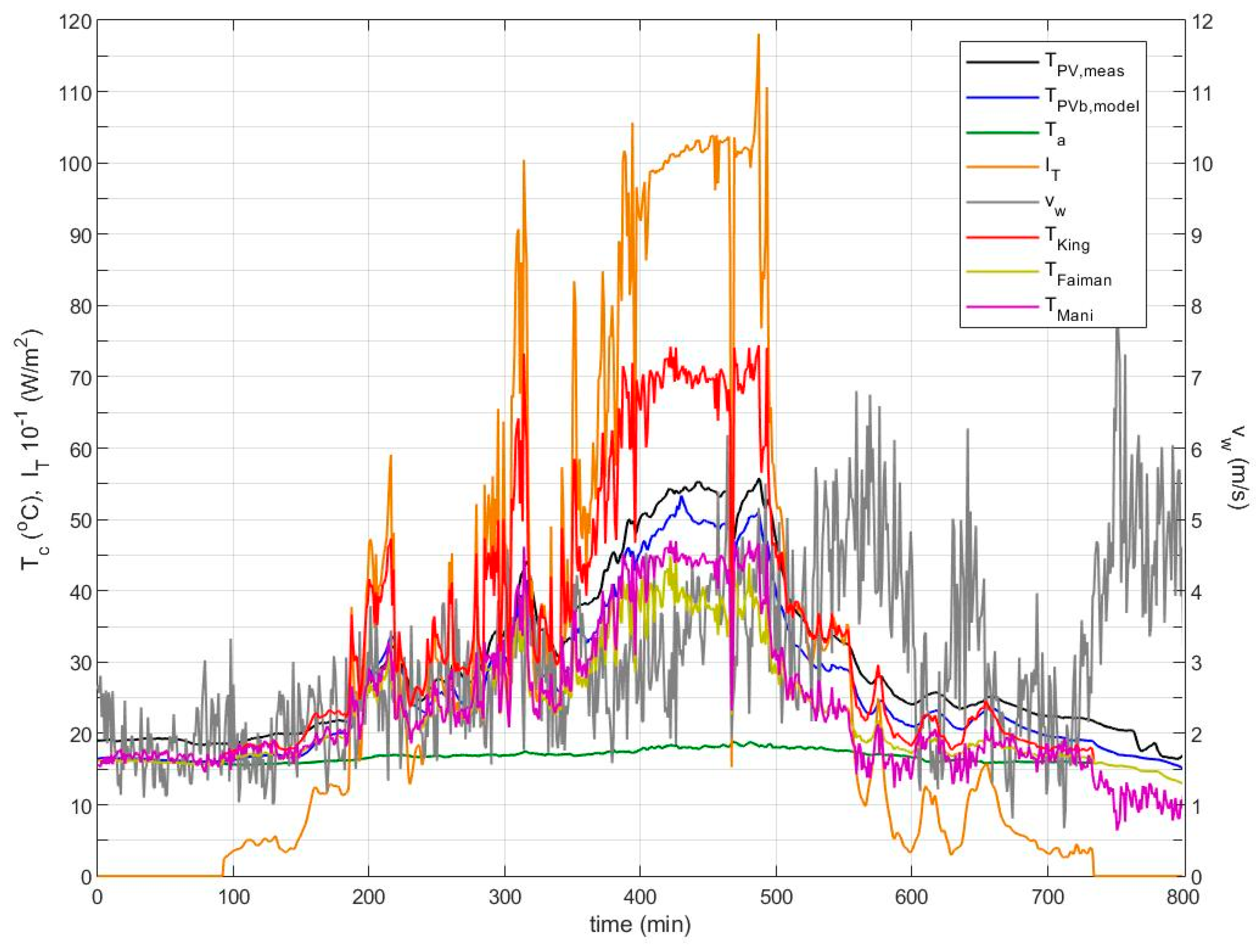
The proposed dynamic temperature prediction model is tested with the BIPV system, where transient effects can be observed at 1-min interval recordings of PV temperature for a period of 32 days across April–May–June. Figure 3 shows the predicted T_PVb profile at 1-min intervals in comparison with the PV temperature measured at the back of the module during a clear sky day in June, along with the predicted T_PVc and T_PVf profiles. The predicted T_PVb profile is in close agreement to the measured one and follows the same time pattern, which reflects the effect of the total mass heat capacity (mc_p) of the glass-EVA-cell-EVA-Tedlar which is incorporated in the transient model. The majority of the predicted values lie within 3 °C of the measured values. The high predictive capacity of the model is highlighted across the varying wind velocity, which rises from 1 m/s to spikes at 6–7 m/s with the front PV module side windward or leeward, as indicated in Figure 3.

The predicted temperature at the centre of the cell T_PVc is, on average, equal to the temperature at the back T_PVb, as expected for insulated back systems. The back PV side of the BIPV integrated in the roof experiences only natural heat convection and radiative heat exchanges with the room interior, while the front side experiences radiative exchanges with the sky and ground and heat convection natural and/or forced due to the incident wind leading to lower temperatures at the PV glass. Τhe temperature difference between the predicted T_PVc and T_PVb ranged from 0 to 0.4 °C, while the difference of the predicted T_PVc and T_PVf ranged from 0 to 2.7 °C across the entire period tested. This is in agreement with the range of values previously reported by King et al. [4] of a 0 °C temperature difference between the centre of the cell and the back surface for insulated back PV module mounting configurations.

An insight into the profiles of the convection coefficients and their influence on the predicted T_PVb profile is also provided in Figure 3. It may be observed that at instances of no wind the h_c,g-a profile is driven by natural convection, while at instances of high wind it is dominated by forced convection coinciding with h_{c,g-a (forced),} while at instances between 90–490 min, h_c,g-a is mostly governed by mixed natural and forced convection. The forced convection profile both for the windward and leeward front side was laminar, as is expected for the majority of these cases of wind flow over flat surfaces in this range of wind speeds. At the back side of the BIPV module, forced convection is not relevant, and therefore the h_c,b-a profile is only characterised by natural convection.

The sudden drop in the predicted temperature profiles at the 690 min is a result of a lower input irradiance due to shading effects on the pyranometer, before the shading also impacted the PV modules at 710 min. This is clearly shown in the drop in measured irradiance on the PV plane in Figure 4. At that time, the measured PV temperature experienced an exponential decay which is explained through Equation (23). The predicted T_PVb profile responding to the irradiance drop also follows an exponential decay whose analysis gives a time constant equal to 5.5 min. This is in agreement with the theoretically derived τ = 1/F₂ and slightly higher than the time constant 4.5 min reported in [23] for free-standing PV, as expected, since τ increases with (mc_p)_total and decreases with U.

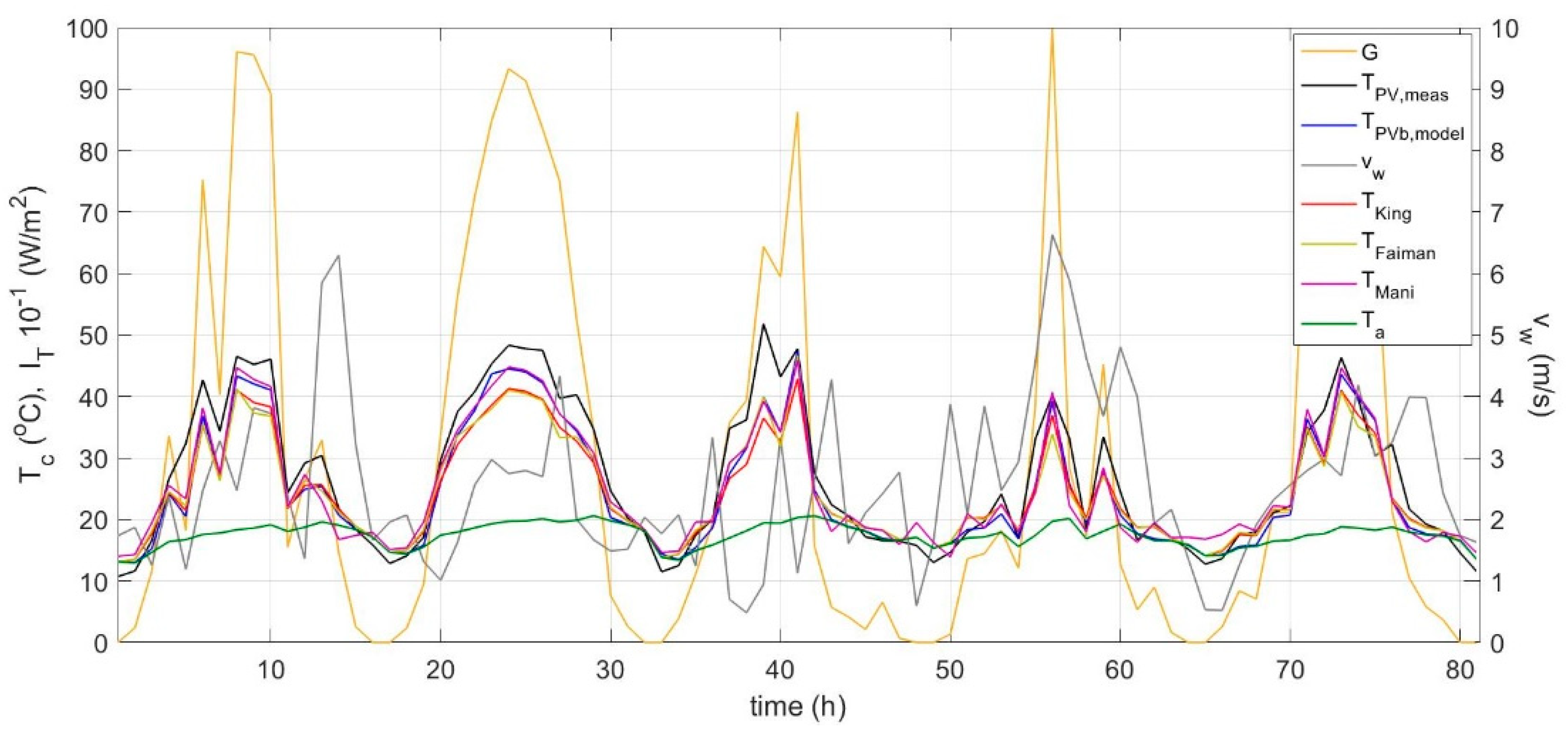
The T_PVb temperature profile predicted by this model is further compared against those obtained with the semi-empirical models by King et al. [4], Faiman [5] and the NN model by Tamizhmani et al. [10] for the same day in Figure 4. For the case of BIPV, model [4] is used with the empirical coefficients corresponding to the glass/cell/polymer sheet module with an insulated back. Figure 4 shows significant differences of up to 10–20 °C between the predicted T_PV profiles by the three models [4,5,10] and the measured T_PVmeas, which is generally more pronounced at higher wind speeds. Model [4] has a better response at higher wind speeds rather than low, while models [5,10] respond better at low wind speeds, displaying higher differences from the measured temperature at wind speeds greater than 3 m/s. The superiority of the proposed dynamic model compared to the other models is illustrated through the close agreement to the measured data across the entire range of wind speed values. 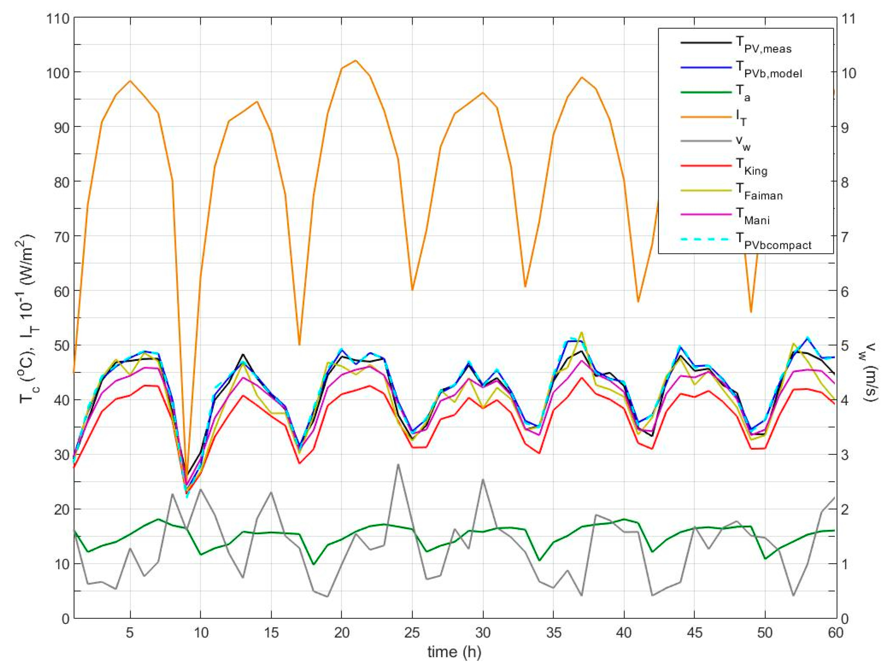Similar results are shown in Figure 5 for the performance of this model and in comparison to models [4,5,10] over 5 consecutive days in June across a wide range of wind velocities. Figure 6 and Figure 7 highlight the effectiveness of this model during cloudy and overcast days in April and for a wide range of wind velocities. The predicted vs. measured PV temperature is presented in Figure 8 illustrating an excellent agreement.

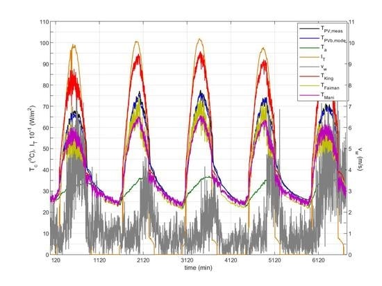
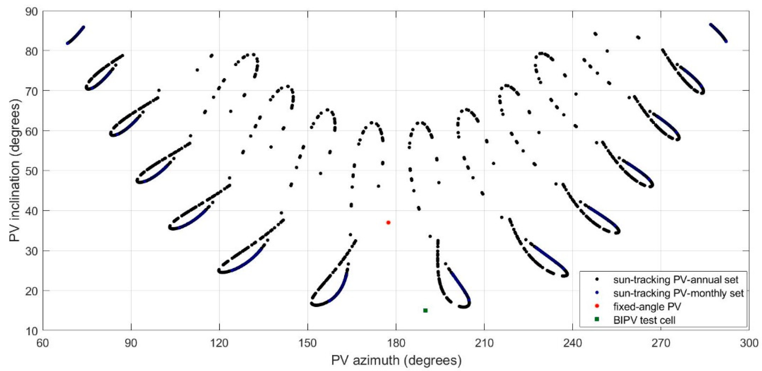
The proposed dynamic model is also tested with the free-standing PV systems, covering a wide range of PV geometries, azimuth and inclination angles, as actualised via the double-axis sun-tracking PV system, and a wide range of wind velocities during the period of 1 year at clear-sky conditions, as well as for an additional period of 1 month at varying sky conditions. In this case, the 1 h interval recordings hide the transient effects and the model response resembles that of a steady state model [22] exhibiting an improved performance over varying environmental conditions. The T_PVb predicted profiles for the sun-tracking system during a period of clear sky days and a period of partly cloudy days are shown in Figure 9 and Figure 10. The predicted profiles lie very close to the measured ones with a temperature difference in the majority of the cases throughout the year in the range of ±5 °C, and better overall performance compared to that of the models [4,5,10]. The median of the temperature difference was 0.5 °C and the 25th and 75th percentiles were −1.2 and 2.2 °C, respectively, as shown in

Table 1. ΔΤ statistics between predicted and measured values for this model and the other 3 models.

Statistic	ΔTPVb,model (°C)	ΔTKing (°C)	ΔTFaiman (°C)	ΔTMani (°C)
Median	0.5	−4.1	−3.2	−1.0
25th percentile	−1.2	−6.2	−5.4	−3.0
75th percentile	2.2	−2.3	−1.2	0.6

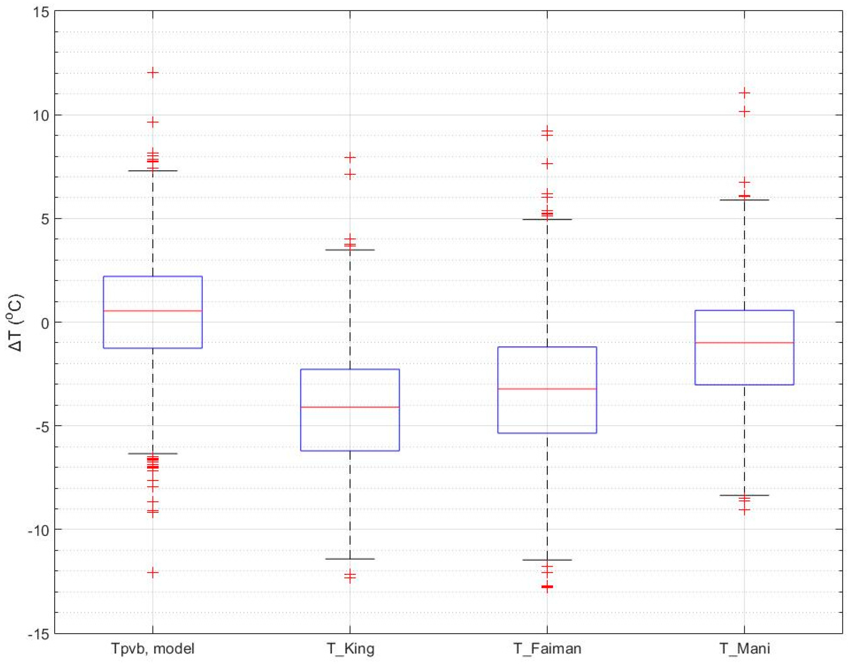
. The empirical coefficients in model [4] correspond in this case to the open rack module. Although the models [4,5,10] perform very well in the free-standing system, models [4,5] appear to under-estimate the PV temperature as shown in the boxplots in Figure 11, whereas model [10] predicts for the majority of the cases close to the measured data. A further comparison is shown in Figure 9 with the result obtained from the alternative approach using Equations (23)–(27), which shows very close results with the proposed T_PVb simulation model.

The temperature difference between the predicted T_PVc and T_PVb for the sun-tracking system ranges from 0 to 0.6 °C and the difference between T_PVc and T_PVf from 0–2.1 °C. Research studies [4,13,23,30] reported a 1–3 °C difference between the PV cell temperature and the Tedlar or the glass. While the latter is in agreement with the results of the present study, the difference between the cell centre and the Tedlar is shown to be much lower here. In [30], the glass temperature was experimentally measured and theoretically calculated to be lower than the Tedlar temperature, which is also supported by the results of the present study.

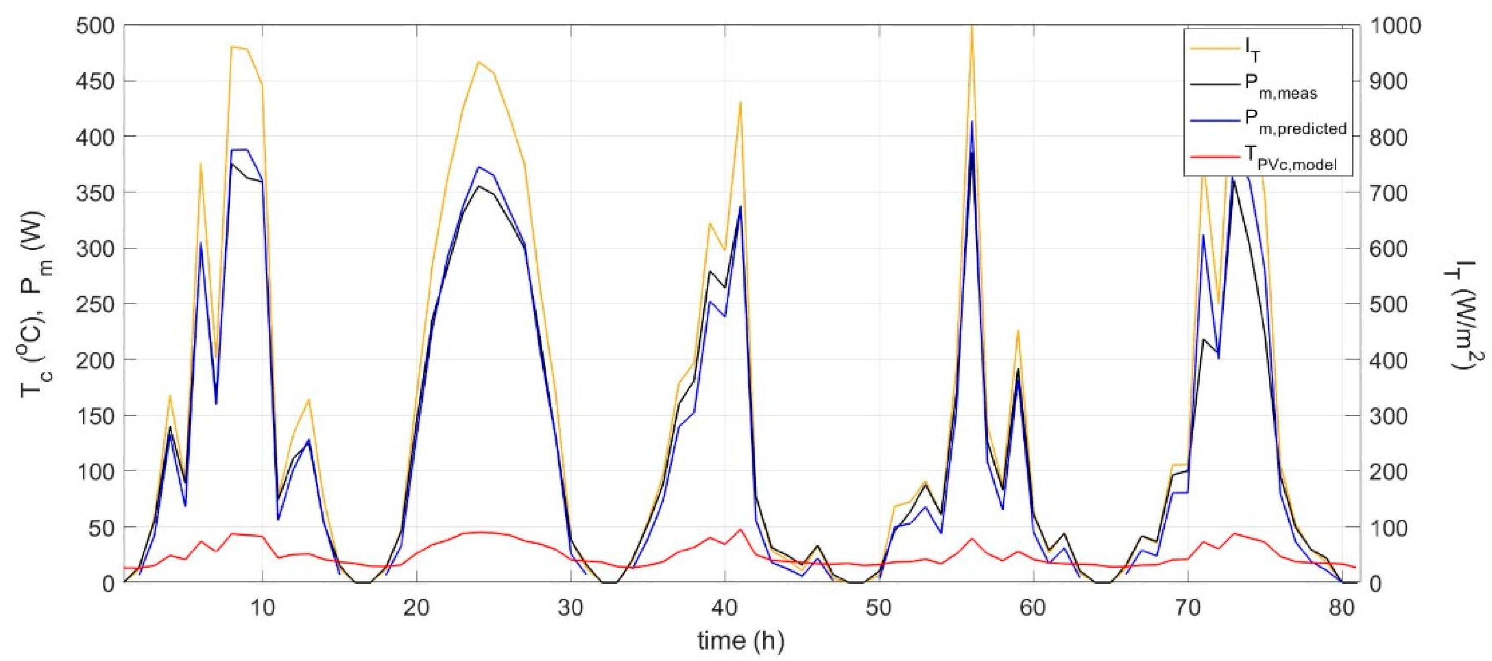
The predicted and measured temperature profiles are also examined for the fixed-angle PV system for the duration of 1 month in May covering a range of environmental conditions. Similar temperature differences were observed as with the sun-tracking system between predicted and measured PV temperature. The measured and modelled PV temperatures follow the solar irradiance profile and the impact of high wind velocities is shown to reduce both measured and predicted values (Figure 12). Based on the predicted T_PVc, the power output of the PV array is estimated from Equations (28) and (30). Power conditioning losses and further miscellaneous losses including optical losses may be additionally considered according to the system configuration. The predicted P_m profiles are compared to the measured hourly power output for the fixed-angle PV system and are shown in Figure 13. For the majority of the data, the power difference between predicted and measured lies in the range of 0–15 W, which corresponds to a deviation of less than 3.3%. This may be partly attributed to the difference between predicted and actual PV temperature at the centre of the cell. A 5 °C difference translates to 2.5% reduction in power output due to temperature alone, highlighting the importance of accurate PV temperature prediction.

The model’s predictive capacity is validated against extended experimental results of power output for the fixed-angle and the sun-tracking PV systems. The predicted vs. measured power output is displayed in Figure 14 and Figure 15 for the two systems and compared to the performance of the other models. Further analysis of the deviations between predicted and measured (ΔP_m) showed the best fit achieved through Generalized Extreme Value distribution. According to this, the model leads to a mean underestimation of power output by 1.4% in the fixed-angle system and a mean overestimation by 1.9% in the sun-tracking system. As shown in Figure 14a, the underestimation in the fixed-angle system concerns mainly lower power values and very similar results are achieved by the other models too (Figure 14b–d). In the sun-tracking system, the small overestimation occurs in the high power values, as shown in Figure 15a. Similar results are obtained with the other models exhibiting a mean underestimation by 1.2–1.4% in the fixed angle system and a mean overestimation in the range of 2.7–3.6% in the sun-tracking system. The difference in the prediction of P_m between models is 1–2%, with the proposed model exhibiting a better performance with predictions closer to the measured data.

5. Conclusions

A dynamic electro-thermal PV temperature prediction model is presented based on transient Energy Balance Equations, incorporating theoretical expressions for all heat transfer processes for both sides of the PV module, natural convection, forced convection, conduction and radiation exchanges between the module and the environment. The simulation model takes as input the environmental parameters, solar irradiance, ambient temperature, wind speed and wind direction, as well as the PV geometry parameters, PV inclination and orientation, and mounting configuration and predicts the PV temperature at the centre of the cell, the back surface and the front glass cover, the PV power output and efficiency. The algorithmic approach leads to fast convergence within 3–9 iterations. A set of equations mathematically derived from the transient EBEs is also presented, and may be alternatively used together with the complete set of theoretical expressions presented for the heat transfer processes to produce very similar results.

The model is validated with experimental data for a wide range of environmental conditions, PV geometry, and mounting configurations with data captured from a BIPV system, a double-axis sun-tracking PV, and a fixed-angle free standing PV system, and showed excellent agreement with the measured data. The transient effects were analysed through PV temperature prediction profiles for the BIPV system, and the total mass heat capacity of the glass-EVA-cell-EVA-Tedlar, together with the total energy losses coefficient, is shown to accurately predict its response. The transient model’s response to variations in the irradiance has revealed a time constant for the BIPV module of 5.5 min. The temperature difference between the centre of the cell and the back surface for all systems and conditions studied lies in the range from 0 to 0.6 °C, whereas the difference between the centre of the cell and the front glass cover in the range from 0 to 2.6 °C. The model is tested with a wide range of inclination angles ranging from 12 to 88° and orientations from 64 to 295° and the effectiveness of the model is illustrated across a range of environmental conditions, varying global and diffuse irradiance, ambient temperature, wind velocities and the windward/leeward side of the module. The median of the temperature difference between predicted and measured values was as low as 0.5 °C for the sun-tracking system, and for all cases the predicted temperature profiles closely matched the measured profiles.

Validation of the model was also carried out in terms of power output, where the predicted vs. measured PV power output proved to have excellent performance both for the fixed and the sun-tracking PV systems. Specifically, the model leads to a mean underestimation of power output by 1.4% in the fixed-angle system and a mean overestimation by 1.9% in the sun-tracking system. The difference between the predicted and measured PV power output is mainly attributed to the accuracy in the prediction of PV cell temperature and also includes ageing effects and miscellaneous optical and power losses.

The dynamic PV temperature prediction model was also compared to three well-known models, and the results showed that it has a clearly better performance and prediction capacity for a wide range of conditions and mounting configurations. The dynamic model is robust and has a firm theoretical basis, providing high accuracy and wide applicability, which may serve the needs for online PV monitoring and diagnostics and dynamic predictive management of BIPV.