Application of Waveform Stacking Methods for Seismic Location at Multiple Scales


Abstract
1. Introduction
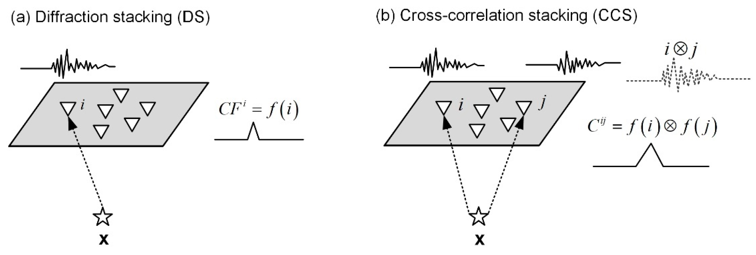
2. Methodology
3. Multiscale Field Data Examples
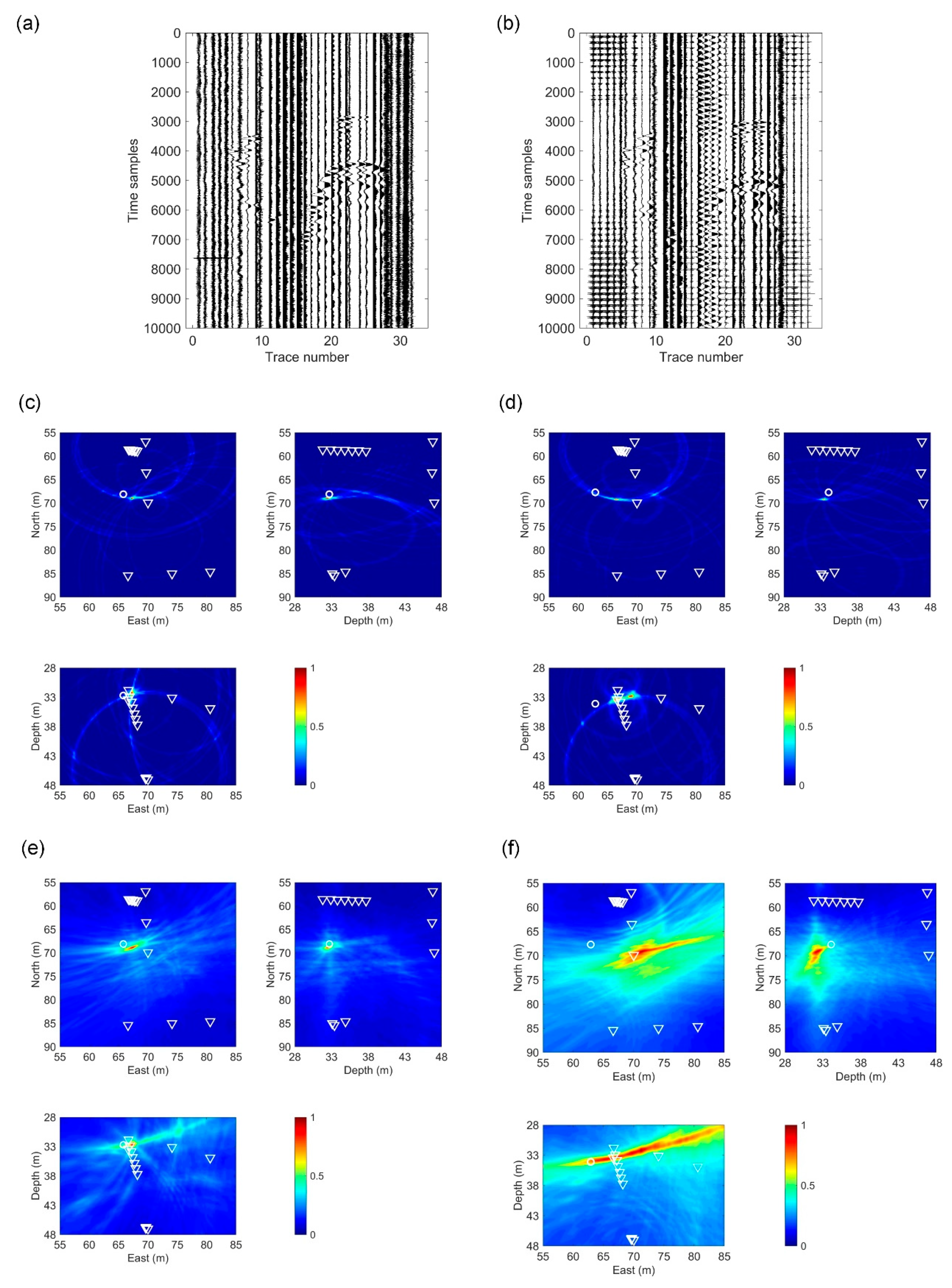
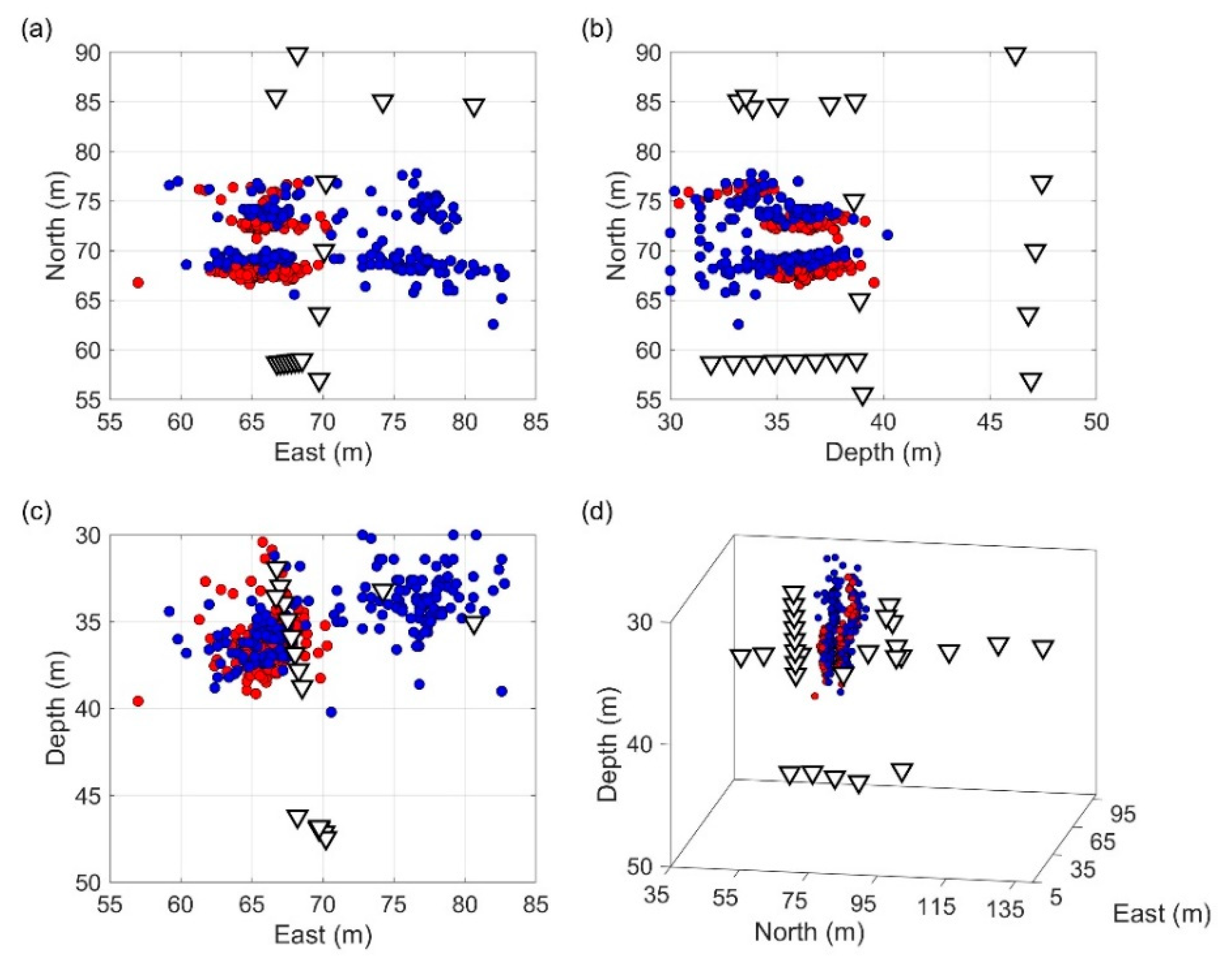
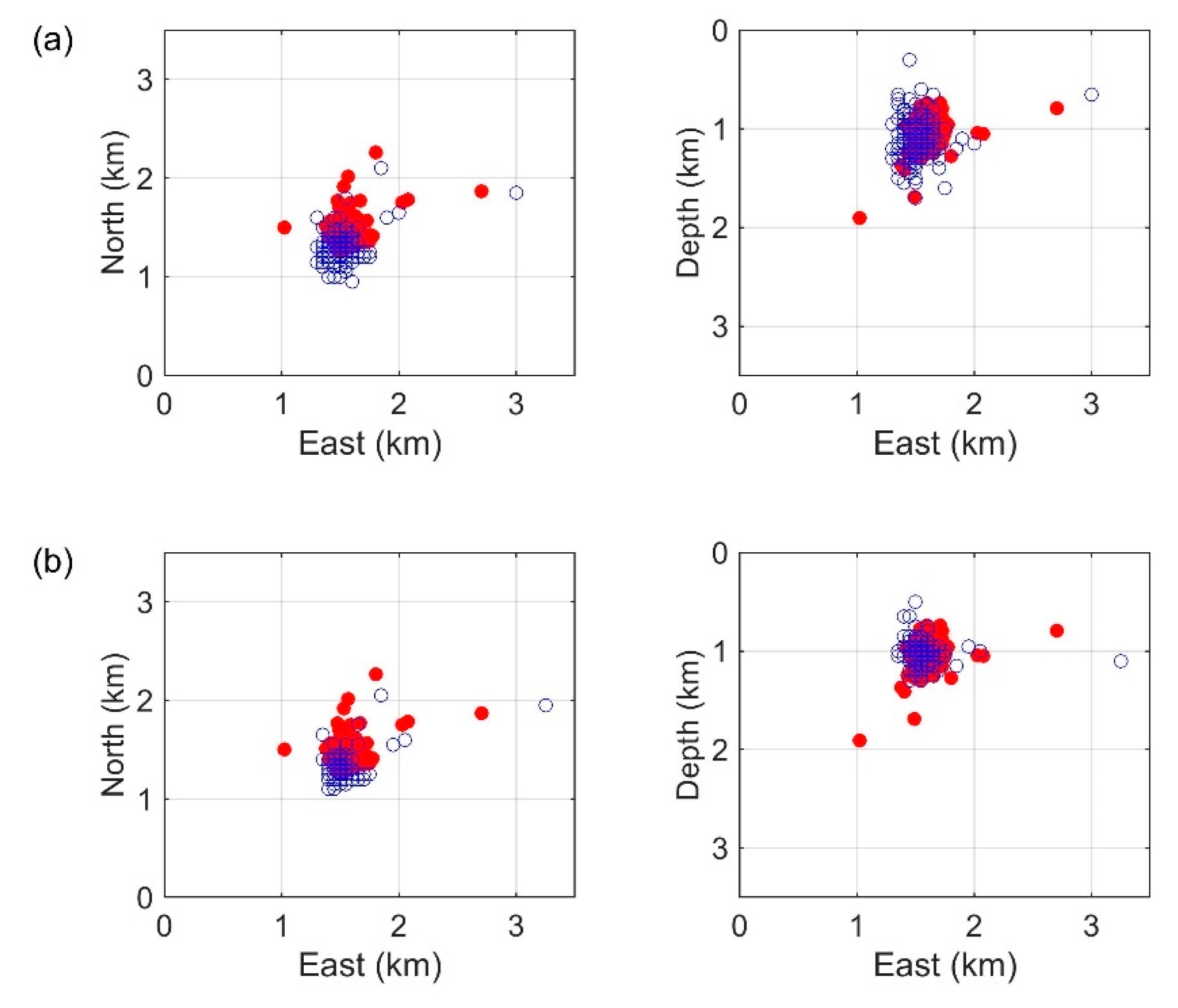
3.1. The Small-Scale Example
3.2. The Exploration-Scale Example
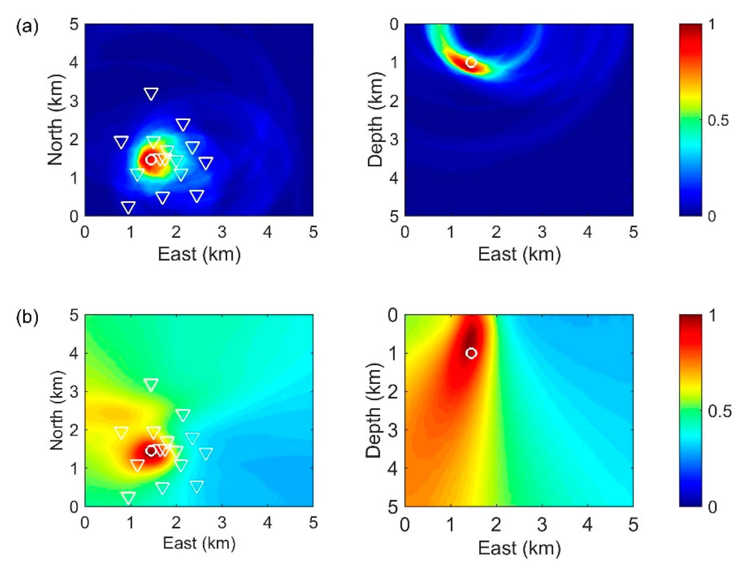
3.3. The Regional-Scale Example
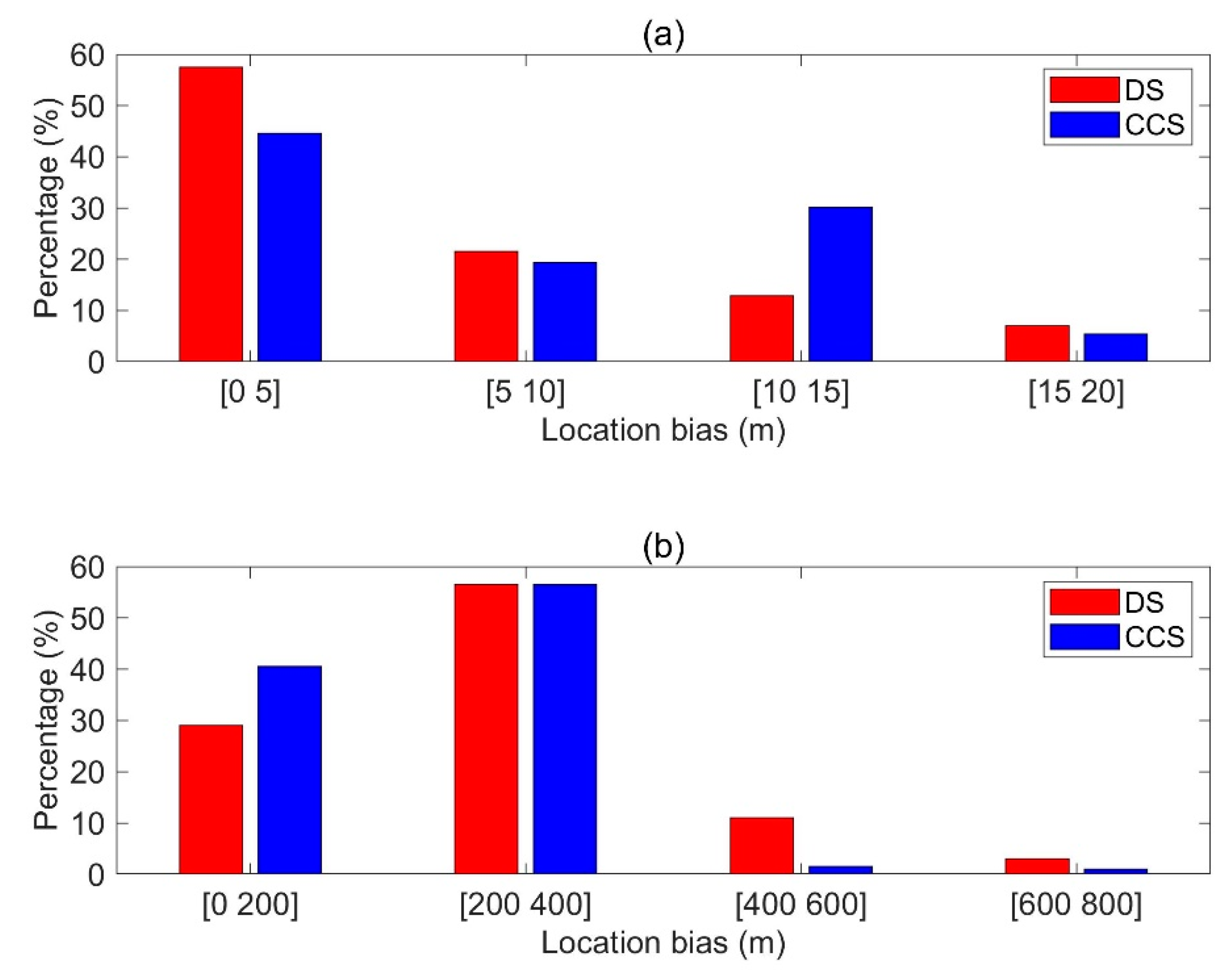
3.4. Comparison of the Results Across Scales
4. Discussion and Conclusions
Author Contributions
Funding
Acknowledgments
Conflicts of Interest
References
- Lockner, D.; Byerlee, J.D.; Kuksenko, V.; Ponomarev, A.; Sidorin, A. Quasi-static fault growth and shear fracture energy in granite. Nature 1991, 350, 39–42. [Google Scholar] [CrossRef]
- Rutqvist, J. Determination of hydraulic normal stiffness of fractures in hard rock from well testing. Int. J. Rock. Mech. Min. Geomech. Abstr. 1995, 32, 513–523. [Google Scholar] [CrossRef]
- Gibowicz, S.J.; Kijko, A. An Introduction to Mining Seismology; Academic Press: San Diego, CA, USA, 1994; ISBN 978-0-12-282120-2. [Google Scholar]
- Mendecki, A.J. (Ed.) Seismic Monitoring in Mines, 1st ed.; Chapman & Hall: London, UK, 1997; ISBN 978-0-412-75300-8. [Google Scholar]
- Luo, X.; Hatherly, P. Application of microseismic monitoring to characterise geomechanical conditions in longwall mining. Explor. Geophys. 1998, 29, 489–493. [Google Scholar] [CrossRef]
- Maxwell, S.C. Microseismic Imaging of Hydraulic Fracturing; Distinguished Instructor Series; Society of Exploration Geophysicists: Tulsa, OK, USA, 2014; ISBN 978-1-56080-315-7. [Google Scholar]
- Grigoli, F.; Cesca, S.; Priolo, E.; Rinaldi, A.P.; Clinton, J.F.; Stabile, T.A.; Dost, B.; Fernandez, M.G.; Wiemer, S.; Dahm, T. Current challenges in monitoring, discrimination, and management of induced seismicity related to underground industrial activities: A European perspective. Rev. Geophys. 2017, 55, 310–340. [Google Scholar] [CrossRef]
- Eaton, D.W. Passive Seismic Monitoring of Induced Seismicity: Fundamental Principles and Application to Energy Technologies, 1st ed.; Cambridge University Press: Cambridge, UK, 2018; ISBN 978-1-107-14525-2. [Google Scholar]
- Li, L.; Tan, J.; Wood, D.A.; Zhao, Z.; Becker, D.; Lyu, Q.; Shu, B.; Chen, H. A review of the current status of induced seismicity monitoring for hydraulic fracturing in unconventional tight oil and gas reservoirs. Fuel 2019, 242, 195–210. [Google Scholar] [CrossRef]
- Shearer, P.M. Introduction to Seismology, 2nd ed.; Cambridge University Press: Cambridge, UK, 2009; ISBN 978-0-521-70842-5. [Google Scholar]
- Thurber, C.H.; Rabinowitz, N. Advances in Seismic Event Location; Springer: Dordrecht, The Netherlands, 2000; ISBN 978-90-481-5498-2. [Google Scholar]
- Lomax, A.; Michelini, A.; Curtis, A. Earthquake Location, Direct, Global-Search Methods. In Encyclopedia of Complexity and Systems Science; Meyers, R.A., Ed.; Springer: New York, NY, USA, 2009; pp. 2449–2473. ISBN 978-0-387-75888-6. [Google Scholar]
- Li, L.; Tan, J.; Schwarz, B.; Staněk, F.; Poiata, N.; Shi, P.; Diekmann, L.; Eisner, L.; Gajewski, D. Recent advances and challenges of waveform-based seismic location methods at multiple scales. Rev. Geophys. 2020, 58, e2019RG000667. [Google Scholar] [CrossRef]
- Dong, L.; Hu, Q.; Tong, X.; Liu, Y. Velocity-Free MS/AE Source Location Method for Three-Dimensional Hole-Containing Structures. Engineering 2020, in press. [Google Scholar] [CrossRef]
- Peng, P.; Jiang, Y.; Wang, L.; He, Z. Microseismic Event Location by Considering the Influence of the Empty Area in an Excavated Tunnel. Sensors 2020, 20, 574. [Google Scholar] [CrossRef]
- Cesca, S.; Grigoli, F. Chapter two-full waveform seismological advances for microseismic monitoring. Adv. Geophys. 2015, 56, 169–228. [Google Scholar]
- Trojanowski, J.; Eisner, L. Comparison of migration-based location and detection methods for microseismic events. Geophys. Prospect. 2017, 65, 47–63. [Google Scholar] [CrossRef]
- Beskardes, G.D.; Hole, J.A.; Wang, K.; Michaelides, M.; Wu, Q.; Chapman, M.C.; Davenport, K.K.; Brown, L.D.; Quiros, D.A. A comparison of earthquake backprojection imaging methods for dense local arrays. Geophys. J. Int. 2018, 212, 1986–2002. [Google Scholar] [CrossRef]
- Kao, H.; Shan, S.J. The source-scanning algorithm: Mapping the distribution of seismic sources in time and space. Geophys. J. Int. 2004, 157, 589–594. [Google Scholar] [CrossRef]
- Baker, T.; Granat, R.; Clayton, R.W. Real-time earthquake location using Kirchhoff reconstruction. Bull. Seismol. Soc. Am. 2005, 95, 699–707. [Google Scholar] [CrossRef]
- Gajewski, D.; Anikiev, D.; Kashtan, B.; Tessmer, E. Localization of seismic events by diffraction stacking. In Proceedings of the SEG Technical Program Expanded Abstracts, San Antonio, TX, USA, 23–28 September 2007; Society of Exploration Geophysicists: Tulsa, OK, USA, 2007; pp. 1287–1291. [Google Scholar]
- Schuster, G.T.; Yu, J.; Sheng, J. Interferometric/daylight seismic imaging. Geophys. J. Int. 2004, 157, 838–852. [Google Scholar] [CrossRef]
- Xiao, X.; Luo, Y.; Fu, Q.; Jervis, M.; Dasgupta, S.; Kelamis, P. Locate microseismicity by seismic interferometry. In Proceedings of the Second EAGE Passive Seismic Workshop-Exploration and Monitoring Applications, Limassol, Cyprus, 22–25 March 2009; The European Association of Geoscientists and Engineers: Houten, The Netherlands, 2009; p. A22. [Google Scholar]
- Li, L.; Chen, H.; Wang, X.-M. Weighted-elastic-wave interferometric imaging of microseismic source location. Appl. Geophy. 2015, 12, 221–234. [Google Scholar] [CrossRef]
- Kiselevitch, V.L.; Nikolaev, A.V.; Troitskiy, P.A.; Shubik, B.M. Emission tomography: Main ideas, results, and prospects. In Proceedings of the SEG Technical Program Expanded Abstracts, Houston, TX, USA, 10–14 September 1991; Society of Exploration Geophysicists: Tulsa, OK, USA, 1991; p. 1602. [Google Scholar]
- Duncan, P.M. Is there a future for passive seismic? First Break 2005, 23, 111–115. [Google Scholar]
- Anikiev, D.; Valenta, J.; Staněk, F.; Eisner, L. Joint location and source mechanism inversion of microseismic events: Benchmarking on seismicity induced by hydraulic fracturing. Geophys. J. Int. 2014, 198, 249–258. [Google Scholar] [CrossRef]
- Poiata, N.; Satriano, C.; Vilotte, J.-P.; Bernard, P.; Obara, K. Multiband array detection and location of seismic sources recorded by dense seismic networks. Geophys. J. Int. 2016, 205, 1548–1573. [Google Scholar] [CrossRef]
- Grigoli, F.; Cesca, S.; Vassallo, M.; Dahm, T. Automated Seismic Event Location by Travel-Time Stacking: An Application to Mining Induced Seismicity. Seismol. Res. Lett. 2013, 84, 666–677. [Google Scholar] [CrossRef]
- Li, L.; Becker, D.; Chen, H.; Wang, X.; Gajewski, D. A systematic analysis of correlation-based seismic location methods. Geophys. J. Int. 2018, 212, 659–678. [Google Scholar] [CrossRef]
- Shi, P.; Nowacki, A.; Rost, S.; Angus, D. Automated seismic waveform location using Multichannel Coherency Migration (MCM)—II. Application to induced and volcano-tectonic seismicity. Geophys. J. Int. 2019, 216, 1608–1632. [Google Scholar] [CrossRef]
- Zhang, C.; Qiao, W.; Che, X.; Lu, J.; Men, B. Automated microseismic event location by amplitude stacking and semblance. Geophysics 2019, 84, KS191–KS210. [Google Scholar] [CrossRef]
- Pesicek, J.D.; Child, D.; Artman, B.; Cieślik, K. Picking versus stacking in a modern microearthquake location: Comparison of results from a surface passive seismic monitoring array in Oklahoma. Geophysics 2014, 79, KS61–KS68. [Google Scholar] [CrossRef]
- Staněk, F.; Anikiev, D.; Valenta, J.; Eisner, L. Semblance for microseismic event detection. Geophys. J. Int. 2015, 201, 1362–1369. [Google Scholar] [CrossRef]
- Gharti, H.N.; Oye, V.; Roth, M.; Kühn, D. Automated microearthquake location using envelope stacking and robust global optimization. Geophysics 2010, 75, MA27–MA46. [Google Scholar] [CrossRef]
- Zhang, W.; Zhang, J. Microseismic migration by semblance-weighted stacking and interferometry. In Proceedings of the SEG Technical Program Expanded Abstracts, Houston, TX, USA, 22–27 September 2013; Society of Exploration Geophysicists: Tulsa, OK, USA, 2013; pp. 2045–2049. [Google Scholar]
- Grigoli, F.; Scarabello, L.; Böse, M.; Weber, B.; Wiemer, S.; Clinton, J.F. Pick-and waveform-based techniques for real-time detection of induced seismicity. Geophys. J. Int. 2018, 213, 868–884. [Google Scholar] [CrossRef]
- Langet, N.; Maggi, A.; Michelini, A.; Brenguier, F. Continuous Kurtosis-Based Migration for Seismic Event Detection and Location, with Application to Piton de la Fournaise Volcano, La Reunion. Bull. Seismol. Soc. Am. 2014, 104, 229–246. [Google Scholar] [CrossRef]
- Li, L.; Tan, J.; Xie, Y.; Tan, Y.; Walda, J.; Zhao, Z.; Gajewski, D. Waveform-based microseismic location using stochastic optimization algorithms: A parameter tuning workflow. Comput. Geosci. 2019, 124, 115–127. [Google Scholar] [CrossRef]
- Amann, F.; Gischig, V.; Evans, K.; Doetsch, J.; Jalali, R.; Valley, B.; Krietsch, H.; Dutler, N.; Villiger, L.; Brixel, B.; et al. The seismo-hydromechanical behavior during deep geothermal reservoir stimulations: Open questions tackled in a decameter-scale in situ stimulation experiment. Solid Earth 2018, 9, 115–137. [Google Scholar] [CrossRef]
- Gischig, V.S.; Doetsch, J.; Maurer, H.; Krietsch, H.; Amann, F.; Evans, K.F.; Nejati, M.; Jalali, M.; Valley, B.; Obermann, A.C.; et al. On the link between stress field and small-scale hydraulic fracture growth in anisotropic rock derived from microseismicity. Solid Earth 2018, 9, 39–61. [Google Scholar] [CrossRef]
- Cook, N.G.W. Seismicity associated with mining. Eng. Geol. 1976, 10, 99–122. [Google Scholar] [CrossRef]
- Zhang, H.; Chen, L.; Chen, S.; Sun, J.; Yang, J. The Spatiotemporal Distribution Law of Microseismic Events and Rockburst Characteristics of the Deeply Buried Tunnel Group. Energies 2018, 11, 3257. [Google Scholar] [CrossRef]
- Feng, G.; Xia, G.; Chen, B.; Xiao, Y.; Zhou, R. A Method for Rockburst Prediction in the Deep Tunnels of Hydropower Stations Based on the Monitored Microseismicity and an Optimized Probabilistic Neural Network Model. Sustainability 2019, 11, 3212. [Google Scholar] [CrossRef]
- Bischoff, S.T.; Fischer, L.; Wehling-Benatelli, S.; Fritschen, R.; Meier, T.; Friederich, W. Spatio-Temporal Characteristics of Mining Induced Seismicity in the Eastern Ruhr-Area; The European Center for Geodynamics and Seismology (ECGS): Walferdange, Luxembourg, 2010. [Google Scholar]
- Ellsworth, W.L. Injection-induced earthquakes. Science 2013, 341, 1225942. [Google Scholar] [CrossRef]
- Dougherty, S.L.; Cochran, E.S.; Harrington, R.M. The LArge-n Seismic Survey in Oklahoma (LASSO) Experiment. Seismol. Res. Lett. 2019, 90, 2051–2057. [Google Scholar] [CrossRef]
- Rubinstein, J.L.; Ellsworth, W.L.; Dougherty, S.L. The 2013–2016 Induced Earthquakes in Harper and Sumner Counties, Southern Kansas. Bull. Seismol. Soc. Am. 2018, 108, 674–689. [Google Scholar] [CrossRef]
- Eisner, L.; Duncan, P.M.; Heigl, W.M.; Keller, W.R. Uncertainties in passive seismic monitoring. Leading Edge 2009, 28, 648–655. [Google Scholar] [CrossRef]
- Ruigrok, E.; Gibbons, S.; Wapenaar, K. Cross-correlation beamforming. J. Seismol. 2017, 21, 495–508. [Google Scholar] [CrossRef]
- López-Comino, J.A.; Cesca, S.; Heimann, S.; Grigoli, F.; Milkereit, C.; Dahm, T.; Zang, A. Characterization of hydraulic fractures growth during the Äspö Hard Rock laboratory experiment (Sweden). Rock Mech. Rock Eng. 2017, 50, 2985–3001. [Google Scholar] [CrossRef]
- Guidarelli, M.; Klin, P.; Priolo, E. Migration-based near real-time detection and location of microearthquakes with parallel computing. Geophys. J. Int. 2020, 221, 1941–1958. [Google Scholar] [CrossRef]
- Lee, E.-J.; Liao, W.-Y.; Mu, D.; Wang, W.; Chen, P. GPU-Accelerated Automatic Microseismic Monitoring Algorithm (GAMMA) and Its Application to the 2019 Ridgecrest Earthquake Sequence. Seismol. Res. Lett. 2020, in press. [Google Scholar] [CrossRef]


| Parameters | Small Scale | Exploration Scale | Regional Scale |
|---|---|---|---|
| Receiver channel | 32 × 3 | 15 × 3 | approx. 1800 × 1 |
| Number of events | 186 | 200 | 2 |
| Sampling rate | 1 MHz | 200 Hz | 500 Hz |
| Target volume | 30 m × 35 m× 20 m | 5 km × 5 km× 5 km | 35.2 km × 45.2 km × 8 km |
| Velocity model | homogeneous isotropic | homogeneous isotropic | layered isotropic |
| Grid spacing | 1 m | 50 m | 400 m |
| Band-pass filter | 1–50 kHz | 5–30 Hz | / |
| Length of short-/long-term window | 80/160 | 25/50 | 25/50 |
| Location Bias | Small Scale | Exploration Scale | Regional Scale | |
|---|---|---|---|---|
| DS | E-direction (m) | 5.056 | 94.85 | 729.5 |
| N-direction (m) | 1.854 | 163.64 | 182.5 | |
| Z-direction (m) | 1.689 | 172.68 | 1675.5 | |
| Overall (m) | 6.156 | 281.59 | 1909.4 | |
| CCS | E-direction (m) | 6.513 | 72.20 | 156.5 |
| N-direction (m) | 1.268 | 165.51 | 560.5 | |
| Z-direction (m) | 1.799 | 122.11 | 1675.5 | |
| Overall (m) | 7.154 | 236.10 | 1782.8 | |
© 2020 by the authors. Licensee MDPI, Basel, Switzerland. This article is an open access article distributed under the terms and conditions of the Creative Commons Attribution (CC BY) license (http://creativecommons.org/licenses/by/4.0/).
Share and Cite
Li, L.; Xie, Y.; Tan, J. Application of Waveform Stacking Methods for Seismic Location at Multiple Scales. Energies 2020, 13, 4729. https://doi.org/10.3390/en13184729
Li L, Xie Y, Tan J. Application of Waveform Stacking Methods for Seismic Location at Multiple Scales. Energies. 2020; 13(18):4729. https://doi.org/10.3390/en13184729
Chicago/Turabian StyleLi, Lei, Yujiang Xie, and Jingqiang Tan. 2020. "Application of Waveform Stacking Methods for Seismic Location at Multiple Scales" Energies 13, no. 18: 4729. https://doi.org/10.3390/en13184729
APA StyleLi, L., Xie, Y., & Tan, J. (2020). Application of Waveform Stacking Methods for Seismic Location at Multiple Scales. Energies, 13(18), 4729. https://doi.org/10.3390/en13184729