Prognostics and Health Management for the Optimization of Marine Hybrid Energy Systems

Abstract

Decarbonization of marine transport is a key global issue, with the carbon emissions of international shipping projected to increase 23% to 1090 million tonnes by 2035 in comparison to 2015 levels. Optimization of the energy system (especially propulsion system) in these vessels is a complex multi-objective challenge involving economical maintenance, environmental metrics, and energy demand requirements. In this paper, data from instrumented vessels on the River Thames in London, which includes environmental emissions, power demands, journey patterns, and variance in operational patterns from the captain(s) and loading (passenger numbers), is integrated and analyzed through automatic, multi-objective global optimization to create an optimal hybrid propulsion configuration for a hybrid vessel. We propose and analyze a number of computational techniques, both for monitoring and remaining useful lifetime (RUL) estimation of individual energy assets, as well as modeling and optimization of energy use scenarios of a hybrid-powered vessel. Our multi-objective optimization relates to emissions, asset health, and power performance. We show that, irrespective of the battery packs used, our Relevance Vector Machine (RVM) algorithm is able to achieve over 92% accuracy in remaining useful life (RUL) predictions. A k-nearest neighbors algorithm (KNN) is proposed for prognostics of state of charge (SOC) of back-up lead-acid batteries. The classifier achieved an average of 95.5% accuracy in a three-fold cross validation. Utilizing operational data from the vessel, optimal autonomous propulsion strategies are modeled combining the use of battery and diesel engines. The experiment results show that 70% to 80% of fuel saving can be achieved when the diesel engine is operated up to 350 kW. Our methodology has demonstrated the feasibility of combination of artificial intelligence (AI) methods and real world data in decarbonization and optimization of green technologies for maritime propulsion.

1. Introduction

Global marine transport is a vital contributor to the economy, supporting the transfer of goods and people throughout the world. As a result, marine transport is a significant and growing consumer of energy and fuel consumption. According to a report by the Organization for Economic Co-operation and Development (OECD), carbon emissions from global shipping are projected to reach approximately 1090 million tonnes by 2035, representing a 23% growth from 2015 [1]. The main driver behind such growth is the rise in international trade. Emissions have reduced during the global lock-down as result of Covid-19; however, a rebound effect in carbon emissions will resume when restrictions are removed [2]. The combination of climate change and the forecasted global recession further increases the demand for economical decarbonization solutions that can be applied to existing fleets.

In 2014, the European Environment Agency also found that most of the energy consumption growth within the core EU-13 countries came from marine transport [3]. Approximately 80% of world merchandise trade is carried over by water, with marine trade reaching nearly 60 trillion ton-miles [4]. In the United Kingdom, approximately 95% of the country’s imports and exports in goods are moved by sea, including almost half of the country’s food supplies [5]. Energy demand from marine freight is expected to increase by 6 quadrillion Btu [6].

Marine transportation relies on fossil-fueled vessels that produce harmful emissions, such as sulfur dioxide (SO${}_2$), nitrogen oxides (NO${}_{\mathrm{x}}$), and carbon dioxide (CO${}_2$) emissions. The UK Department of Transport reported that, as of 2016, domestic shipping alone accounted for 11% of the UK’s domestic NO${}_{\mathrm{x}}$ emissions [5]. In 2017, the UK domestic shipping accounted for 5.9 Mt of CO${}_2$ equivalent, with domestic and international shipping, combined, responsible for 13.87 Mt of CO${}_2$ equivalent [7]. Internationally, the shipping industry contributed 15% to global NO${}_{\mathrm{x}}$ emissions in 2014 alone [8].

If no measures are taken to advance propulsion systems and improve their operational efficiency, CO${}_2$ emissions are projected to increase between 50% to 250% in 2050. According to the UK Marine Industries Alliance (MIA), it is essential that the marine industry develop energy-efficient, environmentally friendly, and cost-effective vessels [9]. To enforce such advancement on a global scale, the International Marine Organization (IMO) Marpol regulations implemented limitations on sulfur and NO${}_{\mathrm{x}}$ emissions for diesel engines with outputs higher than 130 kW. Such regulatory initiatives create demand for alternative and more efficient ways of energy use [6] and consideration of electric or hybrid-propulsion vessels. However, it is worth noting that any attempts in decarbonization need to factor in economical and legacy fleet issues, due to the fact that a significant share of current ships will still be in operation by 2035 [1].

To achieve improvements in fuel-efficiency and a reduction in emissions, hybrid diesel-electric power systems have been adopted increasingly within the marine industry [10]. A typical hybrid vessel employs fossil-fuelled engines and lithium-ion batteries for power. Meanwhile, lead-acid batteries are used as a stand-by power source. Different from fuel-only propulsion, the hybrid propulsion system allows the vessel to reduce fuel consumption and fuel costs [11]. The American Navy vessel, Makin Island, employed electric motors as part of its propulsion system and saved over a million gallons of diesel on its maiden cruise, representing a $2.2$ million fuel cost reduction [12]. Hybrid vessels also benefit from decreased emissions compared to fuel-only vessels [11].

Propulsion assets are essential to every aspect of vessel operations, therefore, operators must be confident that lithium-ion batteries can reliably provide sufficient propulsion power when the diesel engine is on stand-by mode. These on-board batteries are rechargeable, but chemical reactions that take place inside the batteries will inevitably lead to cell-aging and capacity degradation [13,14,15], especially at high power outputs as required for vessel propulsion. As a result of this, reliable condition monitoring of lithium-ion batteries is crucial to support safe operation of vessels and protect the availability of energy services. Similarly, lead-acid batteries have been widely deployed within the marine industry. Lead-acid batteries were primarily installed for uninterruptible power supply (UPS) services [16]. In the event of a loss of generator power, lead-acid batteries allow ships to continue to operate until primary power is restored. Although lead-acid batteries are not used to provide primary propulsion power, capacity degradation due to aging occurs and consequently compromises the vessel’s ability to operate [17].

A critical asset on a hybrid vessel is the diesel engine, the lifetime of a diesel engine could be as long as 20 years, as in Reference [18]. However, the actual lifespan is directly influenced by its operational usage. Furthermore, its performance if operating at part load and outwith of its optimal design and operation points, will be associated with increased fuel consumption and emissions [19]. Therefore, maintenance and health management strategies related to actual usage of a diesel engine is essential to ensure optimal operation of vessels, and prevent downtime of the vessel [20]. Current health management strategies for diesel engines rely on time based (scheduled) maintenance. This maintenance regime is traditionally based on prior learning and historical statistical analysis. By not using real-time data to inform these schedules, both technical and commercial risks are incurred, such as incorrect or incomplete maintenance, induced damage through intervention, impacts of new load patterns, unnecessary non-productive time, and early replacement of healthy components [21]. Consequently, more advanced asset health management systems for hybrid vessel are required that take into account the dynamics that exist in these complex systems. Current literature on intelligent asset health management tends to focus on prognostics of single-type assets [22,23,24,25] or using simulated data to test the reliability of health management models [26,27]. A gap exists in the literature for the analysis of the complex dynamic relationships between multiple assets that simultaneously respond to the needs of vessels in real-world environments. Run-time optimization of sub-systems whilst meeting operational objectives, optimally, during dynamic loading and ambient conditions represents a significant challenge. Through a detailed optimization, balancing the usage and optimal performance characteristics of the diesel engine and lithium-ion battery, the lifespan of the diesel engine and lithium-ion batteries can be positively affected [28]. Therefore, it is crucial to identify the conditions under which diesel engines operate sub-optimally and inefficiently. In doing so, hybrid vessel operators can switch or combine diesel and electric propulsion power, simultaneously, to maximize fuel efficiency and reduce emissions of the vessels.

In the context of the current state of the art, our research addresses several key knowledge gaps. First, using operational and other test data, we create prognostic models for state of health estimation of individual energy subsystems present aboard a hybrid-powered vessel-specifically, Li-ion and lead-acid batteries. Second, we optimize the diesel engine performance in the presence of lithium-ion battery assets, as part of a hybrid propulsion system. Third, through the use of multi-objective optimization which includes asset health, energy performance and environmental metrics, examine a number of control methods which can be used in the operation of an autonomous energy management system. These findings capture the inter-dependencies and variances in real-world operations and overcome the limitations of data from simulated marine vessel performance.

The remainder of this paper is organized as follows: Section 2 presents an overview on prognostics and health management (PHM) and research into the propulsion of marine vessels. Section 3 describes our approach of optimization and the data sources utilized within this study, while Section 4 presents our methodology and results for individual asset forecasts within a hybrid energy system, e.g., Li-on battery, lead-acid battery and diesel engine. Section 5 provides an description of the whole system optimization for the hybrid energy system, and demonstrates the effect of autonomous energy system management for a hybrid propulsion system under different operating scenarios. Finally, Section 6 summarizes the key observations from results and recommendations from our findings, as well as suggestions for future work.

2. Prognostics and Propulsion Research in Marine Systems

Within this section, we provide a brief overview of prognostic health management and propulsion research with reference to components and sub-systems relevant to hybrid marine vessels.

2.1. Prognostics and Health Management

Remaining useful life (RUL) is the length of time an asset, e.g., component, sub-system, or system, is likely to operate before it requires repair or replacement. The estimation of the RUL of components, sub-systems and systems, traditionally relies on analysis of data, which contains signatures of failure modes, collated over a systems’ life cycle. Such data can be scarce and difficult to obtain due to the sensitivities of companies releasing such data, or due to the early replacement of assets. Reliability based RUL estimation relies on understanding the failure characteristics of the asset and determines what can be done to manage the consequence of the failure [29,30].

A common approach when failure data is available is to fit a Weibull distributions to this failure data. However, as shown by Turner [31], there are significant limitations to this approach, such as: (1) lack of reliable data, (2) influence of multiple failure mechanisms of an engineering system, and (3) component failure distribution does not match the Weibull distribution. Statistical analysis often ignores the mechanism of failure or assumes only one failure mechanism, which is not the case in many complex engineering systems, and results in fixed time replacement of components. In comparison, a prognostic approach aims at predicting failure based on individual component state estimation by employing either physics of failure, data or fusion degradation models [32].

Prognostics and Health Management (PHM) is a highly multidisciplinary field that aims to forecast asset failures ahead of time in order to enable intelligent health management whilst the system remains in operation [33]. The main purpose of a prognostic model is to detect system state deviation from a healthy baseline state by understanding whether the engineering system is behaving within nominal operational bounds [34].

There are three main approaches to prognostics: A statistical, reliability-based PHM approach which assumes usage and environmental conditions have no effect and that knowledge of the failure mechanism is not required [35]. A physical, modeling-based approach that mimics the component or system deterioration/decay via nominal life models. This can include degradation models or damage accumulation models based on failure modes mechanism, such as wear, fatigue, corrosion, and contamination [14]. On the other hand, the data-driven prognostics approach is an application of machine learning and statistical pattern recognition on data collected at system, subsystem or component level [32,36]. In practice, a prognostics architecture can rely on an individual method or a combination of the three. The selection of method depends on available data, previous models and system physical knowledge. Although PHM methods have been widely used across numerous industries on machinery, electronics, avionic systems, and vehicles with great success, challenges still persist in creating accurate models from imperfect real-world operational data and in producing predictions within time-critical and operational timescales. For example, real-world operational data are collected on different vessels, settings, and under different contexts. Existing data may not be suitable for our analysis without knowing full details of the data collection process. Second, data related to failure modes and faults need to be sufficient for training models; in some cases, such as for standby assets, it may be difficult to obtain sufficient hazard/failure related operational data [37]. Representativeness of the data is also a concern, as data collected may not be fully representative of all operation conditions. As a result, prognostics using these data may lead to false positive predictions [38]. In practice, it may be time-consuming for users to collect representative data, and they may be reluctant to use PHM applications due to this delay. In addition, due to the complexity in modeling single assets, system of system level prognostics is still in its early stages of research and development.

2.2. Propulsion and Health Management of Marine Vessels

In Reference [39], the marine transport optimization problem is focused on the ships voyage where emissions, cruising distance and cruising speed constraints are fulfilled in multiple stages. However, this multi-stage optimization does not level the power demand from the main generators, thereby, omitting operational benefits, such as reduced fuel consumption [40]. In Reference [41], an integrated optimal control system is proposed for full-electric propulsion ship. The optimization solution is formulated under multiple technical constraints to ensure safety while optimizing fuel consumption and limiting greenhouse gas emissions.

Literature on hybrid vessel control management is often based on the Equivalent Consumption Minimization Strategy (ECMS). In ECMS, the optimum power management strategies are calculated as a control optimization problem, where fuel consumption of the diesel engine, as well as the equivalent fuel consumption of batteries, are simultaneously minimized, while accounting for the fact that batteries need to be recharged. Load is shared between the power assets to minimize cost [8]. This ECMS method has been proposed by various researchers in trial studies on marine vessels. Grimmelius et al. Reference [42] applied the ECMS strategy on a tug as a test case. However, the model presented by the authors did not include the diesel engine as a power source. Another study using ECMS was conducted by Vu et al. Reference [43] to determine an optimal scheduling of engine and battery operation. The authors offer a nonlinear optimization approach to minimize cost function and show that relative to a rule-based controller approach, the ECMS strategy enables a 9% performance improvement for the combined cost function. In this study, there is a lack of real operational data, leading to the use of simulated tugboat model. The authors did not explicitly model battery degradation or engine health within this study. Thus, the optimization approach overlooks vital techno-economical assessments of a real vessel. A trail study was also conducted using ECMS on the hybrid power ferry MV Hallaig, which demonstrated a 24% fuel saving capability when batteries on board were charged overnight [44]. However, this prediction is based on a predefined power configuration and not real data. In addition, the impact of environmental metrics was not discussed in this trial.

In addition to EMCS, heuristic control strategies are also mentioned in the literature. For example, Greestma et al. Reference [8] summarized that, in heuristic control strategies, logical rules are used to determine the use of battery versus diesel engine. Under this strategy, batteries are applied to serve discrete, distinct operating modes. For example, Sciberras and Norman [45] proposed a strategy where a multi-objective optimization problem is reduced to a single-objective one through a weighted vector approach. The authors control strategy relies on using batteries alone when in low speeds and using both diesel engine and electric for propulsion in high speeds. The authors also demonstrated reduced fuel consumption in their paper. However, the authors’ solution ultimately relies on the non-technical, experience-based decisions made by vessel operators.

Regarding the health management of marine vessels, mature and well-developed approaches are rare according to [46]. A typical process of vessel health status monitoring involves a multi-layer oral and periodical communication process, from vessel crew technicians to captains and then fleet managers. The fleet manager then decides a scheduled maintenance plan to solve any technical problems that may hinder the operation of the vessel. Such maintenance operations face considerable risks of human error and suffer from drawbacks, such as indirect communications between fleet manager and engineers. Furthermore, maintenance decisions made after this multi-layer communications are not based on real-time data. Due to these limitations, the current scheduled maintenance model for vessel health management can result in incorrect maintenance and repairs, damage caused to vessels, and substantial costs incurred to asset owners. It was reported that, between 2015 and 2017, incorrect maintenance and/or repairs accounted for nearly 30% of vessel damages and costs $544,167, on average [47]. Recently, some studies have explored design and health management system optimization for marine vessels. For example, a wireless sensor network approach was proposed [46] to gather and transmit data for condition monitoring of vessel engines for health management. Reference [48] addresses the question of how to define a prognostics and health management development process capable of deciding the sensor selection criteria to support fault detection and isolation on a typical marine diesel engine. However, the authors focused only on its fuel oil delivery system and not the diesel engine, nor the inter-dependencies across the vessels sub-systems.

Within the aforementioned studies on propulsion and health management in hybrid vessels, there are several gaps within literature. Firstly, in propulsion energy management, the lack of real-time data, and consequently the use of simulated data, prevents real-time feedback to be made on propulsion power asset performance and state of health, which also limits the ability to optimize vessel operations for emissions and fuel consumption. Moreover, current literature on health management does not capture the inter-dependencies of critical sub-systems and their aggregated impact on system level optimizations.

3. Hybrid Vessel Energy System Overview

3.1. Optimization Approach

In this paper, we focus on the optimization of three key performance indicators (KPIs) using operational data from a vessel; (i) efficiency in energy performance, (ii) reduced emissions and fuel consumption, and (iii) prediction of asset lifetime. The multi-objective optimization supports the design of an autonomous energy system for real operational data using artificial intelligence (AI) technology. Our research on hybrid vessel PHM was conducted by exploring key assets on board (lithium-ion battery, lead acid battery, and diesel engine) using different machine learning and statistical approaches. We applied Relevance Vector Machine (RVM) to facilitate supervised learning of lithium-ion battery lifetime prediction. Battery life cycle testing data was applied to train, test, and evaluate our RVM algorithm for lithium-ion battery RUL predictions [15]. With respect to lead-acid batteries on hybrid vessels, we designed an experiment and collate life-cycle data using electric pulse testing and created a K-nearest algorithm for classification training. Real-time operational data from a vessel on the River Thames was collated to explore the diesel engine operation characteristics and optimization. The data collected originated from a Cyclone clipper, operated by Thames Clippers, which was fitted onboard with a MTU 10V 2000 M72 diesel engine, as summarized in

Table 1. Diesel engine specification for Thames Clippers vessel: MTU 10V 2000 M72.

Rated Power [kW (BHP)]	Speed [rpm]	No. of Cylinders	Bore/Stroke [mm (in)]
900 (1205)	2250	10	135/156 (5.4/6.1)

.

Our power optimization method follows an energy management strategy considering energy demand versus possible energy supplied by the engine and battery combination, with constraints from the KPIs above.The optimization model is demonstrated in Figure 1, showing how we integrate environmental factors, energy performance, and asset health (battery remaining useful of life) in the system. Details of the work of subsystems are presented in Section 4 and Section 5.

3.2. Marine Vessel Data Gathering

We performed operational data collection on one of the Collins River Enterprises Limited’s vessel (Cyclone clipper) operating on the Thames River between North Greenwich and London Bridge and return. Our work on engine modeling and power optimization is based on two sets of data collected from two ship runs on 07.12.16 and 29.06.16 (and are labeled as such). Note that, although the routes are exactly the same, there are considerable differences in energy consumption between the two datasets, due to the differences in human operator (captain) behaviors, influencing speed, acceleration, and maneuvering. This allows us to test our algorithms under different operating conditions and highlights the performance variability based on human operation.

Operational data is crucial in order to create accurate engine modeling and hybrid energy system management. Such data, captures the operational profile of an in-service vessel, importantly, on the the power and energy usage of its diesel engine under various modes of movement, including maneuvering, cruising, docking, abrupt acceleration or break. Operational data thus enables us to gain a dynamic view of how the diesel engines are affected by various operational factors and helps us to develop the most appropriate and relevant energy management system.

Figure 2 illustrates the vessel used in this study, 38.04 m long and 9.40 m wide. The vessel can carry 158 people seated inside, 38 people seated outside, and 24 people standing. The propulsion system of the Cyclone clipper vessel consists of two MTU (Germany) 10V 2000 M72 diesel engine. Each engine weighs more than 3 tonnes, has a displacement of 22.3L (two stage twin turbo) and is capable of producing 900 kW (Table 1).

The test consisted of gathering data through the MTU control unit (one of the two engines) while the vessel was performing a normal run on the Thames River route (11.8 miles). Twelve different Key engine parameters (such as engine power, engine speed, fuel consumption, etc.) were collected at a sampling rate of 0.1 s. In addition, the Testo 350 emission analyzer (http://www.testo350.com/) was used to acquire (sampling rate: 1 s) information about engine emissions during the run (NOx, CO, HC, etc.).

4. Methodology and Results for Data Analysis of Individual Energy Assets

This section presents our work on different assets of hybrid vessels, utilizing different machine learning and statistic approaches.

4.1. Lithium-Ion Battery Prognostics for Hybrid Vessels: A Case Study

4.1.1. Prognostics Methods

Although lithium-ion batteries are rechargeable, irreversible chemical reactions can cause battery cells to age, which results in battery capacity decrease over time. In most practical applications or deployments, a lithium-ion battery will be deemed unreliable when its capacity fades to less than 70% of its rated capacity [22]. As an important on-board asset, the state of health of lithium-ion batteries need to be monitored closely to ensure maintenance or replacements are carried out in time, preventing failure and potential economic losses. As discussed in Section 2, many prognostic models use data-driven techniques, feeding data into machine learning models to generate predictive results for RUL. We follow this data-driven method and use RVM to facilitate supervised learning.

4.1.2. Relevance Vector Regression Background

Fundamentally, Relevance Vector Machine is a Bayesian treatment of Support Vector Machine (SVM) [49]. The Bayesian treatment can lead to probabilistic predictions and allows for arbitrary kernel functions to be used (SVM) [50]. The Bayesian treatment leads to probabilistic predictions, and allows arbitrary kernel functions to be utilized. We use an iterative expectation maximization (EM) algorithm for RVM training, which directly avoids the unnecessary and lengthy step of computing and optimizing hyper-parameters in the RVM. This section presents the technical principles of our RVM approach in more detail.

Formally, input vectors ${\left\{x_n\right\}}_{n=1}^N$ and corresponding targets ${\left\{t_n\right\}}_{n=1}^N$ forms a training dataset for RVM, and the output of the RVM model is as follows:

$$y(\mathbf{x};\mathbf{w})=\sum _{i=1}^N{w}_{i}K(x,x_i)+w_0,$$

(1)

where $K(x,x_i)$ is kernel function, $w_i$ is the weight of the model, and N is the number of the samples in the data set.

According to the standard probabilistic formulation, the target values ${\left\{t_n\right\}}_{n=1}^N$ are assumed to be samples from the above model with additive noise, expressed as:

$$t_n=y(x_n;\mathbf{w})+{ϵ}_n,$$

(2)

where ${ϵ}_n$ is assumed as the normally distributed noise factor, with mean of zero and variance of ${\sigma }^2$. In addition, the likelihood of the entire dataset, under the assumption that it is independent of $t_n$, can be written as:

$$p\left(\mathbf{t}\right|\mathbf{w},{\sigma }^2)={\left(2\pi {\sigma }^2\right)}^{-N/2}exp\{-\frac{1}{2{\sigma }^2}\left|\right|\mathbf{t}-{\mathsf{\Phi }w\left|\right|}^2\},$$

(3)

where $\mathbf{t}={({\mathbf{t}}_{\mathbf{1}},{\mathbf{t}}_{\mathbf{2}},\dots ,{\mathbf{t}}_{\mathbf{N}})}^T$, $\mathbf{w}={({\mathbf{w}}_{\mathbf{0}},{\mathbf{w}}_{\mathbf{1}},\dots ,{\mathbf{w}}_{\mathbf{N}})}^T$, and $\mathsf{\Phi }={(\varphi \left(x_1\right),\varphi \left(x_2\right),\dots ,\varphi \left(x_N\right))}^T$.

In the maximum likelihood estimation of w and ${\sigma }^2$ above, the number of parameters and input examples are equal, this could lead to over-fitting. The RVM utilizes a Bayesian perspective to this problem and introduces additional constraints on weighting parameters $\mathbf{w}$. A Gaussian distribution with mean of zero is chosen over $\mathbf{w}$ by Tipping [49]:

$$p\left(w\right|a)=\prod _0^{N}N\left(w_i\right|0,a_i^{-1})=\prod _0^N\frac{{\alpha }_i}{\sqrt{2\pi }}exp\left(\frac{w_i^2{\alpha }_i}{2}\right),$$

(4)

where $\alpha$ is the $N+1$ hyper-parameters vector, and these hyper-parameters are associated independently with every weight. To complete the hierarchical Bayesian model, we assume that hyper-priors over scale parameters $\alpha$ and ${\sigma }^2$ follow Gamma distributions. Since RVM employs Bayes rule, one can derive the posterior (conditional probability) distribution for the weighting parameter w:

$$\begin{array}{c}p\left(w\right|t,a,{\sigma }^2)=\frac{p\left(w\right|t,a,{\sigma }^2)p\left(w\right|a)}{p\left(t\right|a,{\sigma }^2)}\\ ={\left(2\pi \right)}^{\frac{-(N+1)}{2}}{|\Sigma |}^{-\frac{1}{2}}exp(-\frac{1}{2}\left({w-\mu }^T{\Sigma }^{-}1(w-\mu )\right)),\end{array}$$

(5)

where the posterior covariance and mean are, respectively,

$$\sum ={\left({\sigma }^{-2}{\mathsf{\Phi }}^{{}^T}\mathsf{\Phi }+A\right)}^{{}_{-1}}$$

(6)

$$\mu ={\sigma }^{-2}\sum {\mathsf{\Phi }}^{T}t$$

(7)

and $A=diag({\alpha }_0,{\alpha }_1\dots {\alpha }_N).$

In the relevance vector regression, many hyper-parameters are close to zero and the posterior distributions of many weights are close to zero. The basis vectors corresponding to the non-zero weighs are called relevance vectors (RVs). The sparse Bayesian learning turns into the hyper-parameters optimization, and the aim is to find the most suitable posterior distributions.

4.1.3. RVM Training Algorithm

The training algorithm is critical for implementing the RVM model. The process of RVM training is the optimization of hyper-parameters. There are mainly three different RVM training algorithms, which are sequential sparse Bayesian learning [51], MacKay iterative learning [49], and Expectation-Maximization (EM) iterative learning algorithm [52]. In RVM training, hyper-parameters $\alpha$ need to be computed and optimized; however, when size of the training dataset increases, the range of $\alpha$ approaches infinity. In this case, the matrix $\Sigma$ does not have an inverse; thus, it would become impossible to compute the relevance vectors. Computational efficiency is also reduced when dataset is large; in this paper, we use EM algorithm for RVM training to overcome this. Based on EM iteration, the sparse Bayesian algorithm can obtain the parameters in directly. Thus, we were able to avoid computing hyper-parameters and use EM to estimate the posterior distribution. The algorithm consists of an E-Step (calculating the expectation) and an M-Step (maximization). The steps taken to train the aforementioned sparse Bayesian learning with the EM algorithm are as follows:

• Initialization step: Initialize the weight $w^1$ and variance ${\left({\sigma }^2\right)}^1$
• Expectation step: Use $w^k$ and ${\left({\sigma }^2\right)}^k$ from iteration k to estimate subsequent iterations and $E\left(w{w}^T\right)$, where:

  $$w^{k+1}={\left({\sigma }^{-2}\right)}^k({\varsigma }^k-{\varsigma }^k{\varphi }^T\Sigma \varphi {\varsigma }^k{\varphi }^{T}t),$$

  (8)

  $$E\left(w{w}^T\right)={\varsigma }^k-{\varsigma }^k{\varphi }^T\Sigma \varphi {\varsigma }^k+w{w}^T,$$

  (9)

  where the covariance $\Sigma =\varphi {\varsigma }^k{\varphi }^T+\left({\sigma }^2\right)I$, ${\varsigma }^k=diag[|w_0^k{|}^2,|w_1^k{|}^2,\dots ,|w_N^k{|}^2]$ and $w^k$, $w^{k+1}$ are the weights at iteration k and $k+1$.
• Maximization step: Use $w^{k+1}$ obtained in the second step to calculate the variance ${\left({\sigma }^2\right)}^{(k+1)}$, where:

  $${\left({\sigma }^2\right)}^{(k+1)}=\frac{t^{T}t-2t^T\varphi {(w^{(k+1)})}^T+tr\left[\varphi E\left(w{w}^T{\varphi }^T\right)\right]}{N},$$

  (10)

  where $tr\left[\right]$ is the trace of a matrix.
• Convergence threshold: The iteration will end if $\left|\right|w^{k+1}-w^k\left|\right|<\delta$, where $\delta$ is normally a very small number that is set to be our empirical threshold. If the condition is not satisfied, then we will go back to the expectation step and start a new iteration.

4.1.4. Battery Data Source and Aging Test

A key constraint in battery analysis is that long-term battery failure data, as well as data from operating commercial vessels, is highly restricted and difficult to obtain, as this requires collecting substantial amounts of data over a long period of time. Within this prognostic experiment, we utilize the aging test dataset from [53]. Life cycle tests were conducted using 34 lithium-ion battery packs (each pack contain 4 batteries) under various experimental conditions. In our study, a typical charge-discharge process is considered as a valuable cycle and a key measurement of the remaining useful life of batteries and charge-discharge process was conducted repeatedly. The batteries were first charged at 1.5 A constant current (CC). When the batteries’ voltage reached 4.2 V, charging switched into a constant voltage (CV) mode. The charging process stopped When charge current decreased to 20 mA. Discharge was conducted firstly at a 2 A constant current mode. The discharge process stopped when battery voltage decreased from 4.2 V to a cut-off discharge voltage. We performed this experiment under two distinct room temperature (25 ${}^{°}$C, 4 ${}^{°}$C) and with four different cut-off discharge voltages (2.7 V, 2.5 V, 2.2 V, and 2.5 V) for the battery packs. In each cycle test, data on the following battery characteristics: voltage, current and temperature was collected constantly during charging and discharging at different sampling rate. Capacity of the test batteries was also measured using a Coulomb meter after each cycle.

4.1.5. Battery Feature Selection and RUL Prediction

The fade of capacity is the main direct indicator of battery degradation. Obtaining accurate and real time capacity value is critical for battery SOH evaluation and prognostics [22]. When a li-on battery’s capacity fade over 30% of its rated capacity, the battery is no longer considered as reliable, and this is the End-of-life (EOL) of the battery [53]. Unfortunately, getting real time battery capacity data is challenging since internal state variables are not accessible by normal sensing technologies [54]. On the other hand, battery capacity is related to several physical features which are easy to measure. Thus, battery prognostics can be achieved through capacity estimation and RUL prediction by utilizing indirect indicators from historical battery operational data.

In this work, five features are extracted from the raw aging dataset for the RVM model training. Previous research indicates that capacity fade occurs in both CC and CV charging processes. Additionally, there is research demonstrating that the time needed for CC and CV charging can be used for capacity estimation [55,56]. So, in our study, the first feature extracted is the time interval between the battery’s voltage increasing from a starting voltage to the cut off voltage in the CC charging phase($T_{CC}$). The second feature is extracted from the CV charging phase: the time elapsed from the beginning of CV charging until the current dropping to cut off amount (20 MA) ($T_{CV}$). Similarly, our third feature is the time interval extracted from the discharge phase, which is the time elapsed between a starting voltage to the cut off voltage($T_D$). In this work, time intervals are extracted between a voltage we set up in the middle of the CC charging and the cut off voltage, rather than from the absolute beginning of charging or discharging steps. Under this setting, it is possible for our features to mimic those in real world application scenarios, such as on hybrid vessels, where batteries are often partially charged/discharged during operation.

Previous research shows that [57,58] surface temperature of a battery is indicative of its thermal behavior, which affects its capacity and resistance. So, the last two features are the battery surface temperatures during charge ($Temp\left(C\right)$) and discharge process($Temp\left(D\right)$). Specifically, we use the average temperature during each charge-discharge process. Compared to battery capacity values, the above five features are relatively easy to measure and collect.

Due to the different numeric ranges of the features and target data, a normalization process was conducted after the extraction of features data from each cycle test. For each battery pack, we use such normalized feature data from a continuous number of cycle tests as our training vectors $V[T_{CC}$,$T_{CV}$,$T_D$,$Temp\left(C\right)$,$Temp\left(D\right)]$ and a corresponding capacity C for RVM model training. Using EM iteration algorithm described in Section 4.3, the obtained RVM model is used for new capacity $C{}^{\prime }$ estimation when given new sets of characteristic vectors $V{}^{\prime }$. The capacity estimation is used for battery RUL prediction. In this study, battery RUL is defined as the number of cycles left until the battery reaches the cycle corresponding to its End-of-Life (EOL) capacity. In our prediction process, if the capacity estimation reaches the batteries’ EOL, the prediction process stops, and we will compare the predicted RUL with the actual RUL to evaluate the accuracy of the model. The detailed workflow could be found in Figure 3.

4.1.6. Algorithm Evaluation and Results

To measure the error of the predict RUL of the battery, we define the absolute error AE and relative error RE as AE = $\left|\right|R-\breve{R}\left|\right|$ and RE = $\frac{\left|\right|R-\breve{R}\left|\right|}{R}$, where R is the actual RUL value and $\breve{R}$ is the predicted RUL value. First, we trained our RVM model for battery No. 5, utilizing its cycle test data. The following starting points for prediction are selected: the 40th, 60th, and the 80th cycles. RUL prediction results for battery No. 5 are shown in

Table 2. RUL prediction for battery No. 5 under different starting points.

Battery No.	Starting Point	True RUL	Predicted RUL	90% CI	AE	RE
5	40	124	115	105–139	9	7.2
5	60	124	119	116–129	5	4.0
5	80	124	120	119–125	4	3.2

.

Table 2 shows result from battery No. 5. The predicted RUL errors are less than 10 cycles when choosing different starting points. Meanwhile, the true RUL value lies within the 90% confidence intervals. Figure 4 shows the plot of actual data and the predictive point estimates for battery No. 5. The graph on the left shows the plot with starting point at the 60th cycle, while the right-hand-side graph shows the plot starting at the 80th cycle.

The results demonstrate that the model can perform well in forecasting RUL of batteries. Specifically, the model will return more accurate results of RUL prediction when starting cycle is latter (cycle 80).

We also conducted RUL prediction using data from other batteries to verify and assess how adaptable the proposed method is.

Table 3. Quantitative results for RUL prediction with different starting points from other battery set.

Battery No.	Starting Point	True RUL	Predicted RUL	90% CI	AE	RE (%)
6	40	112	103	95–107	9	8
6	60	112	102.5	99.5–109	9.5	8.4
6	80	112	107	105–113	5	4.4
7	40	166	158	152–171	8	4.8
7	60	166	159	156–169	7	4.2
7	80	166	159	154–166	7	4.2
18	40	132	122	117–133	10	7.5
18	60	132	124	119–134	8	6.1
18	80	132	126	129–133	6	4.5

shows results from batteries No. 6, No. 7, and No. 18. Results displayed in Table 3 resemble results from battery No. 5. Measurement for prediction precision: AE and RE shows that our RVM method achieves a good performance for this problem, especially when sufficient data is used for training, and overall prediction precision is sufficient.

The results for 4 different battery packs shows that regardless of the starting point, whether 40th, 60th or the 80th cycle, the proposed algorithm and prediction procedure can generate RUL prediction that lie within 10 cycles of the true battery RUL. Performance measurement RE lies within 8.5% for all 4 packs. Our results show that the RVM estimation has a good performance in the long-term prediction of battery RUL. As expected, the latter the starting cycle is (cycle 80), the more accurate the resulting RUL prediction will be, as more data is available for training the model.

These results clearly show the potential of ML-based prognostics for predicting the state of health of batteries installed in hybrid vessels, utilizing the state-of-the-art supervised learning methods.

4.2. Lead-Acid Battery Prognostics

Similar to lithium-ion batteries, capacity degradation is also a concern for lead-acid batteries. Knowledge of state of health monitoring for lead-acid batteries is lacking in both commercial and academic spheres. To the best of our knowledge, the closest the commercial lead-acid battery monitoring has come to is referred to as “Ohmic” testing. The test is conducted by drawing a current from the battery cell in a pulse or several pulses, recording the voltage response of the cell, and using these data to compute the internal resistance level [59].

4.2.1. Experiment Setup and Data Collection

To date, voltage response data for lead-acid batteries is rarely available. In this paper, we conduct a “DC” pulse test in order to secure lead-acid battery data. In this test, we are able to extract constant current from the battery cell and obtain a single, short duration pulse. This test is conducted at different levels of state of charge. We measure voltage response at battery cell terminals and record the voltage and current. A typical voltage response over time takes the form shown in the Figure 5.

The aim of this test is to predict state of charge (SOC) of lead-acid batteries using the voltage drop duration information. Since batteries with different SOC will respond differently to the DC pulses, feeding the duration data into a classification model will enable us to make predictions on actual SOC of batteries.

As illustrated in Figure 6, the test equipment includes: test battery, programmable load, programmable battery charger, custom designed electronics signal conditioning, control system custom software, and recording oscilloscope. The test program has the following structure:

• Charge the battery for 10 h to ensure the test battery is being sufficiently recharged between tests.
• Allow the battery time to settle after charging (30 min).
• Enter the “discharge loop”, only exiting if a non-pulse voltage measurement goes below the 10.5 V threshold.
  The discharge loop consists of the following steps:

  (a)

  Pulse the battery. This consists of putting the battery under load for a specified period of time (200 ms).

  (b)

  Discharge the battery by 1 Ah (5% of the rated capacity).

  (c)

  Allow the battery time to settle (30 min).

An example of the collected data is demonstrated in

Table 4. Training data example.

Times (ms)	100%	95%	90%	85%	80%	75%	70%
1.55	0.006	0.008	0.0075	0.008	0.006	0.0078	0.0068
73.55	0.005	0.008	0.0073	0.007	0.0058	0.0077	0.0038
76.75	0.006	0.005	0.0078	0.011	0.004	0.009	0.0073
78.35	0.007	0.0098	0.0085	0.0083	0.004	0.0085	0.006
172.8	−0.28	−0.16	−0.15	−0.14	−0.132	−0.127	−0.128
175.9	−0.28	−0.16	−0.149	−0.14	−0.138	−0.129	−0.127
177.6	−0.284	−0.166	−0.151	−0.144	−0.135	−0.135	−0.129
271.9	−0.147	−0.034	−0.029	−0.123	−0.019	−0.018	−0.013

.

4.2.2. Data Classification and Results

The k-nearest neighbors Classifier: The k-nearest neighbors (KNN) is a non-parametric classification and regression method [60]. KNN is a form of instance-based learning. The function is approximated locally while no computation is conducted until classification. In classification and regression problems, KNN can help assign more weight to the nearer neighbors than the distant ones so that the nearer neighbors contribute more to the average. One example of the weighting schemes assigns a weight of 1/d, where d is the distance to the neighbor. The neighbors are obtained from a set of objects with known class or known object property values for KNN classification or KNN regression respectively. Although it is not required to have explicit training steps, the set of objects can be considered as the training set for the KNN algorithm.

Training data and classification: In our data collection process, we conducted 60 cycle tests for a brand new lead-acid battery designed and manufactured for hybrid vessel, where each test results in a matrix of voltage responses to the DC pulse within a short time period, each of the nine column vectors of the matrix is labeled with the corresponding SOC. In our classification phase, an unlabeled vector was input and classified by assigning the label which is most frequent among the k training samples nearest to that query point. This enabled us to classify the unlabeled vector into a SOC category. The model was trained using 20 test datasets (180 labeled data), the remaining 40 test datasets (360 unlabeled data) were used to evaluate the model. The result showed that the classifier achieved an average of 95.5% accuracy in a 3-fold cross validation. This allows us to monitor the SOC of the standing by battery, by utilizing the data from a simple DC pulse test.

4.3. Diesel Engine Modeling

The first step in designing a hybrid diesel/electric power unit is to model the operating envelope of the diesel engine. As previously mentioned, the static optimization method translates electric power demand to an equivalent fuel power demand for the engine. Therefore, the diesel engine must operate along its ideal operating curve to minimize fuel consumption [8,61,62,63,64].

For the purpose of this analysis, both the Power to Engine Speed and Torque to Engine Speed curves have been estimated from the engine specifications as 2nd order polynomials. In addition, the fuel consumption versus Power and Engine Speed has also been estimated using a 3rd order polynomial. In addition, the NOx estimations based on Power and Engine speed have also been determined based on a polynomial function previously developed at Newcastle University [63].

This section covers (1) Diesel engine model optimization for fuel economy with a view towards minimizing emissions, in particular NOx emissions, (2) a short introduction to diesel engine emissions, and (3) its effect on the optimal energy function when minimizing for emissions.

4.3.1. Diesel Engine Operation and Optimization

In a hybrid power setting where there is electric transmission, the gearbox can be removed, suggesting that the engine will be used as a generator. Therefore, minimum fuel consumption is achieved when the engine is operating on the most efficient envelope curve.

To enable performance monitoring and develop an advisory system for engine operation along the torque-speed/power-speed curve, engine fuel consumption must be expressed as a function of power and speed. In this paper, we approximate engine fuel consumption with a 3rd order polynomial with 9 coefficients. These coefficients are calculated with 25 engine data points that are derived from the engine manufacturer’s Performance Diagram. Our engine fuel consumption function performs the estimation of fuel consumption at different torque-speed pairs and enables a straightforward calculation of the locus for minimum fuel consumption at a given power.

The optimization of diesel engine operating point is based on this polynomial; thus, the engine fuel consumption (when operated in generator mode) can be accurately estimated.

Performance mapping is traditionally determined from a minimum of 50 data points [64]; however, due to scarce data, the fuel map derived in this model achieves an 80% accuracy. One must not confuse test data with experimental data; test data cannot be used to model engine performance functions, instead it can be used to determine how the engine is used on-board the vessel throughout the various runs performed. The polynomial used is of the form:

$$f\left(z\right)=A+Bx+Cy+D{x}^2+Exy+F{y}^2+G{x}^3+H{x}^{2}y+Ix{y}^2,$$

(11)

where z is fuel in g/kWh, x engine speed in rpm, and y power in kW. The derived coefficient values have been tabulated in

Table 5. Polynomial coefficients for approximating the fuel function.

Term	Coefficient
A	387.6
B	−0.2368
C	−0.5582
D	$7.328\times {10}^{-5}$
E	$4.492\times {10}^{-4}$
F	$5.693\times {10}^{-4}$
G	$1.411\times {10}^{-8}$
H	$-1.475\times {10}^{-7}$
I	$-2.207\times {10}^{-7}$

.

From Equation (11) on fuel consumption, we plotted the 3-dimensional distribution of the function in Figure 7 and a contour map in Figure 8.

When the power level is constant, such as during generator mode operations, and the engine speed and engine torque are at fuel-consumption minimizing values, then we consider the engine to be at its optimum operating point. On the contour map of Figure 8, this point is represented at the trough. When engine power changes from 0% to 100%, in other words, from 100 kW (power at idle speed) to 900 kW (the maximum power which is achieved at a speed of 2250 rpm), the optimum operation points will form a line as shown in red in Figure 8. Therefore, it can be concluded that the engine must operate on this red line to achieve optimal fuel consumption. However, for the present application the engine will be operated at approximately 40%. This is likely to be sub-optimal for the engine as a standalone unit, but it is the optimum operating range for the hybrid system, bearing in mind that the battery is also supplying some fraction of the power required for vessel movement.

4.3.2. Diesel Engine Emissions

Reducing emissions, particularly carbon dioxide, is currently a global challenge. Carbon dioxide or CO${}_2$ is considered as the prime pollutant responsible for global warming. The CO${}_2$ emissions of a diesel engine are directly related to its fuel consumption; hence, electrical hybridization of a traditional vehicle is a good way to reduce the CO${}_2$ emissions. It is noted that reducing the fuel consumption does not guarantee a minimization for all engine emissions. Due to the direct proportionality of CO${}_2$ to fuel, the present design will be able to achieve low carbon dioxide emissions. The optimal control which minimizes fuel consumption leads to some engine operating point with relatively high pollutant emissions, such as NOx emissions. NOx, a generic term for nitrogen oxide (NO) and nitrogen dioxide (NO${}_2$), is the most harmful for human health of all emission gasses. Thus, a second objective for the optimization algorithm is to attain pollutant emissions standards.

To better illustrate the above described scenario, consider the test run data plotted as NOx Emissions versus Exhaust Temperature and the NOx Emissions and Engine Power/Engine Torque, as shown in Figure 9 and Figure 10. NOx gasses are considered harmful to humans; hence, a reduction on such emissions is a must when operating in central London. It is worth nothing that the NOx is the only pollutant that does not solely depend on fuel consumption; instead, its output quantity is determined by torque and fuel, as well as combustion temperature.

From Figure 11, it is apparent that NOx emission does not fully depend on engine power. Exhaust temperature actually has greater impact on NOx emissions (Exhaust temperature is used here because direct measurement of the fuel combustion temperature inside the engine is not available in the datasets). Lower exhaust temperature is associated with lower NOx emissions. Since exhaust temperature depends on operational time at particular power settings (of engine torque and speed), hence, the optimization problem can be considered as a complicated algorithm that will later impact on battery remaining useful life. The more the battery is used the less time is spent in diesel operating mode. However, one must decide whether the battery will feature a plug-in option (for shore-to-ship charging) or use only the diesel engine for charging, as the latter will most likely generate relatively high NOx emissions.

In addition, it has been demonstrated that diesel mechanical propulsion is likely to lead to high NOx emissions due to high cylinder temperature (subsequently high exhaust temperature) [63]. Due to the nature of the hybrid concept proposed the diesel generator runs closer to its design point, at which it typically produces fewer NOx emissions or requires less fuel. Furthermore, a diesel generator runs at rated speed, as opposed to a mechanical propulsion engine, which spends much of its time operating at part load (lower efficiency), producing more NOx due to the longer operational time and resulting in higher exhaust temperatures, in turn, leading to an increase in NOx formation time—this has been confirmed in Figure 12, where NOx function has been plotted against power and exhaust temperature.

As noted before, we use polynomial method developed by [63] to calculate NOx emissions, which has the form shown in Equation (12):

$$f\left(z\right)=A-B{x}^3-C{x}^2+Dx-E{y}^3+F{y}^2-Gy.$$

(12)

z denotes NOx emissions in (g/kWh), x% of maximum power, and y% of maximum engine speed. In addition, the coefficient values have been tabulated in

Table 6. NOx polynomial coefficients.

Term	Coefficient
A	69
B	0.000004586
C	0.000208
D	0.09645
E	0.000081357
F	0.021415
G	1.91517

.

5. Whole-System Optimization of Power Use and Emissions for Hybrid Vessels

Having looked at analytical methods for examining individual energy generation assets which are found aboard a hybrid vessel, in this section, we examine the whole-system optimization of the vessel’s power system.

The method employed in this paper follows an energy management strategy considering energy demand versus possible energy supplied by the engine/battery combination. To realize the potential of a hybrid power vessel in full, the power management function should minimize fuel consumption and emissions [65] and, at the same time, maximize lifetime of key assets. However, minimizing fuel consumption does not necessarily suggest that emissions are also minimized. For example, NOx may increase with combustion temperature regardless of actual fuel consumption. The design of power management function was proposed in different papers in the literature, and can be mainly categorized into three types: (1) Intelligent techniques employing control rules/fuzzy logic/neural network to estimate power demand and develop control algorithms; (2) static optimization approach, which means the electric power is generated from battery pack, and transformed into an equivalent amount of fossil fuel power, the optimization scheme then decides the optimal usage of the two power sources using a steady-state efficiency map; and (3) dynamic optimization where optimization is made with reference to a time horizon instead of an instance in time. However, this method could be computationally intensive for practical applications [65].

In this paper, the static optimization method was employed firstly because of its point-wise optimization nature, which fits the test run data. Secondly, its potential of minimizing fuel economy and emissions at the same time. Two clear benefits of such an optimizations are: (1) Evaluation and possible extension of the remaining useful life of the asset and (2) reduction of environmental footprint, as well as fuel consumption of the vessel.

This section introduces our approach to tackle the difficulty presented by integrating a hybrid vessel power system. We decide that the common fixed parameter in our system is power. The vessel propulsion power requirement is assumed to be similar if we replace the current diesel power system with a hybrid system, and the vessel itself will be assumed to be the same: shape and mass of the hull, and the air resistance.

Diesel engines produce torque over a range of engine speeds, and many of which are sub-optimal with respect to emissions and fuel consumption, whereas electrical motors produce a steady (almost linear) torque curve across a wide range of operating speeds (rpm). This presents an arbitrage style opportunity for a hybrid control system in balancing the power demand of the system and the peak power demand placed on the diesel engine.

5.1. Energy Usage

The main requirements of the system were assessed using an energy balance approach. It is noted that requirements for the system have two main threads, namely Energy and Power. The interchangeability of these quantities allows the power data to be used as a common thread to draw conclusions. The model for this system represents the power usage between two time points as a function $P\left(t\right)=f(P,t_1,t_2)$, as given in Equation (13):

$$E={\int }_{t_1}^{t_2}Pdt=P\left(t_2-t_1\right).$$

(13)

The incremental energy is calculated for each time interval leading to the total energy used over a time period given by the sum in Equation (14).

$$\sum E=\sum _{i=1}^n{P}_i·(t_{i+1}-t_i).$$

(14)

Using this method, the energy requirements were determined from the empirical data-sets to be 175 kWh and 343 kWh.

5.2. Battery Model

The battery is designed to make a decision based on the requested power output as per (this is requested by the skipper via the ships’ throttle). The model takes a +ve or −ve value of power and decides whether the battery has capacity available to either absorb or supply the energy demand and then communicates this decision to the engine controller (Details of the working flow can be found in Figure 13), which will use this information to decide on the quantity of energy requested from the engine.

Let $P_d$ be the power demand, $P_{\mathrm{batt}}$ be the net power reported by the battery, and $P_{\mathrm{net}}$ be the power to be supplied from the battery, as defined in Equation (15).

$$P_{\mathrm{net}}=P_d-P_{\mathrm{batt}}.$$

(15)

Note the convention used here is that $P<0$ is a charging (battery absorbing) power flow and $P>0$ is a discharging (battery supplying) power flow, with the special case being zero energy transfer.

Modeling Assumptions

It is worth noting that, in the development of our model, we make several assumptions when approximating the physics of the problem. These would require further consideration in the development and implementation of a final system.

• The model does not account for the latency of power output for engine and battery. It is assumed that power demand at any level would be provided instantaneously.
• According to the data sheets, the battery can provide a maximum power demand of 750 kW from the observed data; thus, we did not introduce any maximum power constraints to the battery. If the battery specification changes, further battery instruction will be needed for the battery to operate within rated working limits.
• In lieu of information regarding a power converter and electric motor controller for the system, it has thus far been assumed that the constraints imposed by this will not affect the operational algorithms.

To make recommendations about the form of system to be used for a Hybrid Fusion Energy System, a number of cases are examined using the modeling script developed in our work. The cases are described below:

Engine Only: This is our baseline case from the empirical data that is used to contextualize the other simulations. The results from this case are used as a baseline for comparison and to characterize the improvement/deterioration of system performance for a given case.

Battery Only: In this case, we assess the performance of a system operating solely under battery power, i.e., a purely electric-propulsion vessel. This is clearly a “best-case” scenario from the perspective of local emissions, and the battery prognostic methods developed in Section 4.1 also apply directly to purely electric-powered vessels. However, large scale adoption of purely battery or electric-powered ships remains elusive, at least in a short-term time horizon, mainly due to economic constraints. Batteries, especially of the power rating and energy density required to run an exclusively electric-powered vessel, remain an expensive proposition, at least in the short term; hence, most practical attention has focused on hybrid ships. Nevertheless, having this case as a benchmark is very useful.

Micro-cycling: In this scenario, both engine and battery are used based on the rules described in Section 5.2. We set a pre-defined point of engine power, and any demand higher than this point will be provided by the propulsion battery. When power demand is less than this point, then the excess power will be used to charge the battery until full.

Full-cycling: In this case, the rule is similar to the battery only case, except that we place a constraint on the system during battery charge and discharge. This implies that the system will keep using the battery until the battery pack is fully discharged. Then, the battery will only absorb the exceeding power from the engine until the battery pack is fully charged and will carry on in such a manner, ensuring the battery will only encounter full charge cycles.

Notably, the two cycling (micro and full) scenarios are both integrated hybrid models, meaning the battery works in conjunction with an engine at a chosen engine power set-point.

5.3. Engine Only Scenario

A power demand profile was created for the hybrid vessels from two different data collection trials. The summary of this data can be found in

Table 7. Vessel run data summary.

Dataset	$\sum \mathit{E}$ (kWh)	$\overline{\mathit{P}}$ (kW)	${\mathit{P}}_{\mathbf{max}}$ (kW)	$\sum {\mathit{E}}_{\mathbf{r}}$ (kWh)
29.06.16	343	228	818	5.3
07.12.16	176	137	749	1.5

. As the empirical data is recorded from a vessel solely powered by diesel engine, this is taken as the ground truth case.

The table shows the total energy used $\sum E$, mean power demand $\overline{P}$, the maximum power demand $P_{\max }$, and also the total available regenerative energy (Negative power value was observed in the data and the energy from this was summed to give a value of potential regenerative energy available. As seen, it represents a small percentage of the total energy (1.5% & 0.8%)). The distribution of the power demand is shown in the histograms in Figure 14. The distribution shows that the power usage is characteristically used in a somewhat on/off fashion, with little power demand in the interim between maximum and zero power. This suggests that there will be time for a battery to absorb charge at high current and then many opportunities to provide power at high current.

Raw data of the power demand for both trial are plotted in Figure 15 to give a comparison to the runs. We can observe that the 29.06.16 dataset entails more peaks than that of the 07.12.16 dataset, although the route of the trials is the same. It also shows that the power demands changes over the same route, although power distribution remains similar (see Figure 14). This represents a difference in total power demand of 32% between the two trials, likely due to the difference in usage and piloting style between the two captains steering the ships. Nevertheless, we consider this a positive, as it allows to test our algorithms under different operating conditions.

5.4. Battery Only Scenario

The battery only scenario was simulated by setting both the battery storage capacity and initial storage state to 800 kWh with the engine power setting at 0 kW. The results are as shown in Figure 16.

From the datasets, the average energy consumption (power) can be used to calculate the battery life under these conditions. For the recommended battery specification, 800 kWh useable capacity would give a battery lifespan based on the datasets using $t=C{\overline{P}}^{-1}$, where C is the battery capacity, thus giving 3.5 h (29.06.16, $\overline{P}=228$ kW) or 5.8 h (07.12.16, $\overline{P}=137$ kW).

5.5. Micro-Cycling Scenario

One of the key assumptions behind our model is the power rise and fall times for the battery have been assumed to be negligible. Therefore, the algorithm works based on the battery being able to provide and power magnitude required from it at any moment regardless of the power flow change required to achieve this. Formally, it can be stated that the model assumes $\frac{dP}{dt}\in [-\infty ,\infty ]$, whereas, in the real world, $\frac{dP}{dt}\in [-\alpha ,\beta ]$, where $\alpha$ and $\beta$ are some empirically measured rise and fall rates restricting the change in power output/input rates of the battery. Crucially, this assumption for the battery is also paralleled in the case of the diesel engine. A full model would have to take into account the lag in the increase in power for the engine to improve the power matching of the system. An overview of the type of behavior emerging from this regime can be seen in the plots in Figure 17.

Allowing the battery to micro-cycle gives the greatest flexibility in system performance. This is in terms of being able to quickly provide peaks of power when they are required while allowing the diesel engine to continue generating power at its maximum efficiency operating point. Doing this allows reductions in the emissions associated with change in power as engines give more emissions when undergoing a change in operating points as this forces the engine to move through the inefficient ranges to meet the power demand required from it. Similarly, when power demand is low, the engine can be maintained at its optimum set-point by supplying any excess power to recharge the battery system.

In comparison with the full cycling case in Section 5.6, this system gives a better balance of asset usage.

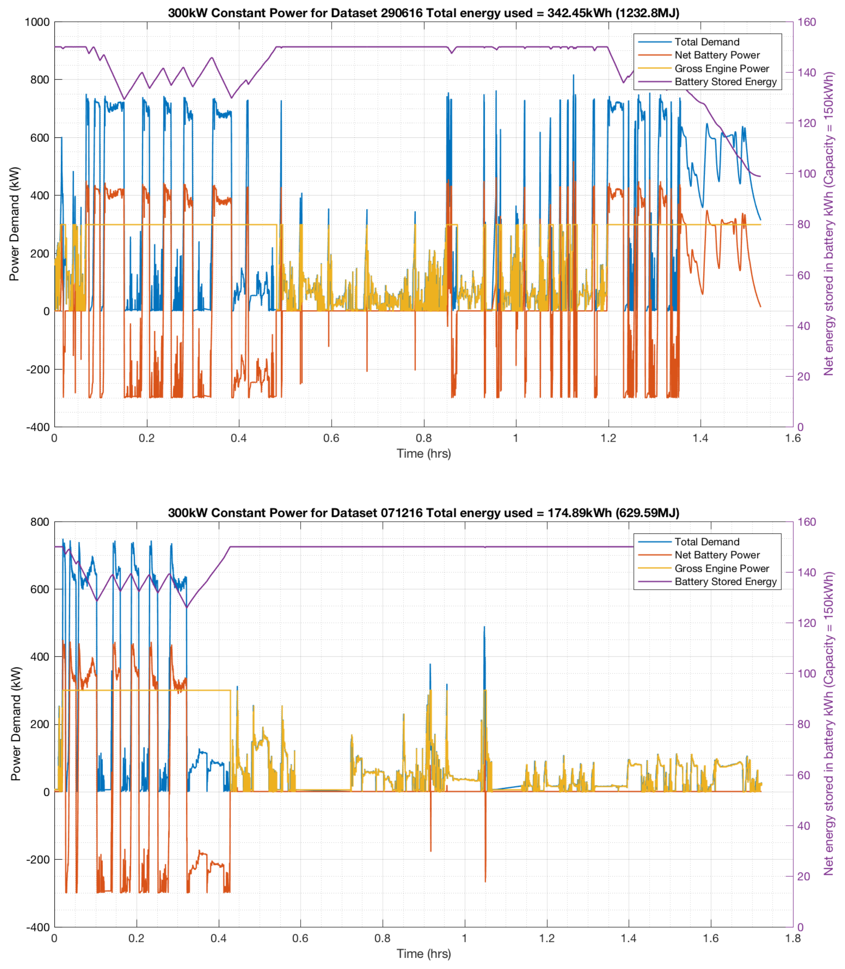
5.6. Full Battery Cycling Scenario

This case requires the engine to frequently provide high power outputs, up to and including full power. This is caused by the restriction of not allowing the battery to switch between charging and discharging states on the fly, meaning that, when the battery is in the charging state, it will spend much of its time inactive due to high power demand values for the vessel, leaving the system with insufficient excess energy available to charge the battery and an engine operating outside its optimal operating envelope.

A positive feature of this system is that the quantification of the battery cycles can be carried out easily because each charging state switch represents a half cycle of the battery (This is based on the assumption that a battery cycle is defined as the battery going full $\to$ empty $\to$ full). The behavior of this regime can be seen by observing the battery state shown in Figure 18.

In this case, the battery capacity was set to 10 kWh merely for illustrative purposes. It can also be seen, by observing the net engine power, that the engine is at times required to provide the full power demand for the system.

5.7. Results

The complexity of the hybrid system poses an increasing amount of design choices for a diesel generator/battery combination. optimizing the operational profile is essential to energy management function design in order to be able to minimize for fuel, emissions, and battery degradation due to micro-cycling.

In this section, we analyze the potential of adding a battery in parallel to the existing diesel engine in order to explore possible fuel savings. The suggested retrofit solution is by no means an efficient solution (i.e., using the existing specification of diesel engine); however, it underlines the benefits and possible cost savings by replacing the existing diesel engine with a completely new hybrid system architecture configuration. The results obtained following the analysis have been captured in

Table 8. Results under a hybrid configuration: Diesel engine 10V 2000 M72 and Battery 1 MWh.

	Diesel Engine Fuel Consumption [L/h]	Hybrid System Fuel Consumption [L/h]	Fuel Consumption Savings [L/h]
First Run (Power Demand of 175 kWh)	187.6	29.6	158
Second Run (Power Demand of 342 kWh)	197	53.3	143.7

.

Our preliminary results demonstrated that we can achieve fuel savings of 70% to 80%. This is because, when power demand is low, for example, during cruising, the diesel engine is operated up to 350 kW, which is the maximum power output to ensure optimal operation. In addition, surplus energy will be stored in the battery if power demand is below 350 kW. When power demand is higher than 350 kW, energy from the battery is utilized. In practice, this power demand would be seen, for example, during docking maneuvers.

5.8. Engine/Battery Pair Matching

It is apparent that the matching of engine power and battery capacity are crucial in the real world scenario. As an example, it was observed that a single run of the vessel (29.06.16) required 343 kWh. This energy is considered to be fundamental as it is a result of the prime moving force of the vessel throughout the run. If there is no plug-in charging for the vessel, then the engine must be sized to $P_{\mathrm{eng}}⩾\overline{P}$. From a practical perspective, it would be suggested that the engine be slightly oversized to allow an operational margin.

From the results of running simulations, the suggestion would be that an engine size of 300 kW and a battery usable capacity of 200 kWh would suffice for the purposes of a functioning hybrid power system for our case. The plotted results from this simulation are shown in Figure 17.

5.9. Challenge and Future Work

Limitations and costs of adding a new hybrid system could relate to retrofitting the hybrid system on “conventional” vessels. Challenges of implementing a hybrid propulsion system to achieve fuel consumption saving could include interoperability, requiring larger amount of batteries than conventional propulsion systems. It remains a question whether and how, on a hybrid vessel, component parts and control systems could be designed to fit the needs of vessel operators [66]. In addition, hybrid system on the vessel could result in large batteries or distributed batteries reducing cargo space. Furthermore, there would be installation costs and potentially further investment required in vessel redesign and customization to accommodate space and weight distributions of batteries.

With respect to future research, areas of investigation that could provide additional optimization to system performance, include:

• Potential for dynamic engine operating set-points. This would allow the engine set-points to be changed by the control system in order to further optimize output emissions.
• Investigation into the potential for use of a multi-regime system. Such a system might change the operation of the hybrid system based on the operation of the vessel, such as having a docking mode which, it might be imagined, could switch the system to run on 100% battery during the docking stages of a journey.
• Data-driven model with more feasibility considerations for live battery prognostic. Currently our battery prognostic model is geared towards outputting live RUL prediction when given dynamic operational data, especially partial charge and discharge data.

6. Conclusions

The marine sector faces global pressure to reduce its CO${}_2$ and NO${}_{\mathrm{x}}$ emissions and increase fuel efficiency, which has led to a surge of interest in the use of hybrid vessels. However, as this work shows, a successful transition of hybrid vessels throughout the marine sector requires an understanding of the operational, environmental, and economic risks and benefits associated with these systems.

The methodology proposed in this paper addresses limitations within the literature that relate to operational prognostics for key assets, system level optimization in energy performance, and integration of environmental, energy demand and asset health key performance indicators. We used a state-of-the-art supervised learning algorithm to predict lithium-ion batteries RUL with relative errors lying under 8.5% for multiple test battery packs, demonstrating the potential for using such algorithm for on-board battery prognostics. We also conducted life cycle tests on a sample of lead-acid batteries as stand-by power sources on a hybrid vessel. The results showed that a clustering machine learning algorithm can achieve an average of 95.5% accuracy in predicting the SOC for lead-acid batteries.

Another key contribution of our work is the design and validation of an autonomous hybrid marine propulsion. Incorporating operational data and automatic multi-objective global optimization for performance (energy), asset health, and environment metrics, we demonstrated that a fuel saving of 70% to 80% can be achieved when using a diesel engine when the energy requirement is below 350 kW, storing surplus energy into battery, and switching to the battery when the energy requirement is above 350 kW.

From our findings, the following recommendations to vessel operators are made: Firstly, it would be valuable to use the internet of things (IoT) to secure operational data on vessel performance; a cost-effective hybrid propulsion system requires a multi-asset optimization architecture, such as the one developed in this paper. Secondly, a cloud platform could add value to the monitoring of hybrid vessel performance trends. Future research will involve determining set-points for dynamic engine operation for emission control, using machine learning algorithms to learn and optimize vessel operations under different stages of a cruise journey, such as docking for automated control decision-making.

References

1. The International Transport Forum. Decarbonising Maritime Transport. 2018. Available online: https://www.itf-oecd.org/sites/default/files/docs/decarbonising-maritime-transport-2035.pdf (accessed on 26 March 2018).
2. Le Quéré, C.; Jackson, R.; Jones, M.; Smith, A.; Abernethy, S.; Andrew, R.; De-Gol, A.; Willis, D.; Shan, Y.; Canadell, J.; et al. Temporary reduction in daily global CO2 emissions during the COVID-19 forced confinement. Nat. Clim. Chang. 2020, 10, 647–653. [Google Scholar] [CrossRef]
3. European Environment Agency. Final Energy Consumption by Mode of Transport. 2017. Available online: https://www.eea.europa.eu/data-and-maps/indicators/transport-final-energy-consumption-by-mode/assessment-8 (accessed on 22 November 2018).
4. United Nations, Development Policy and Analysis Division. World Economic Situation and Prospects. 2012. Available online: http://www.un.org/en/development/desa/policy/wesp (accessed on 11 July 2019).
5. United Kingdom, The Department for Transport. MARITIME 2050, Navigating the Future. 2019. Available online: https://assets.publishing.service.gov.uk/government/uploads/system/uploads (accessed on 16 July 2020).
6. U.S. Energy Information Administration (EIA). International Energy Outlook. 2016. Available online: https://www.eia.gov/outlooks/ieo/pdf/0484(2016).pdf (accessed on 16 July 2020).
7. The Department for Transport, UK. Clean Maritime Plan. 2019. Available online: https://assets.publishing.service.gov.uk/government/uploads/system/uploads/attachment_data/file/815664/clean-maritime-plan.pdf (accessed on 16 July 2020).
8. Geertsma, R.; Negenborn, R.; Visser, K.; Hopman, J. Design and control of hybrid power and propulsion systems for smart ships: A review of developments. Appl. Energy 2017, 194, 30–54. [Google Scholar] [CrossRef]
9. UK Marine Industries Technology Roadmap. 2015. Available online: https://www.maritimeindustries.org/write/Uploads/UKMIA%20Uploads%20-%20DO%20NOT%20DELETE/UK-Marine-Industries-Technology-Roadmap-2015.pdf (accessed on 16 July 2020).
10. Skjong, E.; Volden, R.; Rødskar, E.; Molinas, M.; Johansen, T.A.; Cunningham, J. Past, Present, and Future Challenges of the Marine Vessel’s Electrical Power System. IEEE Trans. Transp. Electrif. 2016, 2, 522–537. [Google Scholar] [CrossRef] [Green Version]
11. Castles, G.; Reed, G.; Bendre, A.; Pitsch, R. Economic benefits of hybrid drive propulsion for naval ships. In Proceedings of the 2009 IEEE Electric Ship Technologies Symposium, Baltimore, MD, USA, 20–22 April 2009; pp. 515–520. [Google Scholar] [CrossRef]
12. EnerSys. Green at Sea: Can the US Navy Cut Its Vast Energy Footprint? 2018. Available online: https://www.naval-technology.com/features/going-green-sea-can-us-navy-cut-vast-energy-footprint/ (accessed on 18 January 2018).
13. Nuhic, A.; Terzimehic, T.; Soczka-Guth, T.; Buchholz, M.; Dietmayer, K. Health diagnosis and remaining useful life prognostics of lithium-ion batteries using data-driven methods. J. Power Sources 2013, 239, 680–688. [Google Scholar] [CrossRef]
14. He, W.; Pecht, M.; Flynn, D.; Dinmohammadi, F. A Physics-Based Electrochemical Model for Lithium-Ion Battery State-of-Charge Estimation Solved by an optimized Projection-Based Method and Moving-Window Filtering. Energies 2018, 11, 2120. [Google Scholar] [CrossRef] [Green Version]
15. Andoni, M.; Tang, W.; Robu, V.; Flynn, D. Data analysis of battery storage systems. CIRED-Open Access Proc. J. 2017, 2017, 96–99. [Google Scholar] [CrossRef] [Green Version]
16. United Kingdom, The Department for Transport. Batteries on Board Ocean-Going Vessels. Available online: https://marine.man-es.com/two-stroke/technical-papers (accessed on 16 July 2020).
17. Frisk, E.; Krysander, M.; Larsson, E. Data-driven lead-acid battery prognostics using random survival forests. In Proceedings of the 2014 Annual Conference of the Prognostics and Health Management Society, Fort Worth, TX, USA, 29 September–2 October 2014; pp. 92–101. [Google Scholar]
18. Solem, S.; Fagerholt, K.; Erikstad, S.; Patricksson, Ø. Optimization of diesel electric machinery system configuration in conceptual ship design. J. Mar. Sci. Technol. 2015, 20, 406–416. [Google Scholar] [CrossRef]
19. Woodyard, D. Exhaust Emissions and Control; Butterworth-Heinemann: Oxford, UK, 2009. [Google Scholar]
20. Flynn, D.; Lofting, D.; Fagogenis, G.; Lane, D.; Record, P.; Herd, D.; Skinn, N. Intelligent asset management for submarines and ships through embedded intelligence. In Proceedings of the Fleet Maintenance & Modernization Symposium (FMMS) 2014, Virginia Beach, VA, USA, 9–10 September 2014. [Google Scholar]
21. Miguelanez-Martin, E.; Flynn, D. Embedded intelligence supporting predictive asset management in the energy sector. In Proceedings of the Asset Management Conference 2015, Washington, DC, USA, 4–5 November 2015; pp. 7–14. [Google Scholar] [CrossRef]
22. Chen, C.; Pecht, M. Prognostics of lithium-ion batteries using model-based and data-driven methods. In Proceedings of the IEEE 2012 Prognostics and System Health Management Conference (PHM-2012 Beijing), Beijing, China, 23–25 May 2012; pp. 1–6. [Google Scholar] [CrossRef]
23. Dong, M.; He, D. Hidden semi-Markov model-based methodology for multi-sensor equipment health diagnosis and prognosis. Eur. J. Oper. Res. 2007, 178, 858–878. [Google Scholar] [CrossRef]
24. Gasperin, M.; Juricic, D.; Boskoski, P.; Vizintin, J. Model-based prognostics of gear health using stochastic dynamical models. Mech. Syst. Signal Process. 2011, 25, 537–548. [Google Scholar] [CrossRef]
25. Tang, W.; Andoni, M.; Robu, V.; Flynn, D. Accurately Forecasting the Health of Energy System Assets. In Proceedings of the International Symposium on Circuits and Systems (ISCAS), Florence, Italy, 27–30 May 2018. [Google Scholar] [CrossRef]
26. Brandsater, A.; Manno, G.; Vanem, E.; Glad, I.K. An application of sensor-based anomaly detection in the maritime industry. In Proceedings of the 2016 IEEE International Conference on Prognostics and Health Management (ICPHM), Ottawa, ON, Canada, 20–22 June 2016; pp. 1–8. [Google Scholar] [CrossRef]
27. Dinmohammadi, F.; Flynn, D.; Bailey, C.; Pecht, M.; Yin, C.; Rajaguru, P.; Robu, V. Predicting Damage and Life Expectancy of Subsea Power Cables in Offshore Renewable Energy Applications. IEEE Access 2019, 7, 54658–54669. [Google Scholar] [CrossRef]
28. Flynn, D.; Tang, W.; Roman, D.; Dickie, R.; Robu, V. Optimization of Hybrid Energy Systems for Maritime Vessels. In Proceedings of the 9th International Conference on Power Electronics, Machines and Drives, Liverpool, UK, 17–18 April 2018. [Google Scholar]
29. Fagogenis, G.; Flynn, D.; Lane, D. Novel RUL prediction of assets based on the integration of auto-regressive models and an RUSBoost classifier. In Proceedings of the 2014 International Conference on Prognostics and Health Management, Fort Worth, TX, USA, 29 September–2 October 2014; pp. 1–6. [Google Scholar]
30. Kirschbaum, L.; Dinmohammadi, F.; Flynn, D.; Robu, V.; Pecht, M. Failure Analysis Informing Embedded Health Monitoring of Electromagnetic Relays. In Proceedings of the 2018 3rd International Conference on System Reliability and Safety (ICSRS), Barcelona, Spain, 23–25 November 2018; pp. 261–267. [Google Scholar] [CrossRef]
31. Turner, S. Russian roulette: Loading the barrel with statistics and pulling the trigger on reliability. In Proceedings of the Asset Management Conference, Sydney, Australia, 1–5 June 2009. [Google Scholar]
32. Roman, D.; Dickie, R.; Flynn, D.; Robu, V. A Review of the Role of Prognostics in Predicting the Remaining Useful Life of Assets. In Proceedings of the 27th European Safety and Reliability Conference, Portoroz, Slovenia, 18–22 June 2017. [Google Scholar]
33. Pecht, M.G. Prognostics and Health Management of Electronics; Wiley: Hoboken, NJ, USA, 2008. [Google Scholar]
34. Pecht, M.G.; Kang, M. PHM of Subsea Cables. In Prognostics and Health Management of Electronics: Fundamentals, Machine Learning, and the Internet of Things; Wiley: Hoboken, NJ, USA, 2019; pp. 451–478. [Google Scholar]
35. Kumar, S.; Pecht, M. Modeling Approaches for Prognostics and Health Management of Electronics. Int. J. Perform. Eng. 2010, 6, 467–476. [Google Scholar]
36. Kirschbaum, L.; Roman, D.; Singh, G.; Bruns, J.; Robu, V.; Flynn, D. AI-driven Maintenance Support for Downhole Tools and Electronics Operated in Dynamic Drilling Environments. IEEE Access 2020, 8, 78683–78701. [Google Scholar] [CrossRef]
37. Pecht, M.; Jaai, R. A prognostics and health management roadmap for information and electronics-rich systems. Microelectron. Reliab. 2010, 50, 317–323. [Google Scholar] [CrossRef]
38. Michau, G.; Palmé, T.; Fink, O. Fleet PHM for Critical Systems: Bi-level Deep Learning Approach for Fault Detection. In Proceedings of the European Conference of the PHM Society, Philadelphia, PA, USA, 24–27 September 2018; pp. 401–407. [Google Scholar]
39. Kanellos, F.D. Optimal Power Management with GHG Emissions Limitation in All-Electric Ship Power Systems Comprising Energy Storage Systems. IEEE Trans. Power Syst. 2014, 29, 330–339. [Google Scholar] [CrossRef]
40. Shang, C.; Srinivasan, D.; Reindl, T. Economic and Environmental Generation and Voyage Scheduling of All-Electric Ships. IEEE Trans. Power Syst. 2016, 31, 4087–4096. [Google Scholar] [CrossRef]
41. Kanellos, F.D.; Prousalidis, J.M.; Tsekouras, G.J. Control system for fuel consumption minimization as emission limitation of full electric propulsion ship power systems. Proc. Inst. Mech. Eng. Part M J. Eng. Marit. Environ. 2014, 228, 17–28. [Google Scholar] [CrossRef]
42. Grimmelius, H.; de Vos, P.; Krijgsman, M.; van Deursen, E. Control of Hybrid Ship Drive Systems. In Proceedings of the 10th International Conference on Computer and IT Applications in the Maritime Industries, Hamburg, Germany, 2–4 May 2011; pp. 1–14. [Google Scholar]
43. Vu, T.L.; Ayu, A.A.; Dhupia, J.S.; Kennedy, L.; Adnanes, A.K. Power Management for Electric Tugboats Through Operating Load Estimation. IEEE Trans. Control Syst. Technol. 2015, 23, 2375–2382. [Google Scholar] [CrossRef]
44. Caledonian Maritime Assets Ltd. The Hybrid Ferries Project. Available online: http://www.cmassets.co.uk/project/hybrid-ferries-project (accessed on 16 July 2020).
45. Sciberras, E.A.; Norman, R.A. Multi-objective design of a hybrid propulsion system for marine vessels. IET Electr. Syst. Transp. 2012, 2, 148–157. [Google Scholar] [CrossRef]
46. Dimas, D.; Katsikas, S.; Defigos, A.; Routzomanis, A.; Mermikli, K. Wireless Modular System for Vessel Engines Monitoring, Condition Based Maintenance and Vessell’s Performance Analysis. In Proceedings of the 2nd European Conference of the Prognostics and Health Management Society, Nantes, France, 24–27 July 2014; Volume 5. [Google Scholar]
47. The Swedish Club. Main Engine Damage. Available online: https://www.swedishclub.com/ (accessed on 16 July 2020).
48. Niculita, O.; Nwora, O.; Skaf, Z. Towards Design of Prognostics and Health Management Solutions for Maritime Assets. In Proceedings of the 5th International Conference in Through-Life Engineering Services, Cranfield, UK, 1–2 November 2016; pp. 122–132. [Google Scholar] [CrossRef]
49. Tipping, M.E. Sparse Bayesian learning and the relevance vector machine. J. Mach. Learn. Res. 2001, 1, 211–244. [Google Scholar]
50. Hearst, M.A.; Dumais, S.T.; Osman, E.; Platt, J.; Scholkopf, B. Support vector machines. IEEE Intell. Syst. Appl. 1998, 13, 18–28. [Google Scholar] [CrossRef] [Green Version]
51. Tipping, M.; Faul, A. Fast Marginal Likelihood Maximisation for Sparse Bayesian Models. In Proceedings of the 9th International Workshop on Artificial Intelligence and Statistics, Key West, FL, USA, 3–6 January 2003. [Google Scholar]
52. Dempster, A.P.; Laird, N.M.; Rubin, D.B. Maximum likelihood from incomplete data via the EM algorithm. J. R. Stat. Soc. Ser. B 1977, 39, 1–38. [Google Scholar]
53. Saha, B.; Goebel, K. Battery Data Set. National Aeronautics and Space Administration (NASA) Ames Prognostics Data Repository. 2007. Available online: https://ti.arc.nasa.gov/tech/dash/groups/pcoe/prognostic-data-repository/ (accessed on 16 July 2020).
54. Liu, D.; Wang, H.; Peng, Y.; Xie, W.; Liao, H. Satellite Lithium-Ion Battery Remaining Cycle Life Prediction with Novel Indirect Health Indicator Extraction. Energies 2013, 6, 3654–3668. [Google Scholar] [CrossRef]
55. Eddahech, A.; Briat, O.; Vinassa, J.M. Determination of lithium-ion battery state-of-health based on constant-voltage charge phase. J. Power Sources 2014, 258, 218–227. [Google Scholar] [CrossRef]
56. Hu, C.; Jain, G.; Zhang, P.; Schmidt, C.; Gomadam, P.; Gorka, T. Data-driven method based on particle swarm optimization and k-nearest neighbor regression for estimating capacity of lithium-ion battery. Appl. Energy 2014, 129, 49–55. [Google Scholar] [CrossRef]
57. Ma, S.; Jiang, M.; Tao, P.; Song, C.; Wu, J.; Wang, J.; Deng, T.; Shang, W. Temperature effect and thermal impact in lithium-ion batteries: A review. Prog. Nat. Sci. Mater. Int. 2018, 28, 653–666. [Google Scholar] [CrossRef]
58. Onda, K.; Ohshima, T.; Nakayama, M.; Fukuda, K.; Araki, T. Thermal behavior of small lithium-ion battery during rapid charge and discharge cycles. J. Power Sources 2006, 158, 535–542. [Google Scholar] [CrossRef]
59. EnerSys. Ohmic Measurements as a Maintenance Tool for Lead Acid Stationary Cells. Available online: http://www.newark.com/pdfs/techarticles/enersys (accessed on 16 July 2020).
60. Duda, R.O.; Hart, P.E.; Stork, D.G. Pattern Classification, 2nd ed.; Wiley-Interscience: Hoboken, NJ, USA, 2000. [Google Scholar]
61. Coraddu, A.; Oneto, L.; Baldi, F.; Anguita, D. Vessels Fuel Consumption: A Data Analytics Perspective to Sustainability. In Soft Computing for Sustainability Science; Cruz Corona, C., Ed.; Springer International Publishing: Cham, Switzerland, 2018; pp. 11–48. [Google Scholar] [CrossRef]
62. Harris, H. Prediction of the torque and optimum operating point of diesel engines using engine speed and fuel consumption. J. Agric. Eng. Res. 1992, 53, 93–101. [Google Scholar] [CrossRef]
63. Trodden, D.G.; Murphy, A.P.K. Evaluation of Emission Factors on the Estimation of NOx Formation from a Manoeuvring Ship. Transp. Res. Part D Transp. Environ. 2010, 15, 204–221. [Google Scholar] [CrossRef]
64. Wang, G.; Zoerb, G. Determination of optimum working points for diesel engines. Trans. ASAE 1989, 32, 1519–1522. [Google Scholar] [CrossRef]
65. Lin, C.C.; Peng, H.; Grizzle, J.W.; Kang, J.M. Power management strategy for a parallel hybrid electric truck. IEEE Trans. Control Syst. Technol. 2003, 11, 839–849. [Google Scholar] [CrossRef] [Green Version]
66. Newman, N. Hybrid Ships Take to the High Seas. Available online: https://eandt.theiet.org/content/articles/2019/01/hybrid-ships-take-to-the-high-seas (accessed on 17 January 2019).
Figure 1. Overall system architecture and workflow.
Energies 13 04676 g001
Figure 2. Cyclone clipper, drawings, and dimensions.
Energies 13 04676 g002
Figure 3. Workflow of the remaining useful life (RUL) estimation model.
Energies 13 04676 g003
Figure 4. RUL loss curve for battery No. 5.
Energies 13 04676 g004
Figure 5. DC pulse test.
Energies 13 04676 g005
Figure 6. Lead-acid test system.
Energies 13 04676 g006
Figure 7. Engine fuel consumption function.
Energies 13 04676 g007
Figure 8. Fuel contour map (g/kWh).
Energies 13 04676 g008
Figure 9. Nitrogen oxide (NOx) emissions compared against power and torque.
Energies 13 04676 g009
Figure 10. NOx emissions against power and exhaust temperature.
Energies 13 04676 g010
Figure 11. NOx emissions compared against power and temperature.
Energies 13 04676 g011
Figure 12. MTU 10V 2000 M72 diesel engine-specific NOx emissions contour map.
Energies 13 04676 g012
Figure 13. Decision flow chart for the battery algorithm.
Energies 13 04676 g013
Figure 14. Power demand histogram for 29.06.16 and 07.12.16 datasets.
Energies 13 04676 g014
Figure 15. Plot of demand for 29.06.16 and 07.12.16 datasets.
Energies 13 04676 g015
Figure 16. Energy state of an 800 kWh battery for 29.06.16 and 07.12.16 datasets using battery only.
Energies 13 04676 g016
Figure 17. Simulation results for engine setpoint of 300 kW and battery capacity of 150 kWh.
Energies 13 04676 g017
Figure 18. Battery operation under full cycle restriction.
Energies 13 04676 g018