Nonlinear Optimization of Turbine Conjugate Heat Transfer with Iterative Machine Learning and Training Sample Replacement

Abstract

A simple yet effective optimization technique is developed to solve nonlinear conjugate heat transfer. The proposed Nonlinear Optimization with Replacement Strategy (NORS) is a mutation of several existing optimization processes. With the improvements of 3D metal printing of turbine components, it is feasible to have film holes with unconventional diameters, as these holes are created while printing the component. This paper seeks to optimize each film hole diameter at the leading edge of a turbine vane to satisfy several optimum thermal design objectives with given design constraints. The design technique developed uses linear regression-based machine learning model and further optimizes with strategic improvement of the training dataset. Optimization needs cost and benefit criteria are used to base its decision of success, and cost is minimized with maximum benefit within given constraints. This study minimizes the coolant flow (cost) while satisfying the constraints on average metal temperature and metal temperature variations (benefits) that limit the useful life of turbine components. The proposed NORS methodology provides a scientific basis for selecting design parameters in a nonlinear design space. This model is also a potential academic tool to be used in thesis works without demanding extensive computing resources.

1. Introduction

The inspiration for this work came from the existing need to find the optimum film hole diameter with available correlations on flow and heat transfer. However, it soon became apparent that a new optimization technique has been developed that is simple and yet effective. Without getting into too many mathematical formulations, the proposed Nonlinear Optimization with Replacement Strategy (NORS) can use existing optimization routines and switch between model-based and model-free machine learning domains to get a better design than what could be obtained with random selection of design parameters. The procedure is simple, does not require significant computing power, routines are available as open access, and it can be applied in any engineering or financial analysis, where the input and output have established correlations available. In the past decade, significant proportion of thermal sciences masters’ students used nanofluid to graduate and some of the project topics on that were listed by Saidur et al. (2011) [1]. Increase in thermal conductivity by adding nanoparticles in fluids is an interesting concept, has a catchy name, and easy to implement in labs. The process: take some nanopowder, mix with water or other fluid, and run convective heat transfer experiments. Thousands of students effectively used this route to satisfy their graduation requirements, but it is somewhat getting overused and could not find as much industrial use as it hoped for. There is a need for a new path, and this NORS-based research presents a new opportunity to give graduate students a taste for both model-based and model-free machine learning techniques with artificial intelligence. NORS has endless optimization combination opportunities and will provide several years of academic optimization education and industrial competitive design improvements. NORS does not spend too much effort to find the absolute best design, rather it improves on the engineering design from the given trend or given set of observations. It is effective, flexible, and yet not computationally expensive. All the work done here was accomplished on a regular college student’s laptop, making it attractive for graduate students and university faculties.

The proposed work develops an optimization technique based on numerical simulations and model learning. The example selected is a conjugate thermal model where both convection and conduction play major roles to provide temperature distribution, which has design constraints. In gas turbine heat transfer analysis, nonlinear influences of diverse set of parameters are present simultaneously and they interact with each other, making an optimized solution very hard to achieve. Proposed optimization involves complicated cooling technologies with impingement, developing flow in film holes, pressure drop in the film hole, external gas flow conditions, and the showerhead film effectiveness on the external face. Selected design parameters are implemented through an ANSYS-based finite element (FE) model and a Python-based optimization scheme. Learning mode FE outputs were processed with linear regression, and those machine-learned models were used for thermal optimization. A convex optimization technique is adopted to minimize coolant flowrate by varying film hole diameters. The constraints on optimization were on the size of the film holes, average metal temperature, and temperature variation among different regions of the component.

This work is an attempt to apply optimization techniques available in engineering for turbine cooling performance improvement. Optimization has become relevant in recent developments due to the availability of additive manufacturing and the possibility to get into uneven complicated shapes that were nearly impossible to build and impractical to implement only a few years ago. Additive manufacturing made it feasible to design optimized conduction paths with unique conductor shapes to maximize heat transfer with minimum size. Menge et al. [2] showed a tree-like structure to conduct heat away from electronic heat source from a projector assembly. Due to proprietary technology, they did not provide the mathematical scheme used to gain improved cooling with an innovative tree root-like conductive structure that optimized mass and improved cooling by carrying the heat away from the source to the sink. In this work, we have numerically experimented to implement an optimization routine that does not demand heavy computation efforts and the results are encouraging. Most of the correlations used in our paper are taken from Han et al. [3], and we have kept our formulation flexible so that any other correlation can be used to optimize other thermal designs as needed. To separate the correlations from optimization, a model-free routine is developed. Governing equations and model details for flow are provided in Dutta and Smith [4].

Several publications discussed improvements in design with conjugate heat transfer (CHT). Notably Prof. Thole’s group at the Penn State, Prof. Han’s laboratory at Texas A&M Univ., and Prof. Bogard’s group at the Univ. of Texas at Austin have done a wide variety of research on gas turbines that we have referenced while developing our model [4]. Jennings [5] summarized those CHT works till 2011 and showed that CHT was very important while tuning the film cooling in gas turbine applications. The design of gas turbine blades and vanes is a challenging task. The nature of the problem calls for high speed flow in extreme conditions, high temperature and pressure with significant gradients, and turbulent flows with moving parts to be predicted accurately. The conventional technique for solving such flows neglected conduction through the blade material and relied on turbulence models to predict the film-cooled flow. However, predicted results with improper conjugate analysis found to have errors as large as 14% when predicting the wall temperature for internally cooled turbine airfoils. Designers are aiming for tighter tolerances than that and therefore CHT studies are getting attention. The CHT techniques are computationally expensive and experiments needed to understand them are challenging as the heat flow gets more complicated. Instead of searching for an optimum configuration by trial and error, our paper provides guidelines to develop a systematic technique towards an optimized solution that would have taken significant time and investment to achieve otherwise.

The efficient gas turbines of today require both internal and external modes of airfoil cooling for the survival of airfoils in extremely harsh conditions (Town et al. [6]). Only one mode of cooling could not sustain the thermal load effectively. Cooling designs have evolved from simple internal convective channels to double-wall configurations and advanced shaped film-holes. Their paper described the development of airfoil’s inner and outer cooling designs. Presented cooling concepts were based on a summary of peer reviewed publications, patents, and feedbacks from academia and industry. Like present analysis, the leading edge was internally cooled by jet impingement on the inner surface and externally protected with showerhead film cooling. The mid-region of the airfoil had a three-pass serpentine passage with internal V-shaped ribs to increase the channel heat transfer coefficient. There were multiple rows of shaped diffusion holes in this mid-region. The trailing edge was cooled with jet impingement on the inside and pressure side gill-slot film. Even though our work only addresses the leading-edge cooling optimization, the proposed NORS technique can be used to optimize the entire airfoil or some other subsection of the component.

Carnot cycle efficiency suggests higher inlet temperature in turbine improves thermal efficiency. The continuing rise in turbine entry temperatures, also known as firing temperature, to have better thermal efficiency require continued innovations in the cooling technology as many researchers have illustrated in annual ASME Turbo Expo over the past decades. Most of the time, knowledge learnt from one setting could not be scaled for other operating situations or a simple addition of effects did not work. Murray et al. [7] discussed effusion cooling as an example of stitching together multiple smaller film holes. It was characterized by a high density of smaller diameter film cooling holes operating at low blowing ratios with higher overall cooling effectiveness. They evaluated effusion system’s cooling performance with both experimental and computational analyses. Two flat-plate geometries were experimentally investigated with a high surface resolution pressure sensitive paint technique. Pressure sensitive paints use a heat-mass transfer analogy and provide detail two-dimensional film effectiveness distribution. A computational fluid dynamics (CFD) scalar tracking method was used to model the experimental setup. Computational predictions compared favorably with experimental observations. The CFD domain was simplified to assess the cooling performance from a single film hole ejection. A superposition method was developed and applied to the resulting two-dimensional film effectiveness distribution that shortened the time needed to obtain thermal conditions for an array of dense holes. A faster analysis of a multi-hole effusion type setup was achieved and the technique produced acceptable results at larger hole spacings; however, with denser holes, the predictions were not as good. It was argued that high levels of jet interactions reduced the performance of the superposition method. This indicates there is always a risk in using data from a different set of hole configuration, but there is a gain in prediction time and therefore benefits need to be scaled with the possible risks to get a meaningful outcome.

Even if our primary objective is to build an efficient optimization process for the nonlinear engineering domain, the application selected is to optimize a three-dimensional temperature distribution in a gas turbine component. To explain three-dimensional temperature predictions, Hwang et al. [8] used ANSYS CFX V16.0 to study conjugate heat transfer on a turbine blade with both steady and unsteady effects. The first stage high pressure turbine experimental data from 1983 NASA internally cooled C3X was used to validate the conjugate numerical heat transfer. Results from the unsteady state were compared to the results of steady state calculations, and they observed that unsteady conjugate heat transfer analysis of the rotor blade was important for cooling design process. Their prediction of the thermal environment around the rotor blade and heat conduction analysis provided confidence with the numerical thermal load analysis.

Jennings [5] developed a loosely coupled conjugate heat transfer method called Iterative Conjugate Heat Transfer (ICHT) to incorporate conjugate effects in film-cooled components. A Reduced-Order Film Model (ROFM) was also developed to use experimental data or empirical correlations in place of turbulence models for solving film-cooled flow. ROFM automated the process of setting up and solving CFD solutions. The development and a demonstration of this technique included a CFD solution of a film cooled C3X blade. The influence of conjugate effects and the accuracy of ROFM were estimated. Results showed a maximum deviation for wall temperatures of 3.33%, which was ~2.5% of the initial total gas temperature, and equivalent to 18 °C, showing good agreement with experimental results. The change in wall temperature due to conjugate effects in comparison to non-conjugate studies was a maximum of 40 °C, which is considered very significant in gas turbine design. Kistenmacher [9] experimentally studied the effects of film cooling and thermal barrier coating on gas turbine vane with conjugate heat transfer. That work tried to develop an analytical model to correlate experimental observations with limited success, showing the complexities in these conjugate energy transfers. Williams et al. [10] illustrated the importance of internal cooling and studied the impact of impingement with and without film cooling to validate the need for internal impingement. They concluded that both internal and external cooling were needed to achieve better cooling efficiency.

There are significant amounts of mathematical and statistical techniques involved in any optimization problem. Notably, Ghobadi [11] has discussed mathematical aspects of transient heat conduction optimization. That work was good but unfortunately was not published in peer-reviewed journal or conference. Another example of an optimization problem that included integral and partial differential equation constraints for a heat transfer optimization problem was discussed by Betts and Campbell [12]. To make optimal control methods applicable for a thermal problem, they carefully chose the objective functions and the constraints. Their first step to solve the problem was to discretize the functions in space. Then, Hamiltonian systems and adjoint variables, as described by Betts [13], were used to derive the optimality conditions. Optimization was solved with Sparse Optimal Control Software (SOCS) (explained in Betts and Huffman) [14]. This approach was called “optimize then discretize”. As they observed, this method had difficulty to converge for even very small number of discretization points. They suggested that the “discretize then optimize” approach would work much better for heat transfer. The “discretized then optimize” methodology for the Betts–Campbell heat transfer optimization problem is elaborated more in [11]. These optimization studies focused on changing boundary conditions to get desired results in a given geometry. Our work modifies the geometry to adapt to given boundary conditions for optimal energy usage. The analysis domain was found to be convex in nature for optimization.

A problem needs to be converted to a standard form of linear equations or needs a custom solver to be analyzed with convex optimization techniques. These tasks are time consuming and the intermediate steps can introduce new errors in calculations. DSL—a domain specific language, allows the user to implement specific commands for specialized tasks. SQL, HTML, and CSS are examples of DSL. There are special DSLs developed for convex optimization and some of the examples are: CVX (Grant and Boyd), YALMIP (Lofberg), QCML (Chu et al.), PICOS (Sagnol), and Convex.jl (Udell et al.) [15,16,17,18,19]. Instead of developing a new solver, we have converted our governing equations in linearized optimization routines as explained in the paper. Convex optimization technique has many applications to fields as diverse as machine learning, control, finance, signal and image processing (Diamond and Boyd [20]; Boyd and Vandenberghe [21]). We are adding thermal sciences to this growing list. The optimization for this CHT analysis was performed using the SciPy optimization function “minimize” and the constrained minimization solver was SLSQP, or Sequential Least SQuares Programming [22]. This routine worked better with the given scenarios. More discussion on optimization routines is provided by Carlberg [23].

The organization of the paper is laid out as an introduction to basic concepts, conjugate heat transfer configuration, model development, boundary conditions, optimization and iteration methods, results, and discussion, followed by conclusions.

2. Conjugate Heat Transfer Configuration

There are many experimental measurements and numerical predictions available in published literature to understand film cooling and jet impingement flow, as well as the related heat transfer. There are studies to understand them as independent cooling techniques in addition to studies to tie them together as conjugate heat transfer [24]. In this work, we have developed a technique with linear regression and design of experiments to improve the conjugate heat transfer in a leading edge of a gas turbine airfoil. The objective of the present work is to develop a technique that is computationally economical but provides systematic optimum results (rather than a trial and error method) on a balanced objective with acceptable results. The cooling configuration selected for the optimization process is the leading edge of an airfoil with internal impingement cooling and external film cooling. The geometry modeled is a hollow half-cylinder on which rows of film holes are straight drilled. This type of film hole arrangement is also known as shower head arrangement. The diameter of each film hole is varied to get an optimized heat transfer solution that minimizes on the coolant flow and keeps the metal temperature within operating limits.

A transfer function approach (essentially, a linear regression for our work) is widely used in the industry to capture the effects of multiple parameters on a target result. According to Wikipedia and the electrical engineering-based definition [25,26], “A transfer function of an electronic or control system component is a mathematical function, which theoretically models the device’s output.” The model developed here uses hole diameters as input, and the amount of coolant flow and associated temperature distribution as output. The performance of cooling is defined by rules related to the temperature distribution, which are implemented as constraints of the model. More definitions related to transfer function are available in [27,28,29]. In a simple one input-one output configuration, a transfer function is an equation or plot defining dependent outputs with given independent inputs. The curve is called a transfer curve or characteristic curve. However, for our work there are multiple parameters and multiple curves to optimize with complicated constraints and nonlinear relationships among cost and investment performance functions.

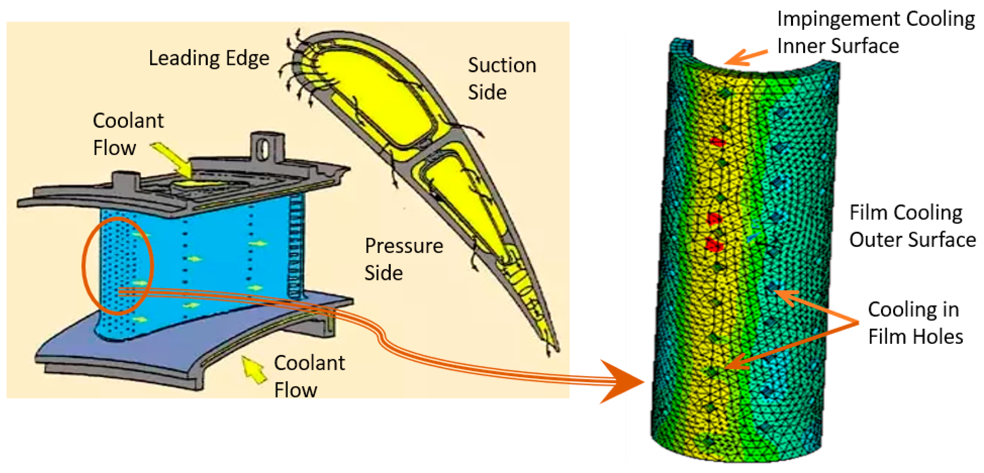
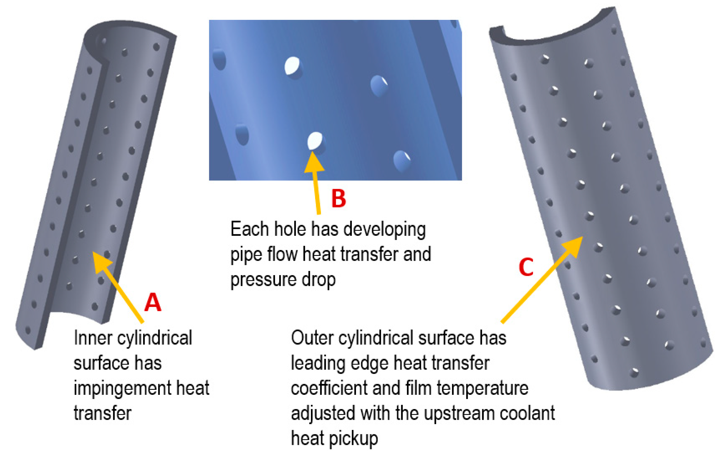
The physical model used for analysis, in addition to the corresponding location in a gas turbine vane, is illustrated in Figure 1. As this work seeks to provide a scientific methodology for optimization of film holes rather than focusing on the accuracy of the expressed temperatures in a real component, a half-cylinder sufficiently approximates the leading edge of a gas turbine vane. To model the heat transfer characteristics within the vane, the boundary conditions include internal impingement, thermally and hydrodynamically developing flow in film holes, and external film cooling. The conduction within the vane is provided through the finite element software to provide a conjugate heat transfer analysis for the leading edge of the vane. The FE solver used here is ANSYS Mechanical APDL 19.0. The scope of this work is limited to finding optimum hole sizes on given film locations. There are other optimizations possible but could not be addressed due to additional complexities like hole locations and adjustment in number of holes. The model accuracy and robustness were verified with local 1D heat balance at selected spots, and boundary conditions were flexed in both plus and minus directions and results were observed to be sensible.

There were a few thermal optimizations done on turbine components, notably Grzegorz and Wlodzimierz [30] optimized the internal cooling schemes in an airfoil with external boundary conditions as given and fixed. Unlike their work, in our study, both the external and internal boundary conditions were affected by the optimization of film hole diameters that metered the coolant flow. Wang et al. [31] used neural and genetic algorithms to optimize film hole shape. Nowak et al. [30] optimized the interior structures of a steam turbine airfoil and found that it was computationally demanding. Our proposed NORS optimization technique is simple and yet proved to be effective for thermal optimization. All the presented work was done in laptops. To extend the work on a bigger component will require a workstation, but perhaps no supercomputing effort is needed.

Fluid Flow through Film Holes

As the coolant flow is driven by a pressure drop from pre-impingement (source) to the external flow (dump), the governing equation for flow can be modeled using standard flow equations with losses. Available fluid flow equations use discharge coefficients for the impingement holes and the viscous loss coefficient for film holes as calculated from friction factor [4]. As the friction factor is a function of flow velocity, hole size, and resulting Reynolds number, the friction factor and hole size are interdependent. To calculate these values, an initial approximation was taken from Moody’s friction factor chart [33], and then velocity and friction factor were calculated iteratively.

As film hole diameters are the knobs for adjusting in this cooling performance, each hole is treated separately for flow balance and heat pickup by coolant. The external film is strongly dependent on the local exit coolant temperature of the film and the film effectiveness value is dependent on the flow velocity and hole size. Therefore, each hole contributed independently on all three zones, internal impingement, convection in hole, and external film parameters. To incorporate film effectiveness at each film hole into the model, the coolant exit temperature was used to determine the external boundary conditions of the numerical model.

3. Model Development

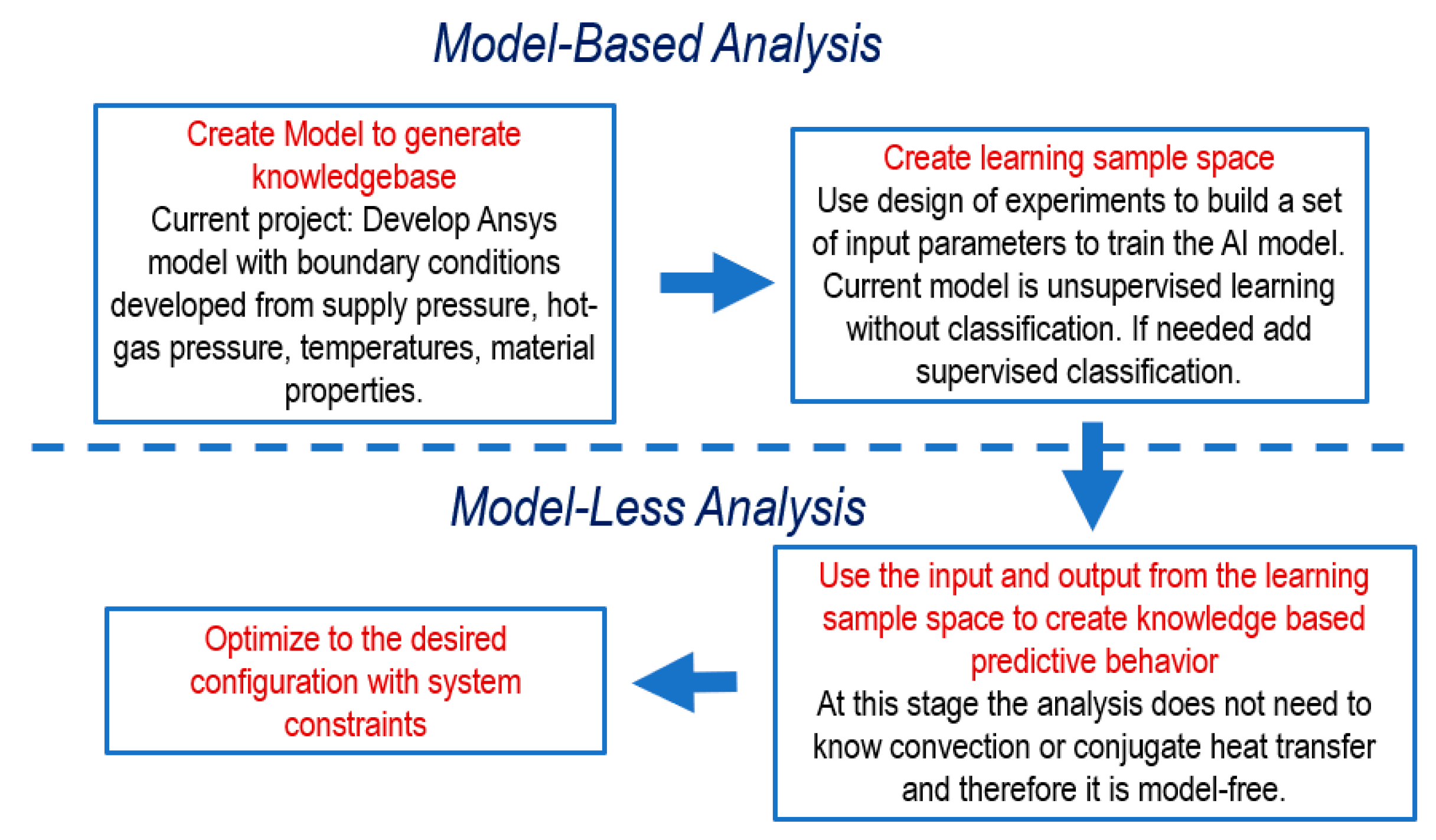
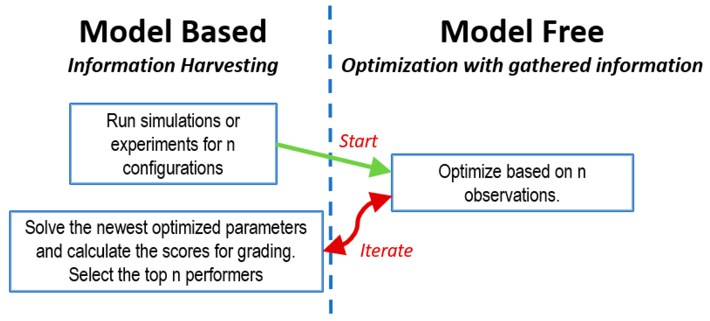
Figure 2 shows the overall process of formulation and optimization. The user needs to identify the given inputs like hot-gas temperature and heat transfer coefficient profiles, coolant supply pressure and temperature, hot-gas pressure, and temperature. The coolant flow is established by the pressure difference between the pre-impingement supply and outer dump pressures, and this pressure difference usually remains constant during the turbine full-load operation. The proposed optimization routine uses constraints on hole diameter size, allowable maximum metal temperature, and limits on metal temperature spatial fluctuations. The objective of the optimization task is to minimize coolant flow while satisfying the constraints.

Fortunately, the variations in coolant flow rate with changing diameter are a convex function, which helps significantly with the optimization process. However, the constraints impose restrictions, and interactions of neighboring holes make detailed equations complicated. Results indicate that the optimized result is better than the initial guess as obtained with DOE analysis. The temperature fluctuations caused by neighboring film holes are harder to understand and the transfer function approach provided a simple but effective way to predict the complicated conjugate heat transfer with reasonable outcome.

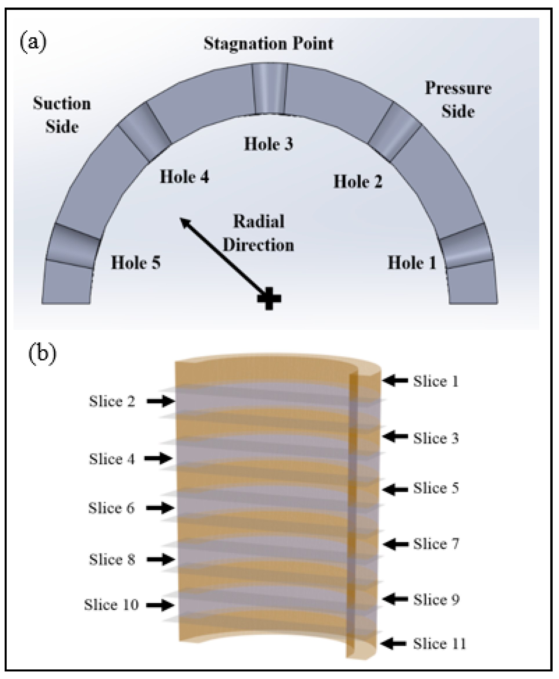
The leading edge vane model contains 53 film holes, while the half-cylinder has an inner radius of 15 mm and a thickness of 4 mm. As shown in Figure 3, the model contains 5 film hole columns, with the columns 1, 3, and 5 having 11 film holes each, while columns 2 and 4 have 10 film holes. FE model is discretized with tet-mesh with 15,416 elements and 28,858 nodes, with the mesh containing three equal layers in the cylinder’s radial direction. For simplicity, the model contains a constant thermal conductivity of 15 W/mK reflecting the properties of Inconel, a high temperature alloy.

For analysis and optimization of the model, the leading edge was broken into 11 slices, corresponding to a 10 mm zone of the 110 mm long model (Figure 3b). The external boundary conditions were broken into five zones in each slice, with each zone centered around a film hole. This essentially provided the individual effect of film hole size on the film temperature.

Regression for Optimization

The optimization routine sets the objective as minimizing total coolant flowrate. To build the temperature constraint from nearly 29,000 nodes required creating a transfer function with linear regression from FE results. This transfer function used diameter of each hole as input and the average nodal temperature within the selected slice as output to determine the associated coefficients for each hole and experimental run. Coefficients ‘a’ in Equation (1) serve as placeholders for the dataset development, but calculating their value is not necessary for creating the transfer function.

$$\begin{gathered} a_1{d}_{11}+\dots +a_n{d}_{1n}=T_{avg,1} \\ \dots \\ {a}_1{d}_{m1}+\dots +a_n{d}_{mn}=T_{avg,m} \end{gathered}$$

(1)

Equation (1) describes the dataset used for transfer function development, created in a Python Pandas dataframe, for which m is the training dataset number and n is the hole number. There are a-coefficients for each hole and a set of diameters for each training data combination. A dataset was created for each slice, resulting in 11 datasets, each containing results for the 13 training datasets of that iteration. The regression uses the dataset for each slice to provide a single equation which predicts the slice temperature as a function of hole diameters. Once the regression is run for each slice, the overall vane temperature can be predicted by the transfer function. This function is created by compiling the set of regression equations which predict the temperature of each slice as a function of the inputted diameters. The linear regressions consistently had R² values over 0.98, indicating that the linear regression was sufficient for modeling the transfer function. Equation (2) shows the format of transfer functions used for this work.

$$\begin{gathered} b_1{d}_1+b_2{d}_2+b_3{d}_3+b_4{d}_4+b_5{d}_5=T_{slice,1} \\ \dots \\ {b}_{51}{d}_{51}+b_{52}{d}_{52}+b_{53}{d}_{53}=T_{slice,11} \end{gathered}$$

(2)

As Equation (2) describes the transfer function for all holes using the transfer function coefficients ‘b’, the optimization routine can predict vane temperature and the temperature of each slice reasonably well. There is some effect from one slice to the other, but adding those effects are computationally expensive. The objective of this work is not about finding the exact solution but an adequate outcome with reasonable effort. For this paper, a desired metal temperature of 1003 K was selected, as it was the average of the temperatures which fit in the bounds of the regression equations for each slice on the initial set of DOE diameters. As a reminder, this study seeks to demonstrate a methodology for iterative film hole optimization, rather than focusing on whether this desired temperature is what should be selected by those in industry.

The optimization is performed using the SciPy optimization function named “minimize” and the constrained minimization solver SLSQP (Sequential Least SQuares Programming). The optimization routine uses an objective function of coolant flowrate, while the constraining function required that predicted slice average temperatures were under the desired temperature, which in this case is set to 1003 K. Optimizing each slice to fit the desired temperature profile allows for the entire vane to be tailored to the desired temperature and reduces the standard deviation in temperatures between slices. Once the set of optimized diameters was obtained, that newly optimized set replaced the set of diameters with lowest performance grade, and the iterative process continued. There is no hard stopping point for this, as the desired standard deviation can be lowered to get better result till a divergence is observed. While the original DOE used whole values of 2, 3, or 4 mm film holes, fractions of millimeters were permitted for the optimized diameters. This assumes that with advances in additive manufacturing, this level of precision is possible for film hole construction while printing the component.

4. Boundary Conditions

4.1. Leading Edge Boundary Conditions

The leading edge boundary conditions were developed through the use of an average Nusselt number for the stagnation region and a profile provided by Mehendale et al. (1991) [34] in combination with a Nusselt percentage multiplier in the chord distance along pressure side and suction side of a typical airfoil. The net results are shown in Figure 4. The Nusselt number provided the h, and the hot-gas temperature was taken from the imposed profile by the mainstream hot-gas in combination of film coolant coming out of the shower head film holes. The film effectiveness correlation is taken from Han et al. (2012) [3]. A summary of boundary conditions is listed in

Table 1. Boundary conditions applied on the numerical half cylinder model with film holes.

Surface	Boundary Condition
Top, Bottom, and Sides	Insulated, assuming symmetry
Inner Cylinder Surface	Jet impingement array [35]
Outer Cylinder Surface	Flow over an airfoil superimposed with film effectiveness based on film configuration and exit temperature from film hole [34]
Inside of Film Hole	Developing turbulent flow in a pipe with entry temperature as post-impingement [36]

.

These boundary conditions are taken from established experimental measurements. More complex real engine conditions use proprietary information, but the design engineer can use any recommended correlation without disturbing the underlying optimization technique proposed here as the technique is divided in two parts—one is model-dependent where the correlations play a role, and the other part is model-free, where no knowledge of film cooling, internal convection, or jet impingement was needed. Correlation is nothing but an equation providing the heat transfer coefficient, h, and fluid adiabatic temperature, T for the FE boundary condition. The external surface gets the highest heat transfer coefficient at the stagnation region. There are many fluids and thermal science related details involved, which are out of scope for discussion here. Collection of different cooling technologies are provided in Han et al. [3]. More details on compressible flow is discussed in Kays and Crawford (1993) [37], and they showed that in high Mach number flow, the surface may be exposed to a different temperature than the freestream temperature, which is named as recovery effect. After the stagnation zone the heat transfer coefficient drops as the boundary layer grows on the surface. This spatial change in h is dependent on the flow acceleration and deceleration, Reynolds number, turbulence level of the free stream, and surface roughness. More details are provided in Han et al. (2012) [3]. The heat transfer convection boundary condition needs both fluid temperature and convective heat transfer coefficient. The fluid temperature used in the analysis was assumed to have a linear profile along the cylinder axis. This type of temperature variation is usually observed near the end walls of an airfoil. To keep the discussion manageable, let us assume that the boundary conditions for the given geometry were available. The details of the equations are given in Dutta and Smith (2020) [4].

The outer cylinder boundary condition is based on film cooling. This journal has a wider audience than gas turbine and perhaps it will help the reader to understand what film cooling is. The external hot-gas temperature can be well beyond the melting point of the base metal of an airfoil. To protect it, ceramic coating as well as film cooling is employed. Coolant is let out of small holes to create a cooler blanket on the airfoil surface. That cooler air blanket is called a film that covers the exposed surface. The correlation for film cooling uses film effectiveness, which is a ratio of temperature differences. The definition of the film effectiveness is given in Equation (3). T_∞ is the hot-gas temperature, T_c is the coolant temperature coming out of the film hole, and T_aw is the adiabatic wall temperature if the surface is insulated and left to reach steady state temperature. For film cooled boundary condition, this T_aw temperature is used as the local fluid temperature at the region of interest in presence of a film. The film effectiveness is obtained from experiments and is strongly dependent on the flow and fluid properties. The density of both fluids (coolant and hot-gas), velocity and momentum of both fluids, exit shape of the hole, and the upstream boundary condition inside the film hole, all affect the film effectiveness; therefore, the correlation can differ significantly from one situation to the other. For a given situation, the film effectiveness is a function of the film hole diameter as the flow and exit temperature change with changing hole diameter, but T_∞ is a constant. For this study, T_c depends on the film hole diameter because the flow is metered by the film hole size. A smaller hole means lower coolant mass flow and greater increase in the film exit temperature. Usually film effectiveness drops when coolant flow decreases, but note that film liftoff can happen in case of very high exit flow velocity. Film cooling itself is a big technical domain and many opportunities of optimization exist there.

$$\phi =\frac{T_{\infty }-T_{aw}}{T_{\infty }-T_c}$$

(3)

Figure 4 shows that the temperature profile is not uniform from top to bottom. For this work, three different hot-gas temperature profiles were used, and they are referred to as hot-gas temperature gradients. These gradients are pivoted at the middle of the cylinder height and varied linearly. The three temperature boundary conditions on the external cylinder surface were 0%, 5%, and 10% temperature gradients. These gradients represent temperature variations in the hot-gas near the airfoil platform and near the shroud region. The 0% gradient has uniform temperature on the cylinder axis from the incoming hot-gas but changes in the radial direction of the cylinder due to film effects. The 5% and 10% gradients tilt the incoming hot-gas profile by those percentages. Thus, 5% and 10% gradient profiles have hotter region on the upper half of the cylinder and cooler temperature on the lower half of the cylinder with respect to that from the no gradient (0%) temperature boundary condition.

4.2. Impingement and Film Hole Boundary Conditions

Impingement cooling and heat transfer inside the film holes are categorized as internal cooling. The impingement Nu depends on the impingement hole size (orifice), hole spacing, and target to jet exit spacing. In this study, the impingement configuration is kept the same for all the training datasets, and no attempt to optimize the impingement was tried. As it has been mentioned earlier, this optimization study has many opportunities to foster interesting research and design improvements. Optimizing the impingement hole configuration is one of the many such possibilities. The average impingement heat transfer coefficient from an evenly distributed impingement holes is obtained from well-established correlations. Boundary conditions are applied as shown in Figure 5. The Nusselt number in impingement is a function of the Reynolds number and Reynolds number is a function of the flow, which depends on the film hole diameters. Therefore, all these cooling mechanisms are interlinked with flow and their relationships are not linear. The relationship of heat transfer coefficient h_jet, with V_jet is shown in Equation (4). The jet hole diameter is fixed, and the coolant supply temperature and pressure are also fixed. Thus, the fluid properties are constant for this analysis. However, as the V_jet increases, Re_jet increases, which increases Nu_jet. As d_jet and fluid thermal conductivity, k, are constants for this work, an increase in Nu_jet means an increase in h_jet, which is a boundary condition for the inner cylindrical surface in the FE conjugate model.

$$N{u}_{jet}=\frac{h_{jet}\cdot d_{jet}}{k};R{e}_{jet}=\frac{\rho V_{jet}{d}_{jet}}{\mu };N{u}_{jet}=Cons{t}_1\ast R{e}_{jet}{}^{Cons{t}_2}$$

(4)

How does the V_jet relate to the film hole diameter? The number of film holes is maintained as constant for this work. Like impingement hole arrangement, a separate optimization on the number of film holes can be conducted in another study. The opportunities on model variations are limited by the imagination and capability and need of the design space. However, changing geometrical features require changing the FE mesh and that may add significant complexity to the optimization process, so that has been avoided in the current work. The V_jet is obtained from the total mass flowrate for the fluid circuit. The flow is governed by the supply pressure and the dump pressure. The supply pressure is the coolant air pressure before the impingement holes (also called impingement insert, which is usually made of sheet metal with laser drilled holes). The dump pressure is the hot-gas pressure in which the coolant comes out from the film holes. The frictional losses in the flow path are balanced by the pressure difference. The pressure difference between supply and dump, represented as p_supply and p_∞ respectively, stays the same for the given configuration as they are determined by the compressor output and combustor pressure drop. That pressure difference is absorbed by the pressure drop in the jet and pressure drop in the film hole (Equation (5)). Pressure drop in the jet is calculated as the discharge pressure drop in a sharp-edged orifice with a discharge coefficient C_D. The pressure drop in the film hole is more complicated, as it includes inlet effect, friction inside the tube with developing flow, and exit loss. All the pressure losses in the film hole are grouped as K_t as total loss coefficient that includes both major and minor pipe losses. Out of all these terms, only the friction factor (major loss) inside the film hole depends on the film hole diameter. This equation is then solved with preserving the mass flow (Equation (6)) and impingement V_jet and film hole velocities, V_film were obtained. From these velocities, corresponding heat transfer coefficients are calculated and applied to the FE conjugate heat transfer model.

Pressure drop = losses:

$$p_{supply}-p_{\infty }=\mathsf{\Delta }p=\frac{1}{2}\rho \left({\displaystyle \sum }{K}_t{\overline{V_f}}^2+{\displaystyle \sum }{C}_D{\overline{V_{jet}}}^2\right)$$

(5)

Conservation of mass in coolant flow:

$${\displaystyle \sum }{\rho }_f\frac{\pi d_f{}^2}{4}{V}_f={\displaystyle \sum }{\rho }_{jet}\frac{\pi d_{jet}{}^2}{4}{V}_{jet}$$

(6)

There is one more step remaining and that is heat pickup by coolant. There are two steps in heat pickup by the coolant before it exits the film hole. As the film effectiveness derived fluid temperature is dependent on the film exit temperature, this heat pickup calculation is important for the analysis. The first stage of the heat pickup is in the post impingement and the second stage is in the film hole. The post-impingement heat pickup is calculated as the heat transfer based on the impingement heat transfer coefficient, coolant supply temperature and target metal temperature on which this jet impinges. Then this post-impingement temperature becomes the inlet temperature to the film hole. As local impingement effects are not calculated, the average post-impingement temperature is assumed to enter the film holes. It is possible to further tuning of the temperature profile, but that requires detailed fluid mixing studies. As impingement creates significant mixing, this assumption of uniform temperature is mostly valid unless the computation domain is large. The heat pickup by coolant in film holes are calculated in each individual hole. There are two reasons to do that: first, the hole diameters are independently optimized and, as a result, the hole sizes are different causing different surface areas. Second, the flow rates are different in each hole due to differences in friction factors, causing differences in the heat transfer coefficient. Therefore, each film hole is given individual calculation details on heat pickup and the film exit temperature is calculated based on the progressively hotter coolant temperature than the supply. Each hole is divided in three segments along its length for heat pickup calculations and local turbulent developing heat transfer coefficient was applied [36].

5. Optimization and Iteration Methods

5.1. Optimization Process

The optimization technique involved machine learning of the temperature pattern and then extrapolating the knowledge to arrive at an optimum result. This study assumed the following.

• Internal jet impingement hole shapes stayed the same, but the flowrate changed as the film hole diameters changed.
• Film hole locations and lengths did not change. The same computational mesh was used with adjusting the internal heat transfer coefficient to simulate different film hole diameters.
• Coolant supply pressure and temperature were constant. However, in a real component, the pressure and temperature can vary some with changes in the total flowrate.
• External hot-gas properties and boundary conditions did not change; however, the film effectiveness changed as the film flowrate and film hole exit temperatures changed with film hole diameter.

To begin the iterative process, n = 13 sets of hole diameters from the DOE were imported into a Python script. This script generated boundary conditions required for the finite element analysis based on the flow and heat transfer correlations. The finite element solution temperatures of each node were extracted for postprocessing resulting in over 600,000 data points per iteration. The results of each hole set were graded based on a performance matrix and the best performers were selected for regression analysis as shown in Figure 6. The next set of hole diameters was obtained by optimizing the constraints defined in Equation (7). This equation may look simple, but implementing it on a FE solver along with iterative boundary conditions is not trivial and researchers pursuing this technique should be aware that model development may take time and there is no quick fix or automated tool available yet.

$$\begin{gathered} Minimizetotalcoolantflowratebyadjustingholediameters:Objective \\ 2mm\le FilmHoleDiameter\le 4mm:Limits \\ {T}_{avg}\le T_{limit}:Constraint1 \\ {T}_{std}\le Temperaturestdlimit:Constraint2 \end{gathered}$$

(7)

5.2. Performance Grading Metric

To grade the cooling effectiveness of each DOE run, a grading metric was developed. As noted in Equation (7), the objective of the optimization is to minimize coolant flowrate while being cooled to a desired temperature. Although conventional cooling methodology focuses on minimizing the vane temperature, doing so can cause cooling beyond what is necessary. This traditional method is quantified by the gross cooling efficiency [4]. As cooling air is not fed into the combustor, excessive use of cooling air reduces engine efficiency. Thus, proposed methodology seeks to reduce vane temperature to a desired value while minimizing coolant usage.

$$OptimumCoolingRatio\left(OCR\right)=\frac{T_{\infty }-T_{avgmetal}}{T_{\infty }-T_{desired}}$$

(8)

The optimum cooling ratio, as expressed in Equation (8), quantifies the accuracy of an experimental run in cooling to the desired temperature. A value under 1 denotes that the vane was insufficiently cooled and exceeded the desired temperature, while a value over 1 signals the vane was overcooled. The desired value for optimum cooling ratio is 1.

The optimization method also strives to reduce the standard deviation in leading edge metal temperature among slices, as temperature fluctuations cause stress in the vane. The grading methods shown in

Table 2. Metrics and weights used for grading.

Grading Parameter	Weight	Grading Method	Score Range
Coolant Usage	5	A normalized ratio between max flowrate and min flowrate	0 is worst and 1 is best with min flowrate.
Temperature variation	4	A normalized scale based on maximum temperature variation	1 for zero variation as desired. 0 for max variation as not desired
Optimal Temperature	3	Scaled with Optimum Cooling Ratio (OCR)	1 for exact match with desired temperature. 0 for maximum difference as undesired
Region higher than desired temperature	2	Based on node counts exceeding desired temperature by 20%	1 for all nodes within desired temperature and 0 if all nodes are above desired temperature.

quantify simulation results by comparing a run to the range of results from the set of 13 training runs. The values from each grading method are multiplied by the associated weight. For each iteration, the training dataset with the lowest grade is dropped and replaced by a better performing optimized set of hole diameters.

6. Results and Discussion

The iterative film hole optimization process seeks to enable designers to minimize coolant flowrate and reduce thermal stresses in a vane. The process is marked as iterative, but it is not iteration in its true sense. Even the first iteration provides an excellent result and distinguishes itself from the training data sets. With each iteration, it gets better, but rate of improvements slows down and a designer needs to evaluate if more work is worth the effort. As illustrated here, improvements in cooling performance and standard deviation in slice temperatures are improved with each iteration step.

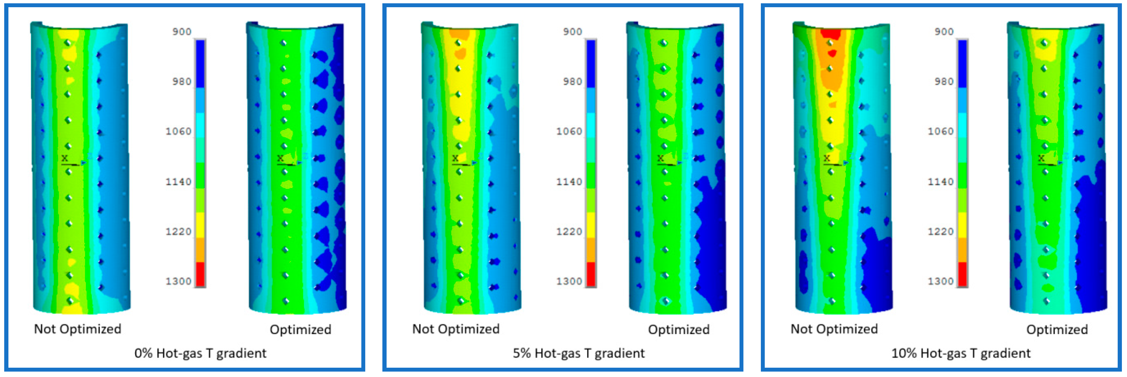
To open the discussion, results with 1st iteration optimized and not-optimized temperature profiles are plotted side-by-side. As shown in Figure 7, the optimized film holes after a single iteration reduce the variation in temperatures along the vane while decreasing the maximum temperature present. The optimization process is model-less and does not know that a skewed boundary condition is imposed in some configurations. The results indicate that the temperature distribution is smoother with optimized solution. The coolant use is also efficient as illustrated later in this section. For a +/− 5% temperature change for the external profile, the bottom-to-top increase in temperatures is apparent in nonoptimized solution. The optimized solution adjusted the hole sizes and thus the top-to-bottom temperature distribution is more uniform. With a +/−10% temperature variation, a greater fluctuation in temperatures is present in the nonoptimized solution. The optimized solution is better but note that at these extreme temperature variations, the hole size limitations got activated and therefore, the temperature distribution is better but not as smooth as other cases presented here. We are using hole size optimization and in another study, Kirollos and Povey [38,39] showed analytical solution of optimized uniform temperatures with adjusting the heat transfer coefficients of the cooling surfaces. Their guidance is helpful but is very difficult to implement. In most thermal designs, the heat transfer coefficient and the coolant temperature are difficult to manage or to implement; whereas, adjusting the physical dimension of holes or apertures are more doable. We have intentionally used fraction of mm in diameters, as the emerging additive manufacturing and other advances are making it feasible to make holes with different hole sizes in commercial production.

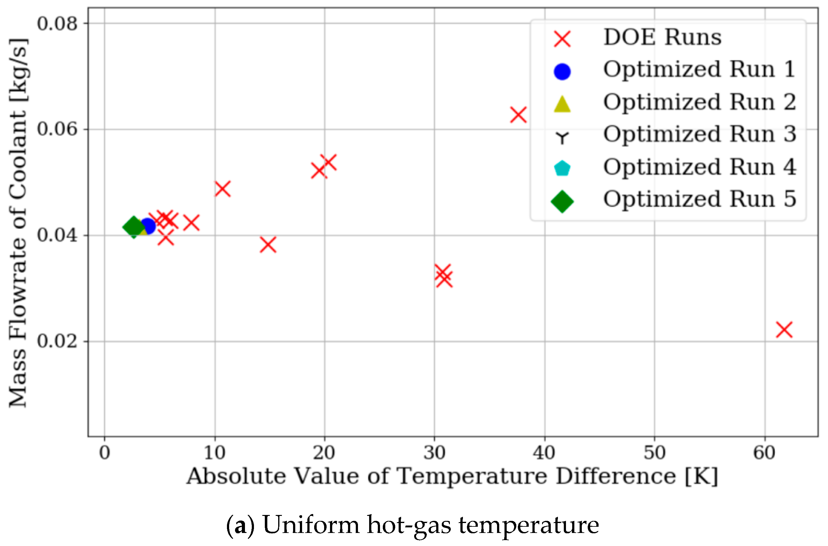
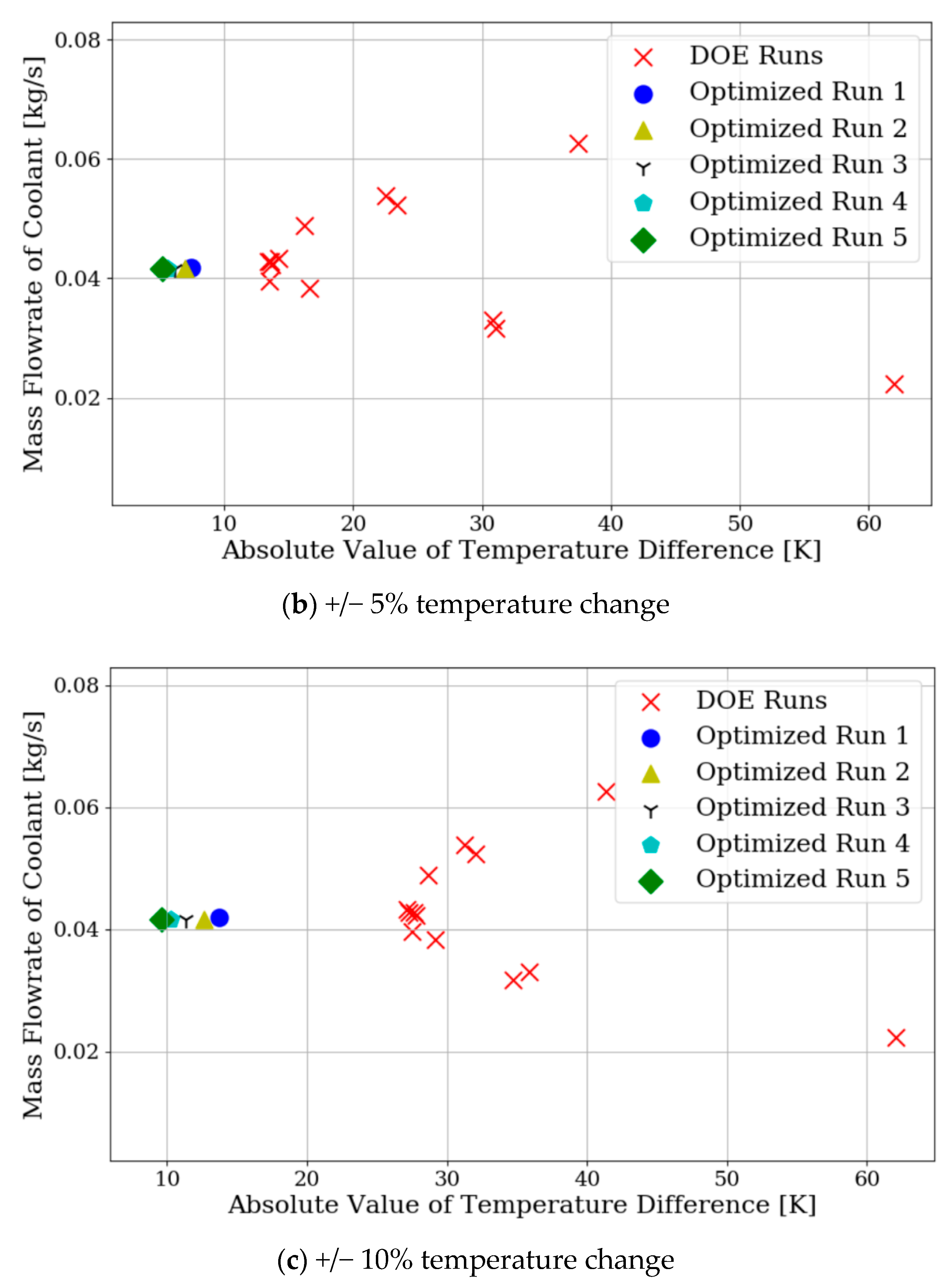
Less temperature variation with the least coolant usage is the objective and results are plotted in Figure 8. This figure plots absolute temperature difference on the x-axis, which is the average slice temperature minus the desired temperature. The range of temperature differences for DOE runs, which are the datasets used for training the model, are higher than the optimized solution; moreover, with skewed boundary temperature configurations, the difference in DOE sets is greater with greater skewness. This displays that the average difference is nearly zero for different optimized iterations and the outcome is robust as it does not deviate too much from zero, which is desired. For the given constraints on hole size and hole location, the coolant flow could not be lowered any further with more iterations, but the temperature differences and variations improved with each iteration. The training sample had an average temperature standard deviation of 32.6 K among the slices with 10% change, which is not shown in this plot, and the optimization process showed a marked improvement. For 10% hot-gas temperature boundary condition, the temperature variation improved as 16.8, 15.95, 14.84, 13.89, and 13.38 K with each iteration. Note that the proposed method replaces only one training sample in the existing 13 training samples based on performance and therefore, the improvement is slow. This perhaps can be improved with more research and new algorithm development.

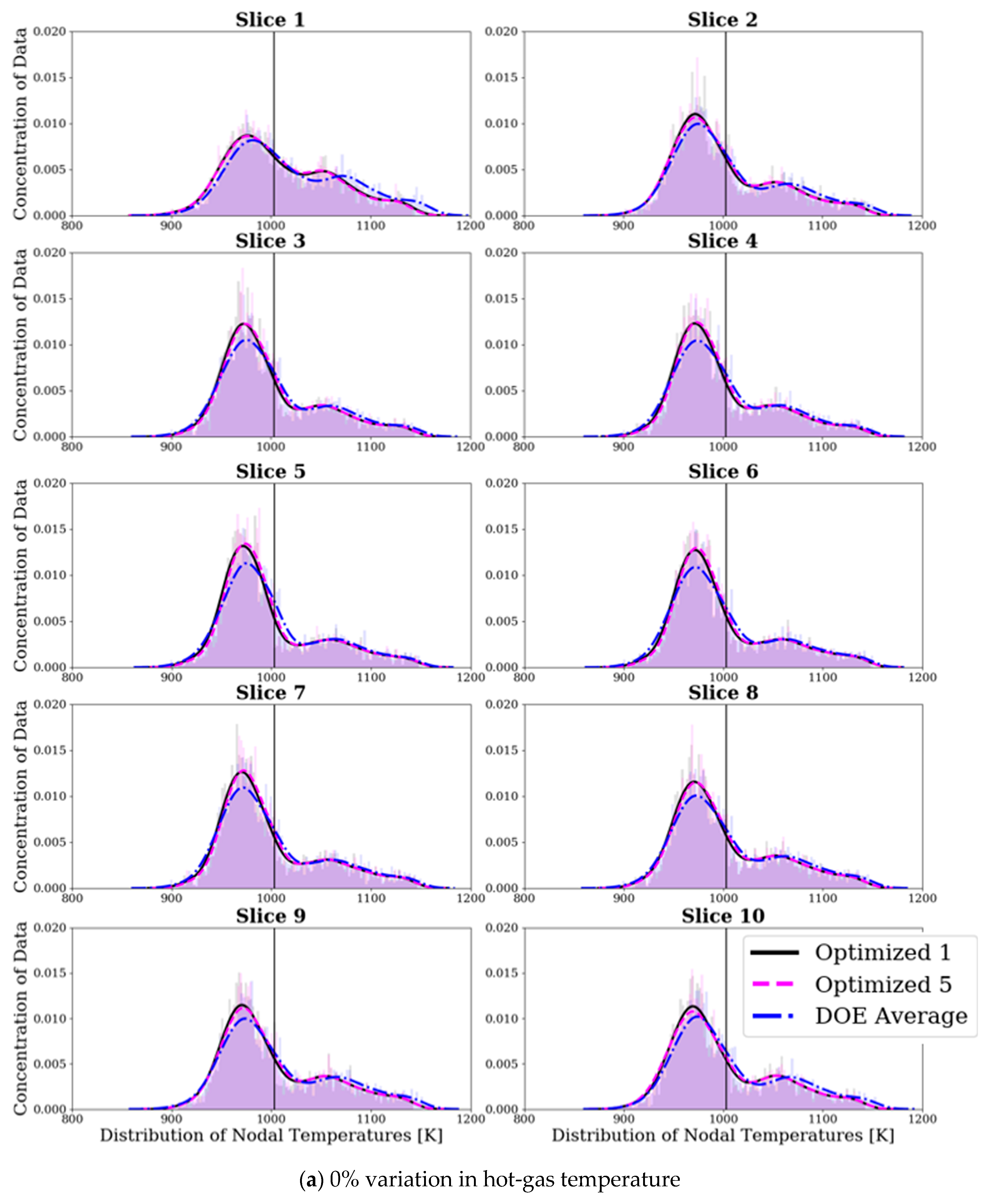
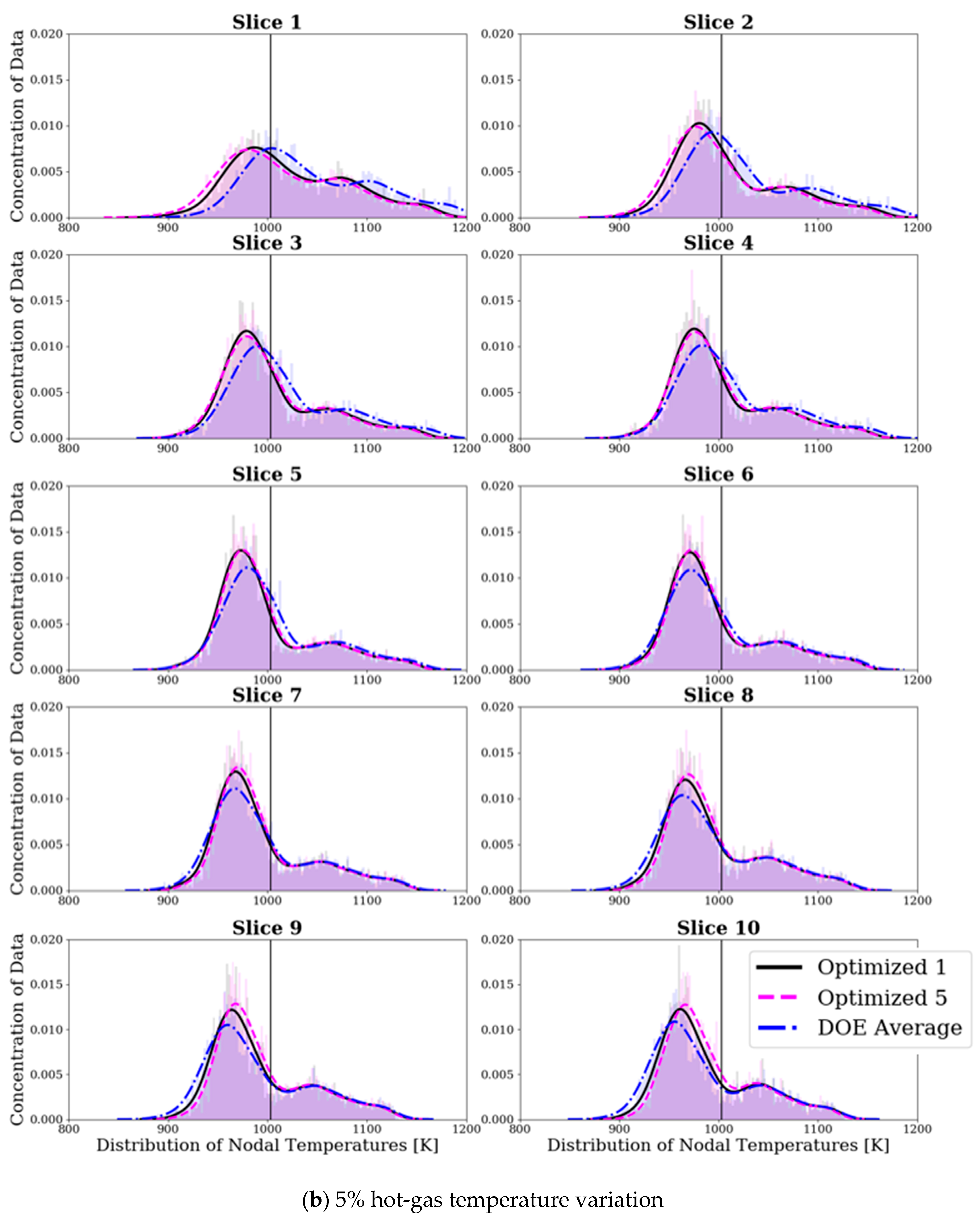
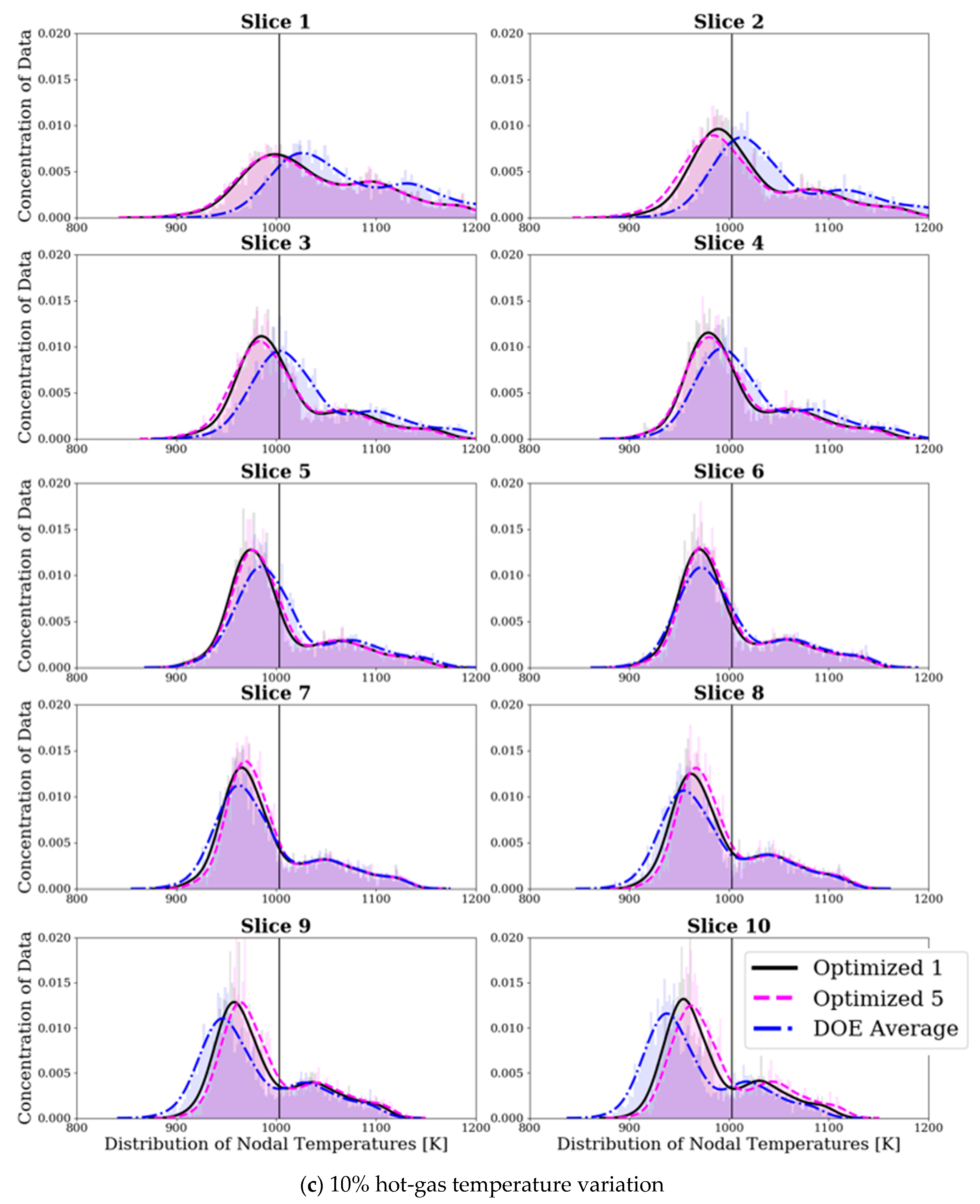
Figure 9 shows the reduction in standard deviation of metal temperatures in vane slices for optimized results. The reference starting distribution is marked as DOE (Design of experiments) sample. The average diameter of 3 mm is used to set that reference. Then distribution results from iteration 1 and iteration 5 are superimposed. These plots are probability distribution of nodal temperatures. All situations are simulated with the same mesh and therefore, effects from spatial variation or nodal densities are eliminated. Results indicate that the nodal distribution of optimized solutions reduces the standard deviation by increasing the peak and narrowing the distribution plots. Effect of boundary temperature gradient is very well illustrated in Figure 9b,c. The lower numbered slices have higher temperature at the hot-gas boundary; whereas, higher numbered slices have lower boundary temperatures and optimization process handled them differently without any additional adjustment from the designer. Results show that NORS process produces temperature distribution that is more suitable for the design goals. The vertical line in these plots is the desired average temperature. For this exercise, it was taken to be the average temperature of DOE. Results indicate that even one iteration produces a much better temperature distribution by shifting the peak closer to the limit and reducing the spread of the temperature distribution. It was also observed that this nodal temperature distribution has a double hump from the film cooling effectiveness and heat transfer coefficient distributions, known as bimodal distribution. A larger component with many more rows of film holes may get more humps in the distribution or the double hump may get a stronger secondary peak. NORS handled the double peak temperature distribution without difficulty.

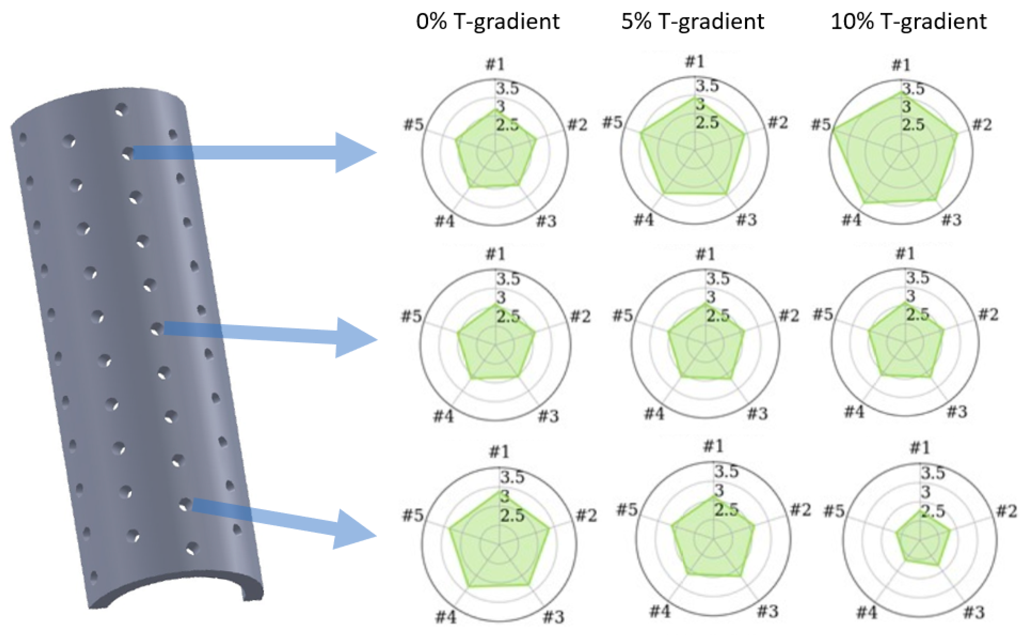
Figure 10 illustrates how NORS iterative procedure changes the local diameters. The first column of results shows the diameters with no variation of the boundary temperature, second column is with 5% variation and the third column is with 10% variation, as was illustrated in Figure 4. The rows of radar plots are for a given location as marked by arrows on the hole arrangement and iteration results are marked as #. As the boundary temperatures were hotter (top row) with skewed boundary conditions, optimized hole diameters got bigger; and as the boundary temperature dropped, the hole diameters automatically reduced as indicated by the bottom row. In NORS technique, one sample is replaced by the next best solution in each iteration. It is not a fast change, but by the 5th iteration, five lower performing hole sets were replaced from the training samples, and the hole diameters did not change drastically from iteration to iteration. Thus, it shows the robustness of the technique and shows that even with rough estimates in the initial DOE, the optimized values beginning from 1st iteration were close to the optimized values of the 5th iteration. There is more opportunity to get faster changes, but it could not be conclusively observed if the result obtained is the global best or a local best of many possible optimized solutions. However, for engineering purpose, the results obtained are encouraging and shows that an optimized distribution of hole diameters are feasible with a methodical approach rather than hunting it by trial and error.

7. Conclusions

An optimization process for nonlinear coupled systems is proposed with illustration of successful thermal simulation results based on a leading-edge of a turbine airfoil. The methodology includes a model-based analysis and a model-free optimization process. The model-based analysis is problem dependent and needs to have domain knowledge to build the input–output response system. The model-less routine does not need to know the science or technology involved in the model-based system. Model-free portion of the routine uses the input-output datasets to optimize on the desired output and it predicts what the input should be to get that output.

Three different boundary conditions are tested, and results are very promising. In all situations, the optimization outcome delivered significant improvement on desired temperature uniformity without sacrificing on the coolant usage. The metal temperature distributions show that the optimized FE nodal temperatures cluster around the desired temperature with less spread than the corresponding distribution observed with nonoptimized solutions. This NORS technique can be used in other engineering problems like statics and dynamics, or any system that can be modeled with unique output for given inputs. The optimization process is simple and does not require extensive computation resources. There are many ways to apply this NORS technique and improve on it, thus opening graduate and undergraduate learning and research opportunities. The design process as proposed is ready for industrial use without any modifications.