Pattern Recognition of DC Partial Discharge on XLPE Cable Based on ADAM-DBN

Abstract

Pattern recognition of DC partial discharge (PD) receives plenty of attention and recent researches mainly focus on the static characteristics of PD signals. In order to improve the recognition accuracy of DC cable and extract information from PD waveforms, a modified deep belief network (DBN) supervised fine-tuned by the adaptive moment estimation (ADAM) algorithm is proposed to recognize the four typical insulation defects of DC cable according to the PD pulse waveforms. Moreover, the effect of the training sample set size on recognition accuracy is analyzed. Compared with naive Bayes (NB), K-nearest neighbor (KNN), support vector machine (SVM), and back propagation neural networks (BPNN), the ADAM-DBN method has higher accuracy on four different defect types due to the excellent ability in terms of the feature extraction of PD pulse waveforms. Moreover, the increase of training sample set size would lead to the increase of recognition accuracy within a certain range.

1. Introduction

HVDC (High Voltage Direct Current) transmission has the advantages of low line cost, not being restricted by synchronous stability problems, thus the project of DC cable has developed rapidly in recent years [1,2,3]. With the excellent performance of DC cross-linked polyethylene (XLPE) cables, the usage of XLPE cables has gradually outstripped the oil-filled and impregnation paper cables since its first adoption in Sweden [4]. In order to improve the stability and reliability of DC transmission, technology such as online detection and condition evaluation of cables as well as accessories has become a great concern for scholars.

The accumulation of space charge inside the polymer leads to local electric field distortion, which may result in partial discharge (PD), especially in insulation defects. Thus, the PD detection is often used for XLPE cable detection to evaluate the operating condition of the cable. There are lots of literatures about PD researches of AC XLPE cable, but few standards or recognized diagnose methods for DC cable [5,6]. PD analysis methods can be divided into phase resolved partial discharge (PRPD) mode and time resolved partial discharge (TRPD) mode [7]. Because the PD signal under DC has no phase information, the time interval between two adjacent discharge Δt is usually used as an important characteristic parameter [8]. Yang achieved pattern recognition from a H(q, Δt) feature map by using the sparse representation classification technology based on the compressed sensing theory [9]. Mazroua used a neural network for training and identification according to characteristics such as average current of discharge, repetition rate, and discharge energy [10]. Ma proposed the time-frequency analysis of the waveform to pattern recognition by using fuzzy C mean clustering and minimum two-way support vector machine [11]. Morette successfully implemented supervised and unsupervised classification methods based on feature extraction from PD [12,13]. However, based on features extracted from TRPD, the usage of neural networks, support vector machines, and other algorithms takes a lot of time to study how to extract features efficiently. The deep belief network (DBN) is a deep learning model with excellent feature learning ability, outstanding performance in data degradation and feature recognition, which is widely used in image processing, speech recognition [14,15,16]. Wang applies the DBN to the hybrid fault diagnosis method in transformer oil [17], and Zhang uses DBN to identify the analog circuit incipient faults [18]. Both of them have good performance and prove that the deep learning method has strong characteristic learning ability based on the original data. However, the effect of the PD diagnosis for DC XLPE cable based on DBN has not been tested because of the limited data capacity.

In this paper, a modified DBN algorithm based on DC PD pulse waveforms is proposed to achieve the pattern recognition of DC cable insulation defects. First, the PD signals of typical insulation defect cables are collected through the DC experimental platform. Second, the PD pulse waveform is pre-processed using the Canny algorithm and used as an input sample for the classification model. Third, a DBN recognition model optimized by the adaptive moment estimation (ADAM) algorithm is built to achieve the pattern recognition of different defect types. Finally, compared with the artificial feature recognition methods, the effect of classification methods on various defects and the effect of training sample capacity on the classification models are analyzed. The experimental results show that the proposed method improves the accuracy of the recognition of DC XLPE cable insulation defects.

2. Deep Belief Networks

The deep belief network is a non-convolution generation model proposed by Hinton et al. in 2006 which solves the problem that the depth model was difficult to optimize. The deep belief network consists of a multi-layered restricted Boltzmann machine (RBM). It uses the contrastive divergence (CD) algorithm for unsupervised training of RBM and then uses supervised training for tuning of the entire DBN network.

2.1. RBM

The RBM is an undirected probability graph model consisted of the visual layer and the implied layer group, where there is no connection between the cells in the visual layer or the implied layer. The RBM is an energy-based model consisting of a visual layer v and a hidden layer h, with RBM’s energy function [17]:

$$E_{\theta }(v,h)=-{\displaystyle \sum _{i=1}^{n_v}{a}_i{v}_i}-{\displaystyle \sum _{j=1}^{n_h}{b}_j{h}_j-{\displaystyle \sum _{i=1}^{n_v}{\displaystyle \sum _{j=1}^{n_h}{v}_i{w}_{ij}{h}_j}}}$$

(1)

where θ = {w = (w_ij)_n×m, a = (a_i)_n, b = (b_j)_m} is the parameter of the RBM model, a_i and b_j are the biases of the visible unit v_i and the hidden unit h_j, respectively, w_ij is the connection weight between the visible unit v_i and the hidden unit h_j, and n_v and n_h are the number of visible unit v_i and hidden unit h_j, respectively.

The joint probability distribution is specified by the energy function [19]:

$$P_{\theta }(v,h)=\frac{1}{Z}\exp (-E(v,h))$$

(2)

where Z is a normalized factor called an allocation function:

$$Z_{\theta }={\displaystyle \sum _v{\displaystyle \sum _h\exp (-E(v,h))}}$$

(3)

The state of the hidden elements in RBM is independent of each other, and when given the visible unit v, the probability that the hidden unit h is activated (set to 1) is [20]:

$$P_{\theta }(h_j=1|v)=\mathrm{sigmoid}(b_j+{\displaystyle \sum _{i=1}^{n_v}{w}_{ij}{v}_i)}$$

(4)

Similarly, when the state of hidden unit h is determined, the probability that the visible unit v is activated is [18]:

$$P_{\theta }(v_i=1|h)=\mathrm{sigmoid}(a_i+{\displaystyle \sum _{j=1}^{n_h}{w}_{ji}{h}_j)}$$

(5)

where sigmoid = (1 + exp(−x))⁻¹ is an activation function that maps x to the interval of (0,1).

For the RBM model given the number of explicit elements and hidden elements, it is necessary to determine the parameter θ through training, where the training goal is to make the data reconstructed from the RBM model under the control of the parameter θ as consistent as possible with the given training sample data. Because the fractionation function of RBM, Z_θ, is difficult to calculate by simple method, this paper uses the comparative dispersion (CD) algorithm proposed by Hinton in 2002 to carry out rapid unsupervised training of RBM to solve the optimal value of the θ [21].

The CD algorithm first initializes the parameters θ randomly, uses the training sample as a visible unit v⁰, and calculates the hidden unit h⁰ according to Equation (4). Then, it reconstructs the visible unit v¹ according to the Equation (5) and recalculates the hidden unit h¹. Each parameter update formula is shown in Equation (6):

$$\{\begin{array}{l}\Delta w_{ij}=\epsilon (<v_i^0{h}_j^0>-<v_i^1{h}_j^1>)\\ \Delta a_i=\epsilon (<v_i>-<v_i^1>)\\ \Delta b_j=\epsilon (<h_j>-<h_j^1>)\end{array}$$

(6)

where $\epsilon$ is the learning rate of comparing dispersion method, and $<\cdot >$ is mathematical expectation.

In the actual training, due to the large sample size, the random sampling of training samples for RBM was trained in several small quantity batches to improve the computational efficiency. Suppose the number of the random sample size is N, the update formula for the k-th training is:

$$\{\begin{array}{l}{w}_{ij,k}=w_{ij,k-1}+\epsilon [{\displaystyle \sum _{n=1}^N(v_{i,n}{h}_{j,n}-v_{i,n}^{\prime }{h}_{j,n}^{\prime })/N}]\\ a_{i,k}=a_{i,k-1}+\epsilon [{\displaystyle \sum _{n=1}^N(v_{i,n}-v_{i,n}^{\prime })/N}]\\ b_{j,k}=b_{j,k-1}+\epsilon [{\displaystyle \sum _{n=1}^N(h_{j,n}-h_{j,n}^{\prime })/N}]\end{array}$$

(7)

2.2. Pre-Training of DBN

The classification model based on the DBN is stacked with several RBMs and consists of an input layer, several hidden layers and an output layer consisting of the Softmax classifier. The structure is shown in Figure 1.

Each of the two adjacent layers in the input layer and the hidden layer constitutes an RBM, as shown in Figure 1. The RBM₁ consists of the visible unit v¹ and the hidden unit h¹, which is also acting as the visible unit v² of RBM₂, and so on, the visible unit v^k of RBM_k is the hidden unit h^k−1 of RBM_k−1. The top layer of the network is the Softmax classifier, which maps the DBN from the features extracted from the original data to the category to be divided.

In DBN, RBM network is unsupervised trained layer by layer. First, using the CD algorithm training the input data v⁰ is trained to obtain RBM₁ parameters θ₁. Then, using the activation probability of h¹ as training data, RBM₂ is trained to get the θ₂, and so on. Finally, get the pre-trained network weight and the bias.

2.3. Supervised Fine-Tuning Based on ADAM

RBM training is carried out independently, so the model parameters are optimal in RBM locally. Therefore, the parameters need to be fine-tuned at the end of the pre-training phase. For a given set of training samples {x, y}, the relationship between input and output can be expressed as:

$${\widehat{y}}_i=f(x_i,\theta )$$

(8)

where f is a nonlinear function; x_i is the i-th sample in the training sample $x=[x_1,x_2,\cdots ,x_n]$; ${\widehat{y}}_i$ is the label of i-th sample mapped in the DBN model.

Use the average of the cross entropy of the predicted and actual values as the function of error loss:

$$J(\theta )=-\frac{1}{N}{\displaystyle \sum _{i=1}^N{y}_i\log ({\widehat{y}}_i)}$$

(9)

where N is the number of the training samples and y_i is the actual value of i-th sample.

The supervised fine-tuning of DBN usually uses the gradient drop method and conjugate gradient descent method. But it is difficult to select the appropriate learning rate and seems to converge to local optimal. The adaptive moment estimation (ADAM) algorithm was proposed by Kingma in 2015 and has excellent performance in dealing with sparse gradients and unsteady states, requiring only a small amount of tuning [22]. When get the network parameters θ_k of the k-th iteration, calculate the gradient g_k = ∇J(θ_k), update the partial first-order moment estimation m_k+1 and the partial second-order moment estimation v_k+1:

$$\{\begin{array}{l}{m}_{k+1}={\beta }_1{m}_k+(1-{\beta }_1)g_k\\ v_{k+1}={\beta }_2{v}_k+(1-{\beta }_2)g_k^2\end{array}$$

(10)

Then, calculate the first-order moment deviation ${\widehat{m}}_{k+1}$ and the second-order moment deviation ${\widehat{v}}_{k+1}$:

$$\{\begin{array}{l}{\widehat{m}}_{k+1}=m_{k+1}/(1-{\beta }_1^{k+1})\\ {\widehat{v}}_{k+1}=v_{k+1}/(1-{\beta }_2^{k+1})\end{array}$$

(11)

The network parameters are updated:

$${\theta }_{k+1}={\theta }_k-\alpha {\widehat{m}}_{k+1}/(\sqrt{{\widehat{v}}_{k+1}}+\tau )$$

(12)

where α is the step length, τ is the stable constant.

ADAM algorithm parameters are set according to the reference [20], which α = 0.001, τ = 10⁻⁸, β₁ = 0.9, β₂ = 0.999. ADAM makes full use of the adaptive learning rate of first-order moment mean and second-order moment mean to alleviate the problem of local suboptimal convergence and saddle point residence.

3. Cable PD Pattern Recognition Based on ADAM-DBN

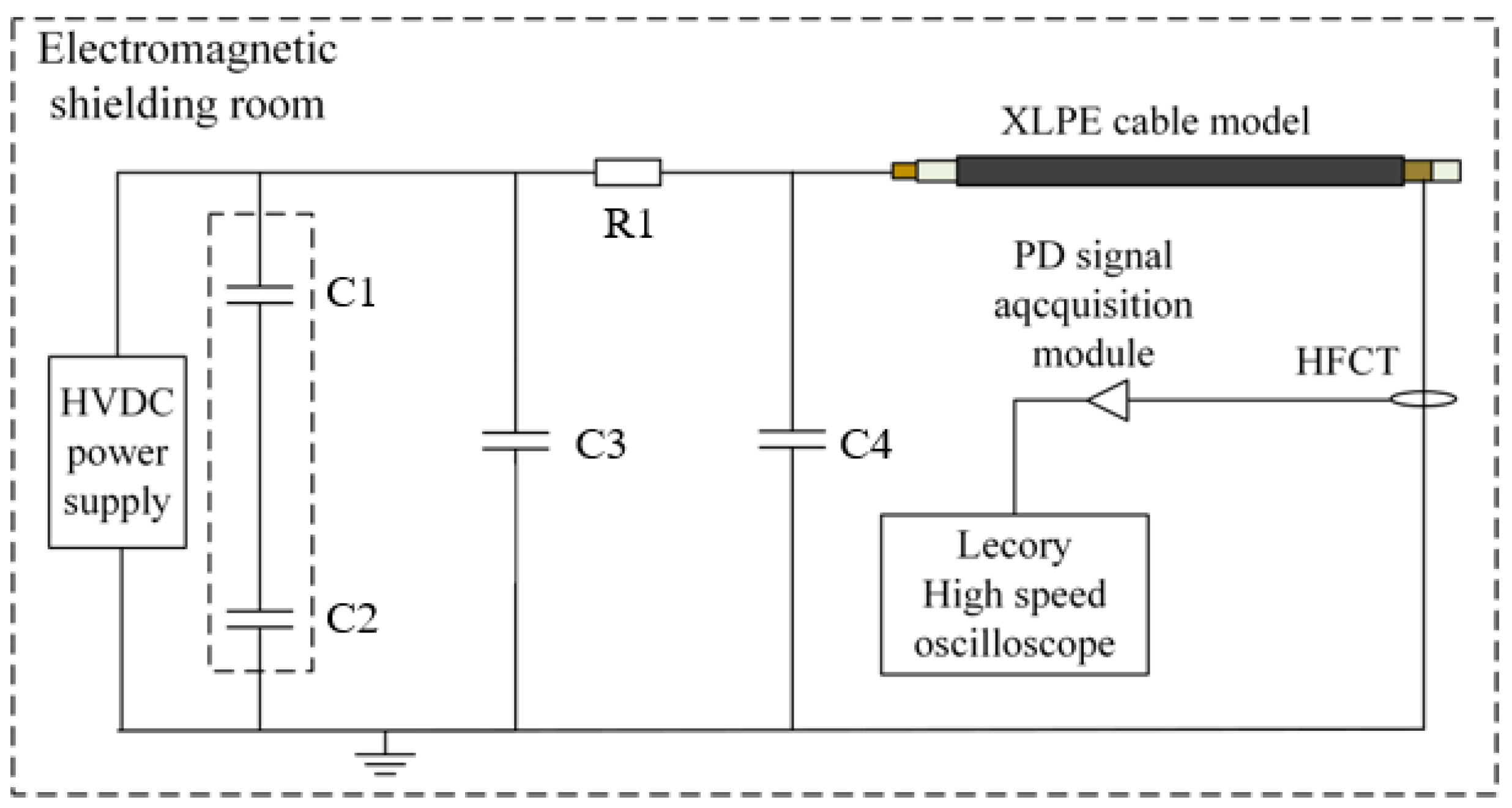
3.1. Insulation Defect Design and Test System Construction

Based on the common insulation faults in the actual operation of XLPE cables, this paper designs four typical defect models: (1) Conductor burrs as defect C1. A 1.5 mm long metal needle is attached to the outer surface of the XLPE insulation, with one end touching the cable copper core and the other hanging inside the XLPE insulation. (2) External semi-conductive layer residue as defect C2. In the process of peeling the semi-conductive layer, remain the 3 mm wide and 30 mm long semi-conductive layer on the main insulated surface. (3) Internal air gap as defect C3. Manufacture several micro-holes over the XLPE cable insulation interface to allow a small amount of air to enter the inside of the insulation. Then the seal is applied to the hole and surrounding with epoxy resin. (4) Scratch on the insulation surface as defect C4. Scratches are made along the axial axis on the surface of the XLPE cable insulation, with a width of 1 mm and a depth of 1 mm. The typical insulation defects for XLPE cables are shown as Figure 2.

The experimental system is shown in Figure 3. The experiment was carried out in the shielding chamber and the environment remained in the range of (293 ± 5) K. The high-voltage DC source used in the experiment is a 5 kVA/200 skV DC generator, C1 and C2 are 200 kV/100 pF DC divider, C3 is 200 kV/10,000 pF filter capacitor, R1 is 10 kΩ protective water resistance, C4 is 150 kV/300 pF coupling capacitor. This experiment used the HFCT detection system to detect partial discharges. The passband of the Rogowski coil is 3 MHz to 50 MHz. The Lecroy high-speed oscilloscope has a bandwidth of 2 GHz and a maximum sampling rate of 20 GS/s. The HFCT detection coil is clamped on the ground wire of the copper shielding layer of the cable, and then connected to the oscilloscope through the PD signal acquisition module. The rise time of PD pulse current is usually nanosecond order, the pulse duration is about 1000 ns. The sampling rate of the oscilloscope is set to 200 MSa/s, which meets the requirements of the Nyquist sampling theorem. Each cable defect model is tested under constant DC voltage, maintain the applied voltage of the cable at partial discharge inception voltage. In the pressure test, a constant voltage test was carried out at five voltage levels. The voltage level gradient was about 4.5 kV, and each voltage gradient was maintained for at least 20 min.

3.2. Sample Collection

The four defect models were connected into the system individually, and then slow boost the voltage when PD was relatively stable. The PD pulse waveform signal data was collected through HFCT. The measured pulse waveform signal is shown in Figure 4, the oscilloscope acquisition PD signal contains redundant information before and after the pulse time. Therefore, this paper introduces the modified Canny edge detection operator to pre-process the pulse waveform and intercepts the part of the red area in the figure so as to maximize the information efficiency.

Canny edge detection has the advantages of strong anti-noise interference, easy detection of weak edges [23]. The steps of using Canny algorithm to extract effective information of waveform are as follows. (1) Use Gaussian filtering to smooth the waveform. (2) Take the waveform derivative, perform non-maximum value suppression, and retain only the derivative maximum value point. (3) For dual-threshold detection, suppress the derivatives if below the low threshold suppression, mark as strong edge points if above the high threshold, and mark as weak edge points otherwise. (4) Suppress the isolated weak edge point and the weak edge point if there is no strong edge point nearby.

After determining the starting point of the discharge waveform, the discharge waveform is intercepted according to the length of the waveform and the sample rate, which is set to 600 in this article. Due to the different stable discharge voltages of different defects, the amplitude is normalized after intercepting the waveform.

The pre-processed PD waveform of four typical defects is shown in Figure 5. As shown in figure, the discharge current of C1 and C2 have 3 or 4 fluctuation approximately, and the amplitude decays faster, where the decline of current amplitude fluctuation of C2 decrease rapidly. The current waveforms of C3 and C4 are similar, have about 6–7 triangularly fluctuations, and the current amplitude decay is slow, where the current of C4 becomes an irregular violent jitter at a later stage.

The pre-processed current waveform is used as sample data, and the sample dimension is the signal length intercepted. A total of 6400 samples were collected, where 1600 samples of discharge signals for each type of insulation defect. In addition, 14 characteristics of the PD current waveforms are extracted, such as skewness degree S_k, steepness K_u, number of local peak P_k, rise time of waveform T_r, peak time T_p, drop time T_d, pulse width T_w, pulse mean u_t, pulse variance σ_t², frequency of frequency domain characteristic spectral peak p, amplitude of spectral peak F, number of spectral peak M_p, spectral mean u_f, spectral variance σ_f², as manual extraction features to be compared with the method proposed in this paper.

3.3. Pattern Recognition Step Based on ADAM-DBN

The PD pattern recognition step of DC cable based on the ADAM-DBN are shown as follows:

(1)

The original data are pre-processed and divided proportionally into training sets and sample sets.

(2)

Construct the DBN recognition model, pre-train it with CD algorithm, and get the pre-trained network parameters of the identification model.

(3)

Using the ADAM algorithm, the DBN model is supervised trained by training sample label, fine-tuning the network parameters to make the model optimized.

(4)

Use the test data set as input to inspect the trained DBN model.

4. Experimental Analysis

4.1. Experimental Evaluation Indicators

Accuracy and recall are used as indicators to measure the effectiveness of various methods of diagnosing insulation defects. In multi-category problems, accuracy represents the proportion of all samples correctly predicted to the total sample:

$$a=\frac{card({\displaystyle \sum X_i)}}{card({\displaystyle \sum C_i)}}$$

(13)

Recall rate represents the proportion of the actual type of sample that was correctly determined for that type:

$$r=\frac{card(X_i)}{card(C_i)}$$

(14)

where, X_i represents a collection of the actual type and recognized type are all i and C_i is the collection of the actual type of i.

Through the analysis of accuracy and recall rate, we can not only evaluate the overall effectiveness of the pattern recognition method, but also examine the specific identification effect of the pattern recognition method for each defect, and analyze the application of the algorithm to different defects.

4.2. Structure and Parameter Settings

The initial bias of parameters in the DBN model are set to 0, and the initial weight uses the random number generated by the Gaussian distribution, where the expectation of Gaussian distribution is set to 0, the standard deviation is set to the inverse of the mean square root value of the number of cells in the visual layer, the batch size of the pre-training stage is 100, the RBM learning rate is 0.1, and the learning cycle of the fine-tuning stage is preset 200. Because the hidden layer structure and learning cycle have a great influence on the recognition accuracy, this paper determines the specific value through experiments.

The number of hidden layers of the model and the number of hidden units per hidden layer are obtained by the enumeration method. Thereby, first, a hidden layer is set for the model, the number of hidden units is gradually increased, the average accuracy of 10 experiments is recorded as a performance indicator, then the optimal value of the number of hidden units is determined. Moreover, add one more hidden layer and choose the optimal number of hidden units of second hidden layer, until the validation score is no longer improved.

The relationship between the number of hidden units and the validation score is shown in Figure 6, where N indicates that there is one hidden layer and the number of hidden units is set to N, and 50-N indicates that there is two hidden layers and the number of hidden units of each layer are 50 and N respectively. Considering the computational efficiency, the network structure of this paper contains two hidden layers, where the numbers of hidden units in the first and second layers are both set to 50.

After determining the structure of the hidden layer, the effect of the learning cycle on the recognition effect is analyzed. Figure 7 shows the validation score of the learning cycle set to 20–400 (interval 20). This shows that the validation score increases significantly with the increase of the learning cycle when the learning cycle is less than 200, but increases insignificantly after 200. Identifying efficiency and computing costs, it is reasonable to set a learning cycle of 200.

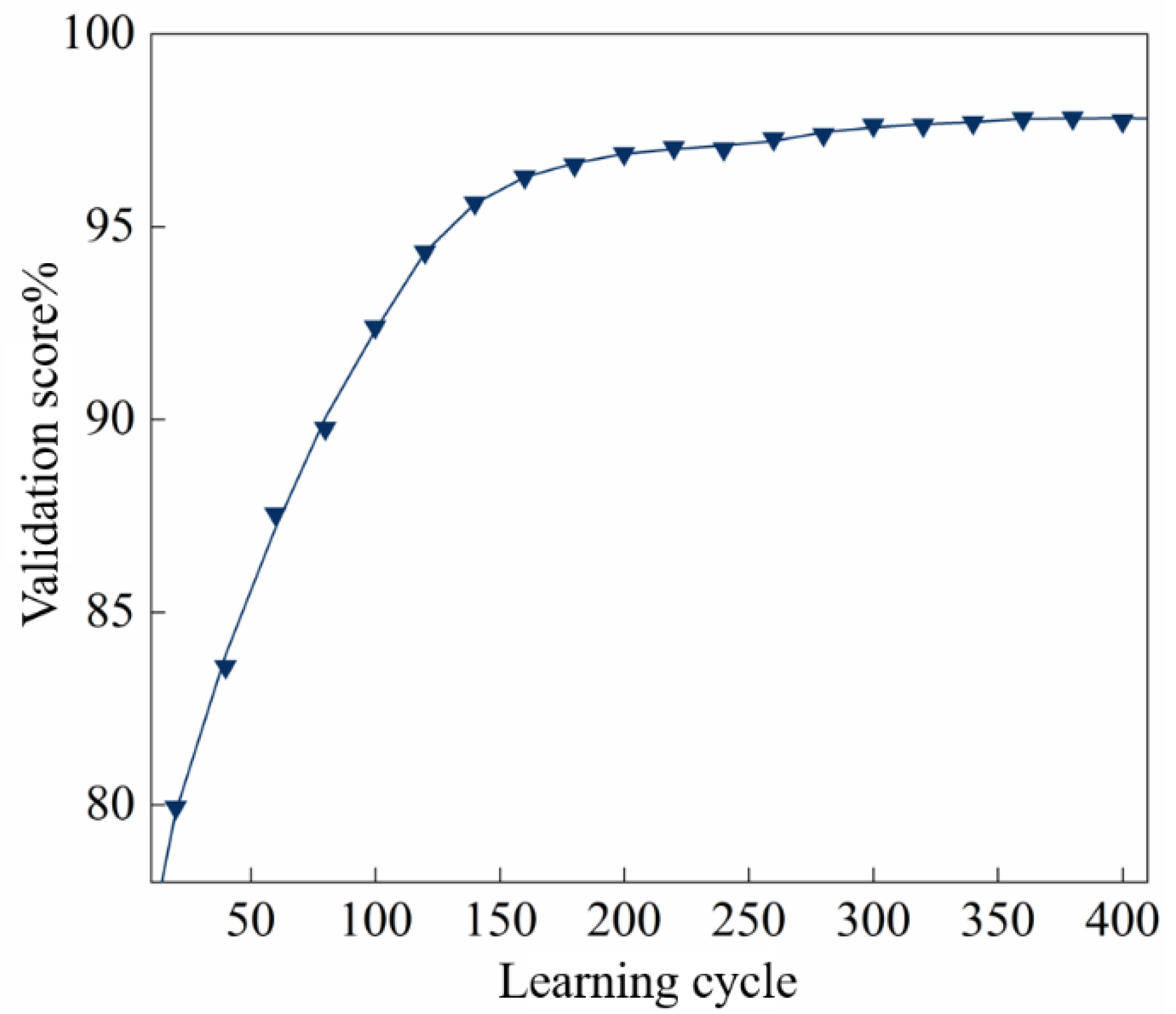
4.3. Results Analysis

We compare ADAM-DBN with naïve Bayes (NB), K-nearest neighbor (KNN), support vector machine (SVM) and back propagation neural networks (BPNN) to evaluate the effectiveness of pattern recognition. Here, the Lidstone smoothing parameters of the NB model are α = 2ⁿ, n = −10, −9, …, 10. KNN model uses European distance as the criterion for judging and the neighbors are set to 20. The SVM model uses radial basis function (RBF), which takes σ² = 2ⁿ, where in n = −10, −9, ... 0, …, 10, as the error penalty parameter, and for the parameter of the optimal test accuracy, choose σ² = 4 as the setting parameter. BPNN model has 14 nodes of input layer, 10 nodes of hidden layer, learning rate 0.01, learning cycle 200. As a comparison of the traditional DBN model, RBM learning rate 0.1, fine-tuning stage learning rate 0.4, fine-tuning stage learning cycle 200, using method of Section 3.2 to obtain the hidden layer structure, which has two hidden layers and 50 hidden units each layer.

The pre-processed data sample set is divided into training sets and testing sets by 2:8, as the input of the ADAM-DBM model and the traditional DBN model. The 14 feature sample sets are also divided into training sets and testing sets by 2:8, as the input of the NB, KNN, SVM, and BPNN models. Figure 8 shows the confusion matrix of different methods, where each row represents the actual type, each column represents the predicted type, and the values in the figure represent the proportion of the sample type identified as the sample type in the column. All correct identification results are on the diagonal, and the error is distributing outside the diagonal. In addition to giving the specific recall rate of each defect, the specific error rates of the defect type being misidentified are also given.

As can be seen from Figure 8, the overall identification accuracy of ADAM-DBN model is the highest, where the identification accuracy of the four types of defects has reached more than 95%. Moreover, the accuracy rate of identifying C1 and C2 is more than 98.5%. Compared with the traditional DBN method, ADAM has a higher efficiency of monitoring and optimization of DBN network weight, and the network’s mapping of the original signal effectively removes redundant information, so the accuracy of recognition is further improved.

NB, KNN, SVM, BPNN, and DBN method have good overall prediction effectiveness, especially for the identification of defect C2, but performance poor at the identification of C3 and C4. The identify accuracy of C3 and C4 of NB, KNN is less than 90%, and accuracy of SVM, BPNN is less than 92%. This is because C3 and C4 both are situation that part of the insulation is filled with air, so there is a certain similarity between C3 and C4. From Figure 8, we can also see that C3 and C4 are the main types of misidentification of each other, indicating that the characteristics of artificial extraction perform good in C2, but lacks in the identification ability in C3 and C4.

In order to analyze the effect of training data scale on the recognition accuracy, 4000 of the 6400 samples were used as test data set, and the remaining samples were treated as training sets of 400, 800, 1200, 1600, 2000, and 2400, respectively. The results of identification accuracy of NB, KNN, SVM, BPNN, DBN, and ADAM-DBN under six different scales of training data set are shown in

Table 1. Recognition accuracy on different scales of training sample sets.

Training Set	Recognition Accuracy%
	NB	KNN	SVM	BPNN	DBN	ADAM-DBN
400	90.4	93.8	94.6	93.9	92.8	93.8
800	90.1	94.3	95.3	94.5	95.1	95.9
1200	90.4	94.7	95.9	95.2	96.1	96.8
1600	90.5	94.8	96.0	95.3	97.0	98.0
2000	90.6	95.0	96.1	95.4	97.2	98.2
2400	90.5	95.1	96.1	95.6	97.3	98.4

.

From Table 1, it can be seen that with the increase scale of training set, recognition accuracy of KNN, SVM, BPNN, traditional DBN and ADAM-DBN is increasing, but accuracy of NB has not significantly improved. In the case of small training set, the recognition accuracy of DBN is similar to that of other classification algorithms. However, with the increase of the number of training set, the characteristics of the local pulse waveform extracted by the deep learning network are more comprehensive, thus the recognition accuracy of DBN is obviously better than other four methods. At the same time, the modified DBN model supervised fine-tuned by the ADAM algorithm converges faster and the recognition accuracy is higher than other methods on the same training scale.

5. Conclusions

In this paper, a PD pattern recognition method of DC XLPE cable based on DBN algorithm is proposed to distinguish the different types of defect. Using the PD signal data collected by different artificial defects as input, the pattern recognition effect is analyzed, and the results are shown below:

• The Canny operator is used to pre-process the PD pulse waveform of the XLPE cable. The modified DBN model supervised fine-tuned by the ADAM algorithm is trained to get the pattern recognition result.
• Compared with the NB, KNN, SVM, and BPNN algorithms, ADAM-DBN can unsupervised extract the characteristic information contained in the PD pulse waveforms. And the recognition accuracy of the typical insulation defects in DC XLPE cables is higher than other methods.
• In the experiment, it is found that the traditional classification method based on statistical characteristics performs not so well in the identification of air gap and scratch defects. However, the pattern recognition method based on DBN can effectively characterize the intrinsic relationship between the insulation defect and the PD pulse current waveforms, and have a better recognition effect on all kinds of defects.
• With the increase of training sample size, the recognition accuracy of DC cable based on ADAM-DBN is increased, and the recognition effect is better than that of traditional DBN and other classification methods.

References

1. Du, B.X.; Li, Z.L.; Yang, Z.R.; Li, J. Application and Research Progress of HVDC XLPE Cables. High Volt. Eng. 2017, 43, 344–354. [Google Scholar]
2. Thue, W.A. Electrical Power Cable Engineering, 3rd ed.; Taylor and Francis: Abingdon, UK, 2012. [Google Scholar]
3. Gregory, B. Cable technology and applications in the 21st century. IEEE Power Eng. Rev. 2000, 20, 6–7. [Google Scholar] [CrossRef]
4. Kaminaga, K.; Ichihara, M.; Jinno, M.; Fujii, O.; Fukunaga, S.; Kobayashi, M.; Watanabe, K. Development of 500-kV XLPE cables and accessories for long-distance underground transmission lines. V. Long-term performance for 500-kV XLPE cables and joints. IEEE Trans. Power Deliv. 1996, 11, 1185–1194. [Google Scholar] [CrossRef]
5. Xu, Y.; Gu, X.; Liu, B.; Hui, B.; Ren, Z.; Meng, S. Special requirements of high frequency current transformers in the on-line detection of partial discharges in power cables. IEEE Electr. Insul. Mag. 2016, 32, 8–19. [Google Scholar] [CrossRef]
6. He, W.; Wang, Q.; Huang, C.; Li, H.; Liang, D. A Cost-Effective Technique for PD Testing of MV Cables Under Combined AC and Damped AC Voltage. IEEE Trans. Power Deliv. 2018, 33, 2039–2040. [Google Scholar]
7. Oyegoke, B.; Birtwhistle, D.; Lyall, J. Condition assessment of XLPE cable insulation using short-time polarisation and depolarisation current measurements. IET Sci. Meas. Technol. 2008, 2, 25–31. [Google Scholar] [CrossRef]
8. Fromm, U. Interpretation of partial discharges at dc voltages. IEEE Trans. Dielectr. Electr. Insul. 1995, 2, 761–770. [Google Scholar] [CrossRef]
9. Yang, F.; Sheng, G.; Xu, Y.; Hou, H.; Qian, Y.; Jiang, X. Partial discharge pattern recognition of XLPE cables at DC voltage based on the compressed sensing theory. IEEE Trans. Dielectr. Electr. Insul. 2017, 24, 2977–2985. [Google Scholar] [CrossRef]
10. Mazroua, A.A.; Salama, M.M.A.; Bartnikas, R. PD pattern recognition with neural networks using the multilayer perceptron technique. IEEE Trans. Electr. Insul. 1993, 28, 1082–1089. [Google Scholar] [CrossRef]
11. Ma, H.; Saha, T.K.; Ekanayake, C. Statistical learning techniques and their applications for condition assessment of power transformer. IEEE Trans. Dielectr. Electr. Insul. 2012, 19, 481–489. [Google Scholar] [CrossRef] [Green Version]
12. Morette, N.; Ditchi, T. Oussar, Feature Extraction and Ageing State Recognition using Partial Discharges in Cables under HVDC. Electr. Power Syst. Res. 2020, 178, 106053. [Google Scholar] [CrossRef]
13. Morette, N.; Heredia, L.C.; Ditchi, T.; Mor, A.R.; Oussar, Y. Partial discharges and noise classification under HVDC using unsupervised T and semi-supervised learning. Int. J. Electr. Power Energy Syst. 2020, 121, 106129. [Google Scholar] [CrossRef]
14. Liu, F.; Jiao, L.; Hou, B.; Yang, S. POL-SAR Image Classification Based on Wishart DBN and Local Spatial Information. IEEE Trans. Geosci. Remote Sens. 2016, 54, 3292–3308. [Google Scholar] [CrossRef]
15. Zhang, X.; Pan, X.; Wang, S. Fuzzy DBN with rule-based knowledge representation and high interpretability. In Proceedings of the 2017 12th International Conference on Intelligent Systems and Knowledge Engineering (ISKE), Nanjing, China, 24–26 November 2017; pp. 1–7. [Google Scholar]
16. Bengio, Y. Learning deep architectures for AI. Found. Trends Mach. Learn. 2009, 2, 1–127. [Google Scholar] [CrossRef]
17. Wang, T.; He, Y.; Shi, T.; Li, B. Transformer Incipient Hybrid Fault Diagnosis Based on Solar-Powered RFID Sensor and Optimized DBN Approach. IEEE Access 2019, 7, 74103–74110. [Google Scholar] [CrossRef]
18. Zhang, C.; He, Y.; Yuan, L.; Xiang, S. Analog Circuit Incipient Fault Diagnosis Method Using DBN Based Features Extraction. IEEE Access 2018, 6, 23053–23064. [Google Scholar] [CrossRef]
19. Hinton, G.E. A practical guide to training restricted Boltzmann machines. Momentum 2012, 9, 599–619. [Google Scholar]
20. Hinton, G.; Deng, L.; Yu, D.; Dahl, G. Deep neural networks for acoustic modeling in speech recognition: The shared views of four research groups. IEEE Signal Process. Mag. 2012, 29, 82–97. [Google Scholar] [CrossRef]
21. Hinton, G.E. Training products of experts by minimizing contrastive divergence. Neural Comput. 2002, 14, 1771–1800. [Google Scholar] [CrossRef]
22. Kingma, D.; Ba, J. Adam: A Method for Stochastic Optimization. Comput. Sci. 2014, arXiv:1412.6980. [Google Scholar]
23. Canny, J. A computational approach to edge detection. Read. Comput. Vis. 1987, 6, 184–203. [Google Scholar]
Figure 1. Structure of DBN.
Energies 13 04566 g001
Figure 2. Typical insulation defects for XLPE cables.
Energies 13 04566 g002
Figure 3. PD Experiment and Detection System of DC XLPE Cable.
Energies 13 04566 g003
Figure 4. Time domain signals of discharge pulse.
Energies 13 04566 g004
Figure 5. Preprocessed discharge pulse of four defects.
Energies 13 04566 g005
Figure 6. Relationship between the number of hidden units and the validation score.
Energies 13 04566 g006
Figure 7. Relationship between learning cycle and the validation score.
Energies 13 04566 g007
Figure 8. Confusion matrix of insulation recognition results.
Energies 13 04566 g008