Design Space Exploration of Turbulent Multiphase Flows Using Machine Learning-Based Surrogate Model


Department of Aerospace Engineering, University of Cincinnati, Cincinnati, OH 45221-0070, USA
*
Author to whom correspondence should be addressed.
Energies 2020, 13(17), 4565; https://doi.org/10.3390/en13174565
Submission received: 10 August 2020
/
Revised: 29 August 2020
/
Accepted: 31 August 2020
/
Published: 3 September 2020
(This article belongs to the Special Issue Advancements in Multiphase Fluid Dynamics in Energy and Propulsion Systems)
Abstract
:This study focuses on establishing a surrogate model based on machine learning techniques to predict the time-averaged spatially distributed behaviors of vaporizing liquid jets in turbulent air crossflow for momentum flux ratios between 5 and 120. This surrogate model extends a previously developed Gaussian-process-based framework applicable to laminar flows to accommodate turbulent flows and demonstrates that in addition to detailed fields of primitive variables, second-order turbulence statistics can also be predicted using machine learning techniques. The framework proceeds in 3 steps—(1) design of experiment studies to identify training points and conducting high-fidelity calculations to build the training dataset; (2) Gaussian process regression (supervised training) for the range of operating conditions under consideration for gaseous and dispersed phase quantities; and (3) error quantification of the surrogate model by comparing the machine learning predictions with the truth model for test conditions (i.e., conditions not used for training). The framework was trained using data generated by high-fidelity large eddy simulation (LES)-based calculations (also referred to as the truth model), which solves the complete set of conservation equations for mass, momentum, energy, and species in an Eulerian reference frame, coupled with a Lagrangian solver that tracks the dispersed phase. Simulations were conducted for the range of momentum flux ratios between 5 and 120 for liquid water injected into crossflowing air at a pressure of 1 atm and temperature of 600 K. Results from the machine-learned surrogate model, also called emulations, were compared with the truth model under testing conditions identified by momentum flux ratios of 7 and 40. L1 errors for time-averaged field quantities, including velocity magnitudes, pressure, temperature, vapor fraction of the evaporated liquid, and turbulent kinetic energy in the gas phase, and spray penetration and Sauter mean diameters in the dispersed phase are reported. Speedup of 65 was achieved with this emulator when compared against LES simulation of the same test conditions with errors for all quantities below 14%, thus demonstrating the potential benefits of using machine learning techniques for design space exploration of devices that are based on turbulent multiphase fluid flows. This is the first effort of its kind in the literature that demonstrates the application of machine learning techniques on turbulent multiphase flows.
1. Introduction
Turbulent multiphase flows are ubiquitous and play an important role in numerous engineering devices including liquid-fueled propulsion systems, such as diesel, gas-turbine, afterburner, and ramjet engines. In particular, in afterburner and ramjet engines, the liquid fuel is often injected transversely into a high-temperature turbulent crossflowing air; the interaction between air and the liquid fuel leads to atomization, vaporization, fuel/air mixing, and subsequent flame development. The flame is generally stabilized by a bluff body that is placed in the chamber with its axis perpendicular to the flow direction. Burned gases are entrained in the wake downstream of the bluff body, providing a continuous ignition source, thus stabilizing the flame [1]. This canonical configuration, where a liquid jet is injected perpendicular to an air stream is often referred to as liquid jet in crossflow (LJCF). It consists of rich fluid dynamic features, both in the gaseous and the liquid phases, that have been extensively studied in the literature both theoretically [2,3,4,5,6] and experimentally [7,8,9,10,11,12]. One of the major challenges in investigating this phenomenon is the presence of a wide range of length and time scales, which includes turbulence, chemistry, and acoustic scales in the gaseous phase, and scales related to hydrodynamic instabilities and breakup in the liquid phase. While significant progress has been made to enhance the understanding of such flows especially due to the development of advanced diagnostic techniques [7,13] and tremendous improvement in hardware and software technologies to simulate such flows [10,14,15,16], the disparate range of scales associated with the physical processes in this configuration renders the state-of-the-art techniques prohibitively expensive to conduct parametric studies under conditions that span the entire design space. Therefore, in this effort, we extend our previously developed machine learning (ML) framework that was applied to laminar multiphase flows in our previous paper [17] to turbulent multiphase flows. This ML-based surrogate model will be trained using data generated using large eddy simulations (LES) (also referred to as truth data from here on). Specifically, we will demonstrate the accuracy of the ML framework in vaporizing the liquid jet in a turbulent crossflow. Once trained, the ML algorithm will be used to predict the important flow variables including velocities, temperature, vaporized fuel fraction, spray penetration depth, droplet statistics, and the turbulent kinetic energy under testing conditions, that is, conditions not used for training. The error will be quantified by comparing these predictions with truth data.
Several researchers have developed empirical correlations to predict spray characteristics based on non-dimensional quantities, such as the momentum flux ratio, the Weber, and Reynolds numbers. For example, based on experimental observations, Wu et al. [16,18] developed correlations to predict the liquid column penetration over a range of momentum flux ratios and injector diameters. In another study, Amighi and Ashgriz [19] performed experiments on water injection in air crossflow for a range of momentum flux ratios under elevated temperature and pressure conditions. In this study, based on measurements of droplet sizes, trends were developed as a function of liquid and air velocities and ambient pressures. Many other researchers have developed such correlations to provide global estimates of droplet sizes and liquid jet penetration depths [11,20,21,22].
While estimates of spray characteristics are important, predictions of detailed spatiotemporal spray and gaseous flowfields will tremendously improve the efficiency and substantially reduce costs during the design process. In this context, in recent years, because of the availability of large datasets produced using high-resolution experiments and DNS/LES enabled by ever-increasing computational power, several research groups have developed surrogate models to predict fluid dynamic flows based on machine learning techniques [17,23,24,25,26,27,28,29,30,31]. A notable work is due to Ganti and Khare [17], who recently developed a Gaussian process-based machine learning (GPML) framework capable of predicting the spatiotemporal evolution of multiphase flows and demonstrated its accuracy and the associated speedup on two canonical laminar flow configurations—flow over a circular cylinder and injection and atomization of diesel fuel in a quiescent chamber. This was the first study of its kind to predict the entire spatiotemporal dynamics of liquid jet injection and atomization, including the initiation and growth of interfacial hydrodynamic instabilities, deformation, and subsequent primary and secondary breakup phenomena. In this manuscript, we will extend the applicability of this framework to turbulent flows, and show that in addition to primitive flow variables, second-order turbulent statistics can also be predicted using GPML. To demonstrate this, we will develop a GPML-based surrogate model to predict a vaporizing liquid jet injected perpendicular to a turbulent air crossflow with a triangular bluff body placed downstream of the injection location. The training and testing datasets will be developed using an Eulerian–Lagrangian large eddy simulation framework [32,33]. While the LES calculations will be conducted in 3D, to showcase the capability of the GPML algorithm, we will only apply it on the mid-plane of the geometry once the calculation reaches a statistically stationary state. The operating conditions will be identified by the momentum flux ratio; all other relevant non-dimensional numbers will be kept constant.
This paper is organized into six sections. The next section provides a general description of the Gaussian process machine learning (GPML) technique, followed by the framework that we have established to predict turbulent vaporizing LJCF physics using GPML. Theoretical formulations underlying the LES framework that is used to generate the training and testing databases, and the quantification of error metrics, will be described in the subsequent two sections. Results in Section 5 are organized into three subsections—the first subsection presents the experimental validation of the LES framework and the selection strategy of the training and testing operating conditions. Predictions of the machine-learned algorithm and their comparison with LES data under testing conditions to establish the accuracy and speedup afforded by the surrogate model will be discussed next. The manuscript ends with major conclusions that can be drawn from the study.
2. Gaussian Process-Based Framework for Turbulent Multiphase Flows
In the next two subsections, we will first briefly describe the fundamentals of the Gaussian process regression technique and then provide the details of the machine learning framework that we developed for this study. For a detailed treatment on the development of the emulation framework, the Gaussian process machine learning algorithm, and its application to multiphase flows, the reader is referred to Ganti and Khare [17].
2.1. Gaussian Process Regression for Fluid Flows
The approach used to conduct Gaussian process regression (GPR) is similar to the approach of [34,35,36] and only a brief description is given. GPR does not give a functional form for mapping inputs to outputs, but it predicts the output at an input , along with the associated uncertainties, given n observations. The training data were assumed to have a Gaussian distribution with a zero mean and a covariance that can be defined by a kernel function, k(x, x′). Hence, the conditional probability and the possible value of at has a Gaussian distribution. The covariance functions of the observations and the input point of interest , in matrix form are given by the equation:
The output at the point is obtained by estimating the likelihood of given by the following Gaussian distribution:
The conditional probability is:
with the mean and variance as:
Kernel functions have hyperparameters associated with them, and Bayes theorem can be applied to obtain an optimum set of values for them by maximizing , given as:
The output values can then be estimated using Equation (4). For a more comprehensive and detailed treatment of Gaussian process machine learning (GPML), the reader is referred to [34,35,36,37,38], and for the application of GPML application to spatiotemporally varying multiphase flows, the reader is referred to [17]. The methodology developed in this study can be applied to other areas of science and engineering with the notable change being the selection of separate kernel functions based on data behavior.
2.2. Framework
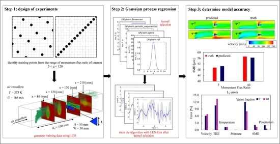
Figure 1 shows the schematic of the framework. It consists of three steps: (1) identification and generation of training and testing databases—these databases established using LES will be referred to as truth model hereafter; (2) training of the GPML algorithm using the training database; and (3) error quantification based on comparison of GPML predicted results with the truth model under test conditions. It should be noted that the testing database was not used for training, instead, it was used exclusively to test the accuracy of the GPML predictions at test points. Furthermore, the framework is agnostic to the source of data—the truth model can also be high-resolution experimental measurements. These three steps are described briefly below:
- Step 1: generation of training (and testing) data
This step involves sampling the design space using a single variable worst-case scenario Latin Hypercube Sampling (LHS) technique [39,40] in combination with knowledge of physical processes dominating the physics under consideration. Since training datasets are expensive to generate (both computationally and experimentally), one of the goals was to use a minimum set of data points while maximizing accuracy, which was one of the reasons for choosing GPR which is known to do well with sparse data. Once a set of conditions for training data points was selected, LES-based calculations were conducted under each of those conditions. The configuration chosen here was representative of fuel injected into crossflowing air in a ramjet engine. Some of the relevant non-dimensional numbers for the present flow were the gas Reynolds number Reg, Reynolds number based on jet diameter Red, the liquid Weber number, Weg = ρgURd/σ the gas Weber number, and momentum flux ratio q. The importance of some of these non-dimensional numbers for the present flow configuration is discussed in [32]. While we could have chosen to vary any of these important parameters to demonstrate that our model provides speed up and is accurate for turbulent multiphase flow problems, we chose the momentum flux ratio because it takes into account both the dynamics of the gaseous and liquid phase effects [16]. The penetration depth of the injected fuel depends upon the jet velocity. Momentum flux ratio was, therefore, chosen as a parameter of engineering significance, and the data set was collected at an increasing momentum flux ratio. As shown in our previous paper [17], adding more training points can increase the accuracy of predictions up to a certain extent, after which the accuracy improves at a much lower rate as compared to the decline in speedup with the addition of more points. To maintain a balance between speedup and accuracy, in this manuscript, we deemed a 15% error from truth data as appropriate to achieve two orders of magnitude accuracy over LES calculations. To test the accuracy of the trained algorithm, a few testing points were also determined and corresponding data were generated using LES.
- Step 2: Gaussian process regression
This step involves selecting a kernel function to model the covariance of each of flow quantities of interest—velocities, turbulent kinetic energy (TKE), pressure, temperature, vapor fractions, liquid jet penetration depth, and the Sauter mean diameter (SMD) of the droplet size distribution. In general, selecting kernel shapes is the most critical step in GP based prediction techniques. For the current work, kernel functions were selected based on the behaviors of the corresponding flow variables in the most dynamic regions of the flow domain, such as the wakes downstream of the liquid jet and the bluff body to ensure that maximum variation across the data points was captured. It should be noted that the “most” dynamic regions that we referred to in the previous sentence can be different for different variables. In addition to regions of the most action, since our goal was to have one kernel function to model the behaviors of a given flow variables at every point in the flow, the additive property of GP kernels facilitates their selection, such that different terms can dominate the model at different spatial locations. Another strategy can be to divide the domain into multiple zones based on some criteria (physics-based preferred), and then select different kernels for different zones. After selecting a kernel function, the entire flowfield is subjected to the GPR-based training process.
- Step 3: error quantification
In this step, the accuracy of the machine learning algorithm was established using the L1 error norm. This was conducted by predicting the gaseous and spray dynamics under testing conditions established in step 1 using the GPML algorithm trained in step 2 and comparing the results with the truth model. For clarity, the predictions from the trained machine learning algorithm will be referred to as predictions, and the results from LES calculations will be referred to as the truth model for the rest of this manuscript.
3. Theoretical Formulations and Governing Equations for the Truth Model
The truth model is based on a compressible Eulerian–Lagrangian LES framework. The next few subsections briefly describe the governing equations and the numerical methodology for the gaseous and the liquid phases. For a detailed description, the reader is referred to our previous publications [32,33].
3.1. Governing Equations for the Gaseous Phase
The governing equations were formulated and solved to satisfy the conservation of mass, momentum, energy, and species transport in Cartesian coordinates. Source terms appeared due to interaction with the dispersed phase droplets. Large eddy simulation (LES) technique was used to achieve turbulence closure. The Favre averaged equations are given by:
Spatially filtered variables, Favre-averaged variables, viscous stress tensor, and heat flux vector are denoted as: , , , , respectively. refers to the mass fraction of the kth species. The species diffusion flux is denoted by . The sub-grid scale (SGS) stresses term , SGS energy fluxes term and SGS species fluxes result from filtering these convective terms. The SGS viscous work term, , comes from correlations of the velocity field with the viscous stress tensor, and the SGS species diffusive fluxes term, , comes from correlations of the velocity field with the species mass fractions with the diffusion velocities. The resolved-scale species mass production rate, , is also unclosed. These SGS terms are closed using the algebraic version of the Smagorinsky model, as given by Erlebacher, et al. [6]. The details of the model are discussed elsewhere [41]. The terms , , , and represent the interphase exchange of mass, momentum, energy, and species between the gas phase and the spray. The coupling between the two phases is described in Section 3.2.2.
3.2. Dispersed Phase Modeling
A Lagrangian approach was used to model the droplets and their kinematics. The source terms associated with the transfer of mass, momentum, and energy between the dispersed and continuous phase were distributed across the diameter of the droplet. In this way, the present method accounted for the finite size of the droplets; details of this method can be found elsewhere [33]. Since tracking every droplet is a computationally expensive process, multiple droplets of similar size, location, velocity, and temperature were grouped together and treated as a parcel—this is known as the blob approach in the literature. The motion of particles was determined as Newton’s second law of motion as follows:
where is the instantaneous particle location, and is the droplet mass. Only the force arising from skin friction and form drag was considered, after neglecting contributions from virtual mass, buoyancy, Basset forces, gravity, and lift.
and are the particle diameter and velocity relative to the surrounding carrier fluid, respectively. Droplet mass transfer due to vaporization is governed by the droplet continuity equation, as shown below:
where md is the mass of the droplet, which is given by , and is the net mass transfer rate of droplet mass due to vaporization, which is expressed as:
is the Reynolds number for a droplet at rest. The energy equation was solved to calculate the droplet heat transfer. This accounted for convective heat transfer between the droplet and surrounding air as well as latent heat of vaporization. Temperature was assumed to be uniform throughout the droplet. The equation governing the droplet temperature is given by:
where is the convective thermal energy transfer rate, is liquid heat capacity, is the heat transfer coefficient, and is the latent heat of vaporization.
3.2.1. Spray Closure Modeling
The hydrodynamic stability analysis developed by Reitz [42] was implemented to model the jet injection and atomization process. Here, the liquid jet was injected as blobs of diameter equal to injector exit diameter do, i.e., dint = do. The number of blobs injected per unit time was based on the injector mass flow rate. Each blob was injected at velocity Uo and at a spray angle θ, which was assumed to be uniformly distributed between 0 and Φ, with:
where A1 has a value of 0.188 for a sharp entrance nozzle with a length to diameter ratio of 5. The theory of Kelvin–Helmholtz (K-H) instability in jets was used to determine the frequency associated with the fastest growing instability wave, , and the corresponding wavelength, λ. These values were determined by performing a curve-fit solution of the linearized hydrodynamic equations, and presented in non-dimensional quantities which are specified by:
where is the Ohnesorge number, is the liquid Weber number, is the gas Weber number, and is the Taylor number. The variable a is the blob/parent droplet radius. The subscripts l and g denote the liquid and gas phases, respectively. The breakup of liquid droplets moving in surrounding air was assumed to be caused by instability waves induced by the deceleration of the droplets caused by aerodynamic drag. The breakup of the droplets was modeled such that their sizes were proportional to the wavelength of the fastest growing instability wave droplets, and is given by:
where B0 is constant and equals 0.61. Once the parent droplet broke up, its mass was assigned to child droplets, and then these droplets were tracked. The rate of change of drop radius in a parent parcel was assumed to obey the following equation:
where , with B1 being a breakup time constant, and is set to a value of 1.73 as per the recommendation made by Liu et al. [43]. Secondary atomization was modeled by using The Taylor analogy breakup (TAB) model [44], and the impingement of droplets on solid surfaces (walls) was treated using the model developed by Mundo et al. [45]. More information about multiphase flow modeling can be found in [33].
3.2.2. Coupling between Dispersed and Carrier Phase
Coupling between the dispersed phase and gas phase was accounted for by calculating the interphase exchange between the dispersed phase and carrier air. The source terms that accounted for this exchange were computed as follows:
where the summation index m accounts for all the droplet parcels that cross a given computational cell volume.
Governing equations for the gaseous phase was solved using the finite volume method employed on a structured grid. The spatial discretization method used was a second-order accurate central-difference scheme used in generalized coordinates. A fourth-order matrix dissipation scheme with a total variation-diminishing method was applied to ensure numerical stability by preventing numerical oscillations in locations where steep gradients may be present. Temporal discretization was performed using the fourth order Runge–Kutta method. Multi-block domain decomposition was used to implement parallel computations, with message passing interface at the domain interface. Further details of these techniques can be found elsewhere [1,33,41].
4. Error Quantification and Speedup
Errors were estimated to quantify the degree of accuracy achieved with the surrogate model when compared with the original simulation. The error between the predicted quantity and truth model was estimated for each grid location and averaged for all grid points to obtain the average L1 error defined by:
The speedup afforded by the surrogate model was measured as the ratio of CPU hours needed by the truth model and the GPML algorithm for the test condition under consideration. The number of processors required and the actual computational time in hours were combined to arrive at a CPU hours metric as shown below:
The speedup factor could then be estimated by:
5. Results and Discussion
The results are organized into four subsections. In the next subsection, comparisons between the LES results and experimental measurements are presented to establish the credibility of the truth model. A brief description of flow features associated with vaporizing liquid jet in crossflow is also provided. This is followed by a subsection describing the selection of training points. Results for the gaseous and liquid phases predicted by GPML are discussed in Section 5.3 and Section 5.4, respectively.
5.1. Experimental Validation of the Truth Model
The theoretical framework presented above is validated with experimental measurements made by Stenzler et al. [21]. The results were compared for both vaporizing and non-vaporizing cases. Figure 2 shows the schematic of the computational setup. Table 1 lists all the operating conditions, the physical properties of air as well as the liquid jet, and all relevant non-dimensional numbers used here.
A total of 5.1 × 10⁶ grid points were used to mesh the entire computational domain. Figure 3 shows a perspective view of the multi-block grid that was used. However, only every 5th grid volume is retained in the figure. The grid was particularly well refined close to the jet injection location so that the unsteady wake shed downstream may be well resolved. The smallest grid size was 0.02 and 0.01 mm in the x and z directions, respectively. At least 10 grid points were used to resolve the diameter of the jet. The dense grid was retained up to 12 injector diameters (3 mm) downstream of the injector location, and 1.6 diameters (0.4 mm) in the z direction. The grid was then gradually stretched before refining it once again, close to wall surfaces. The current grid resolved over 80% of the turbulent kinetic energy (TKE) for a jet Reynolds number of 2059. To account for inflow turbulence reported in experiments, a precursor turbulent channel flow simulation was first conducted at the appropriate Reynolds number to generate the corresponding turbulent flowfield. The instantaneous flowfield data obtained from this turbulent channel flow were then fed into the computational domain for the validation cases.
Figure 4a,b show the comparison of the liquid jet penetration and its trajectory obtained from the present study. Results were compared with correlations developed by Stenzler et al. [21], based on experimental measurements. The correlation curves represent the upper edge of the jet core. The outer edge of the jet is based on experimental imaging and is the locus of points where the droplet/jet was observed at the furthest point in the direction perpendicular to the air flow. The results are shown for the non-vaporizing and vaporizing cases, respectively, showing good agreement with the correlation curves.
A quantitative comparison was made by showing droplet size distributions in Figure 5a–d, where the evolution of the Sauter mean diameter (SMD) with distance is shown by presenting the SMD contours at locations 1,9,18, and 25.4 mm downstream of the jet. The results shown here are for the non-vaporizing case. The gradual expansion of the jet core is evident from the figures. Upon further inspection, it is seen that the largest droplets (55–65 µm) were found close to the upper edge of the jet core, while the midsized droplets were concentrated in the jet core. Relatively smaller droplets were distributed close to the bottom. As shown in Figure 6, the SMD distribution compares well with experimental measurements made by Stenzler et al. [21], thus confirming our observations. The comparison was made for the location that was 25.4 mm downstream of the injector. While the trends were generally in agreement, the experimental measurements show that there was a small fraction of larger sized droplets at the center of the core as compared to the present simulations that predict these droplets to be presented mostly close to the upper edge of the jet core.
It should be noted that the wake behind the liquid jet needs to be captured with a denser grid to ensure the accuracy of both the gaseous and liquid spray fields and for reliable droplet statistics. The unsteady wake was resolved using the finite-sized formulation of the two-way coupling developed by Khare et al. [33]. Figure 7 shows the instantaneous contour of vorticity magnitude immediately downstream of the jet wake. An intense exchange of momentum between the liquid jet and inflowing air gave rise to turbulence unsteady fluctuations in the wake of the jet. These turbulent fluctuations constituted shed wake vortices, counter-rotating vortex pairs, and vortices generated in the boundary layer close to the bottom wall. Furthermore, to quantitatively identify the turbulent wake, time-series data for velocity fluctuations were collected at a probe located 2 mm immediately downstream of the liquid injection location. Figure 8 shows the spectra obtained by taking the fast Fourier transform (FFT) of the velocity fluctuations, which follows the −5/3 law of the Kolmogorov–Obukhov theory for turbulent flows.
5.2. Configuration and Operating Conditions for Training Dataset
A more realistic configuration relevant to ramjet and afterburner engines was used to demonstrate that our machine learning algorithm can be employed for design space exploration parametrized by the momentum flux ratio that ranges from 5 to 120; all other relevant non-dimensional numbers including the Reynolds and Weber numbers are approximately constant. Figure 9 shows a schematic of the configuration—the major difference from the validation case was the presence of a triangular bluff body downstream of the liquid injection location. The flow configuration consisted of liquid water injected into cross-flowing air at atmospheric pressure but at an elevated temperature of 600 K. The computational domain consisted of a 248.7 × 50 × 50 mm3 domain. The liquid jet was located at Lj = 40 mm from the leading edge of the domain, and the v-gutter was located further downstream at a separation of Ls = 100 mm. The v-gutter is an equilateral triangle with a side of length of L = 10 mm. Airflow was kept constant at a flow velocity Ug of 141.6 m/s, and the momentum flux ratio was varied between 5 and 120 by increasing the liquid jet injection velocity Ul from 7.04 to 37.31 m/s. It should be noted that this led to an increase in the Weber number by 6%. Quantitative comparisons between the GPML predictions and truth models were made at four planes corresponding to x = 80, 120, 170, and 210 mm from the inlet. Knowledge of the behaviors of flow quantities such as velocities, pressure, temperature, vapor-fraction, and turbulent kinetic energy (TKE) with increasing momentum flux ratio was utilized for identifying a set of training and testing points. Amounts of 420, 198, and 101 grid points were used in the x, y, and z-directions, respectively, with 240 grid points upstream of the bluff body and 180 downstream of it. This results in a total of 8 million points to mesh the computational grid.
Figure 10 shows the spray fields obtained from LES-based calculations at three representative momentum flux ratios of q = 5, 30, and 120. At the value of q = 5, the jet did not have sufficient momentum to penetrate deep into the test section, and the droplets were concentrated closer to the bottom wall, well below the v-gutter. At q = 30, the core of the spray field penetrated deeper and was within the vicinity of the v-gutter. With a further increase in momentum flux ratio, for q = 120, the injected jet impinged on the upper wall and most of the droplets were concentrated close to the upper wall.
The design of experiments based on LHS worst-case scenario and the domain knowledge of jet behavior facilitated the selection of training data points. Both the extreme cases of q = 5, 120, and an intermediate point q = 10 where the jet impinged on the v-gutter, were included in the training dataset of the GPML algorithm. Table 2 lists the points selected for training the surrogate model. Once the algorithm was trained, several operating points in the momentum flux parameter space were chosen at random to test its accuracy; these testing points are listed in Table 3.
As mentioned before, to quantify the accuracy, we compared the GPML predictions at the mid-plane of the computational domain for time-average streamwise velocity, TKE, pressure, temperature, the mass fraction of vaporized water, and temperature are reported at four select streamwise stations located at 80, 120, 170, and 210 mm from the inlet plane under test conditions listed shown in Figure 9. The first station was in the wake of the liquid jet, and the second one further downstream before the v-gutter. The next two locations were chosen downstream of the v-gutter, with one within the wake of the v-gutter and the other one further downstream of the wake.
Once trained, the machine algorithm was capable of emulating any momentum flux ratio within the training bounds of q = 5 and 120. In the current manuscript, we show the comparison of the predictions by the trained algorithm with truth data for 2 testing points identified by q = 7 and 40.
5.3. Results of Machine Emulation
In the next few subsections, we will discuss how the statistically stationary time-averaged flow variables predicted by the trained GPML algorithm compared with the truth data obtained using LES at test points of q = 7 and 40 at the mid-plane followed by the profiles of flow variable at the previously mentioned streamwise locations. The errors will be quantified by L1 norms. While a brief description of the physical processes is provided as we discuss each flow variable, readers are referred to our previous work that discusses the effect of the momentum flux ratio on the detailed flow physics [32]. It should be noted that the accuracy of the GPML algorithm is directly proportional to the accuracy of the training data, which in this case is the results from LES calculations.
5.3.1. Velocity Magnitude
Figure 11a shows the mid-plane contours of velocity magnitude predicted by the GPML algorithm (left) and truth data (right) for test conditions of q = 7 and 40, showing excellent qualitative agreement. To further quantify differences, Figure 11b shows a comparison of the velocity profiles at x = 80, 120, 170, and 210 mm—the solid lines represent the truth model and the dashed lines show machine learning emulations. The wakes downstream of the liquid jet and the v-gutter and the flow acceleration on the top and bottom of the v-gutter were accurately captured by the GPML predictions, as shown in Figure 11b at all four locations. To quantify the differences, the L1 norm was calculated for the entire flow domain. The machine learning predictions for q = 7 differed from the truth model by 6.05% and for q = 40 by 6.76%. The kernel function used for machine emulation of velocity magnitude is given by:
5.3.2. Turbulent Kinetic Energy
To demonstrate that our algorithm can predict second-order turbulence statistics, TKE was also predicted and compared with the truth data at test points, shown in Figure 12a,b. TKE contours provided an estimate of the level of turbulence at different locations in the flow domain. Momentum transfer from the gas phase to the dispersed liquid phase had a significant effect on TKE. Velocity fluctuations increased in the immediate wake of the jet but were still a few orders of magnitude lower than that of turbulent fluctuations in the unsteady wake of the v-gutter. As the flow accelerated past the bluff-body, these fluctuations were intensified resulting in higher TKE downstream of the v-gutter—turbulent fluctuations were the strongest at this location. This phenomenon can be observed in the TKE plots in Figure 12b, at x = 170 mm for both cases. For q = 40, the intensity of the turbulent fluctuations was reduced due to a higher transfer of momentum from the gas phase to the liquid phase. The unsteady wake was smaller in size when compared to the q = 7 case as the injected liquid phase damped some of these fluctuations, which resulted in reduced freestream velocity and turbulence intensity. All these observations were effectively captured by the GPML predictions not only qualitatively but also quantitatively presented in Figure 12b, where the solid lines represent the truth model and the dashed lines show machine learning emulations. The error quantified by the L1 norm for the entire flow domain was 10.47% for q = 7 and 13.26% for q = 40. The kernel function used for machine emulation of TKE is given by:
5.3.3. Pressure and Temperature
Figure 13a,b show a comparison of pressure fields predicted by the GPML algorithm and truth data from LES showing excellent agreement for q = 7 and 40, evidenced by the L1 error of 0.05% for q = 7 and 0.07% for q = 40.
Figure 14a shows the temperature contours for both cases. For q = 7, since most of the injected liquid was in the lower half of the domain, a significant drop in temperature was observed in the jet wake—energy from the gas was used to vaporize the liquid jet. Similar trends were observed for q = 40, except that the lower temperature zone encompassed a considerably larger region of the domain in the y-direction because of the higher momentum carried by the liquid. As shown in Figure 14b, all these trends were effectively captured quantitatively by the GPML algorithm. The L1 error for temperature over the entire domain was found to be 1.18% for both q = 7 and q = 40. The kernel function used for machine emulation of pressures and temperatures is given by:
5.3.4. Liquid-Vapor Fraction
Heat transfer from the hot gas to the cooler water resulted in the vaporization of the liquid phase. Therefore, the variation of the liquid-vapor fraction closely corresponded to the locations of lower temperature regions discussed in the previous subsection. These are shown qualitatively as vapor fraction contours in Figure 15a and quantitatively at the four stations in the streamwise direction in Figure 15b. The L1 error was calculated to quantify the accuracy of the GPML predictions as compared to the truth model; L1 errors were found to be 11.91% for q = 7 and 7.99% for q = 40. The kernel function used for machine emulation of the liquid-vapor fraction is given by:
5.3.5. Sauter Mean Diameter (SMD) and Jet Penetration Depth
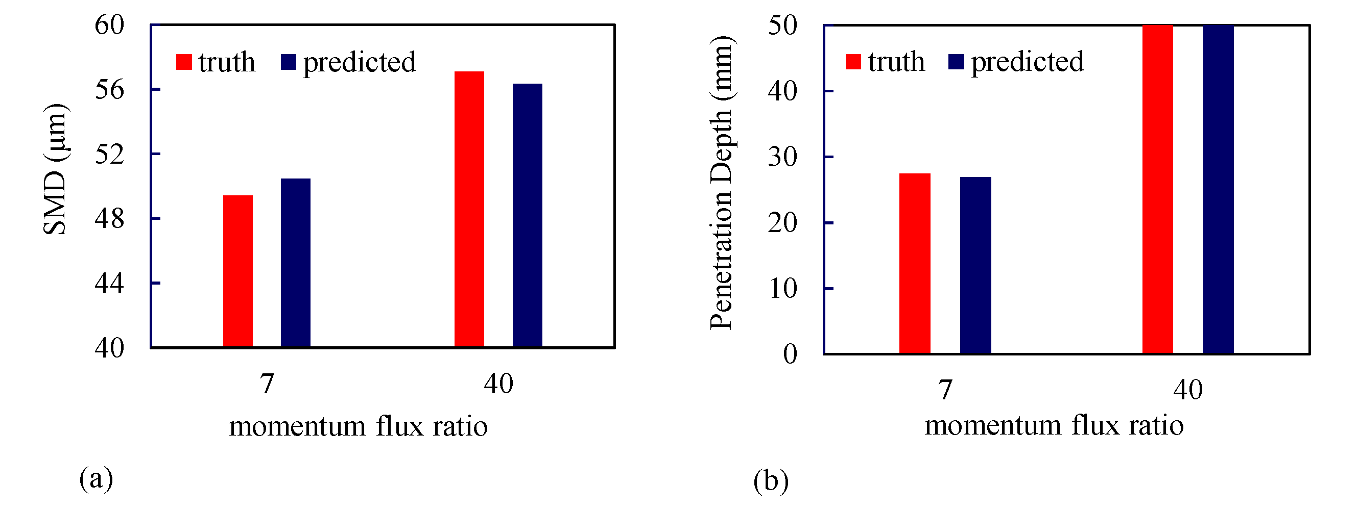
Figure 16a,b, respectively show a comparison of the Sauter mean diameter and liquid jet penetration depth predicted by the GPML algorithm and the truth model for test points corresponding to q = 7, and 40. The L1 error for SMD was 2.11% for q = 7 and 1.30% for q = 40, and for the liquid jet penetration depth was 2.03% for q = 7 and 0.55% for q = 40. The kernel function used for machine emulation of SMD and jet penetration depth is given by:
5.4. Speedup
The speedup was calculated as follows:
The total CPU hours required by the LES-based calculations to reach a statistically stationary state and for collecting reliable higher-order statistics for the test points were approximately 27,360 h. A total of 21 h on 20 cores were needed to train the GPML algorithm, resulting in a total of 420 CPU hours. Thus, the speedup was approximately 65.
6. Summary
A data-driven surrogate model was successfully built by extending a previously developed Gaussian process-based algorithm to accommodate turbulent multiphase flows. The surrogate model was applied to liquid jet injection in turbulent air crossflow, a canonical configuration that represents fuel injection in afterburner and ramjet engines. The algorithm was trained using data generated by an Eulerian–Lagrangian-based LES framework. Before training the machine learning framework, the LES model was validated against measurements for both non-vaporizing and vaporizing sprays. The training points were identified by the momentum flux ratio, which varied between 5 and 120. The Gaussian process-based machine learning algorithm was then trained using the LES data at momentum flux ratios determined based on a design of experiments study. To test the accuracy of the surrogate model, emulated results at representative test points of q = 7 and 40, were compared against LES data in the mid-plane of the geometry. The model predicted spatial variations of the velocity magnitude, pressure, temperature, vapor fraction, TKE, liquid penetration, and SMD with reasonable accuracy (varying between 0.05 and 13.5%). Corresponding to these emulated results, a speedup of 65 was achieved. Based on these observations, we hope that this methodology can be leveraged (and further improved) for conducting large scale parameter sweeps and uncertainty quantification studies for the design of devices based on turbulent multiphase flows.
The algorithm and methodology developed in this study can be applied to other fields of science and engineering for steady-state or statistically stationary flows. Except for selecting a kernel function to capture the signal variation across training datasets, the methodology remains unchanged. For spatiotemporally evolving flows, it is recommended to reduce the dimensionality, especially in the time domain, using some kind of modal decomposition technique for computational efficiency and improvements in speedup. Application of the algorithm used in this paper to spatiotemporally varying flows has been successfully demonstrated in our previous work [17]. While this paper represents the first effort in predicting turbulent multiphase flows using machine learning techniques, it is just the first step towards the development of a comprehensive framework that can be used for engineering design. The next step is to develop machine learning algorithms capable of predicting fluid dynamic behaviors when multiple independent parameters are varied simultaneously, which is a closer representation of the design space that is encountered in the preliminary and detailed design stages.
Author Contributions
Conceptualization, P.K.; methodology, P.K.; software, H.G., M.K., and P.K.; validation, H.G. and M.K.; formal analysis, H.G. and M.K.; investigation, H.G. and M.K.; resources, P.K.; data curation, H.G. and M.K.; writing—original draft preparation, H.G. and M.K.; writing—review and editing, P.K.; visualization, H.G., M.K., and P.K.; supervision, P.K.; project administration, P.K.; funding acquisition, P.K. All authors have read and agreed to the published version of the manuscript.
Funding
This research received no external funding.
Acknowledgments
The computational resources used for this research were provided in part through research cyberinfrastructure resources and services provided by the Advanced Research Computing (ARC) center at the University of Cincinnati, and in part by and the DoD High Performance Computing Modernization Program (HPCMP) subproject number, ARLAP44862H70.
Conflicts of Interest
The authors declare no conflict of interest.
References
- Li, H.-G.; Khare, P.; Sung, H.-G.; Yang, V. A Large-Eddy-Simulation study of combustion dynamics of Bluff-Body stabilized flames. Combust. Sci. Technol. 2016, 188, 924–952. [Google Scholar] [CrossRef]
- Yoo, Y.-L.; Han, D.-H.; Hong, J.-S.; Sung, H.-G. A large eddy simulation of the breakup and atomization of a liquid jet into a cross turbulent flow at various spray conditions. Int. J. Heat Mass Transf. 2017, 112, 97–112. [Google Scholar] [CrossRef]
- Jiang, X.; Siamas, G.A.; Jagus, K.; Karayiannis, T.G. Physical modelling and advanced simulations of gas-liquid two-phase jet flows in atomization and sprays. Prog. Energy Combust. Sci. 2010, 36, 131–167. [Google Scholar] [CrossRef]
- Moin, P.; Apte, S.V. Large-eddy simulation of realistic gas turbine combustors. AIAA J. 2006, 44, 698–708. [Google Scholar] [CrossRef]
- Madabhushi, R.K. A Model for Numerical Simulation of Breakup of a Liquid Jet in Crossflow. At. Sprays 2003, 13, 413–424. [Google Scholar] [CrossRef]
- Erlebacher, G.; Hussaini, M.Y.; Speziale, C.G.; Zang, T.A. Toward the large-eddy simulations of compressible turbulent flows. J. Fluid Mech. 1992, 238, 155–185. [Google Scholar] [CrossRef] [Green Version]
- Broumand, M.; Birouk, M. Liquid jet in a subsonic gaseous crossflow: Recent progress and remaining challenges. Prog. Energy Combust. Sci. 2016, 57, 1–29. [Google Scholar] [CrossRef]
- Song, J.; Cain, C.C.; Lee, J.G. Liquid Jets in Subsonic Air Crossflow at Elevated Pressure. J. Eng. Gas Turbines Power 2014, 137. [Google Scholar] [CrossRef]
- Lee, K.; Aalburg, C.; Diez, F.J.; Faeth, G.M.; Sallam, K.A. Primary Breakup of Turbulent Round Liquid Jets in Uniform Crossflows. AIAA J. 2007, 45, 1907–1916. [Google Scholar] [CrossRef]
- Vich, G.; Ledoux, M. Investigation of a liquid jet in a subsonic cross-flow. Int. J. Fluid Mech. Res. 1997, 24, 1–12. [Google Scholar] [CrossRef]
- Kihm, K.D.; Lyn, G.M.; Son, S.Y. Atomization of Cross-Injecting Sprays Into Convective Air Stream. At. Sprays 1995, 5, 417–433. [Google Scholar] [CrossRef]
- Zang, Y.; Street, R.L.; Koseff, J.R. A dynamic mixed subgrid—Scale model and its application to turbulent recirculating flows. Phys. Fluids A Fluid Dyn. 1993, 5, 3186–3196. [Google Scholar] [CrossRef]
- Birouk, M.; Lekic, N. Liquid Jet Breakup in Quiescent Atmosphere: A Review. At. Sprays 2009, 19, 501–528. [Google Scholar] [CrossRef]
- Sallam, K.A.; Dai, Z.; Faeth, G.M. Liquid breakup at the surface of turbulent round liquid jets in still gases. Int. J. Multiph. Flow 2002, 28, 427–449. [Google Scholar] [CrossRef]
- Mazallon, J.; Dai, Z.; Faeth, G.M. Primary breakup of nonturbulent round liquid jets in gas crossflows. At. Sprays 1999, 9, 291–311. [Google Scholar] [CrossRef]
- Wu, P.-K.; Kirkendall, K.A.; Fuller, R.P.; Nejad, A.S. Breakup Processes of Liquid Jets in Subsonic Crossflows. J. Propuls. Power 1997, 13, 64–73. [Google Scholar] [CrossRef]
- Ganti, H.; Khare, P. Data-Driven Surrogate Modeling of Multiphase Flows Using Machine Learning Techniques. Comput. Fluids 2020, 211, 104626. [Google Scholar] [CrossRef]
- Wu, P.-K.; Faeth, G.M. Aerodynamic Effects on Primary Breakup of Turbulent Liquids. At. Sprays 1993, 3, 265–289. [Google Scholar] [CrossRef] [Green Version]
- Amighi, A.; Ashgriz, N. Global Droplet Size in Liquid Jet in a High-Temperature and High-Pressure Crossflow. AIAA J. 2019, 57, 1260–1274. [Google Scholar] [CrossRef]
- Oh, J.; Lee, J.G.; Lee, W. Vaporization of a liquid hexanes jet in cross flow. Int. J. Multiph. Flow 2013, 57, 151–158. [Google Scholar] [CrossRef]
- Stenzler, J.N.; Lee, J.G.; Santavicca, D.A.; Lee, W. Penetration of liquid jets in a cross-flow. At. Sprays 2006, 16, 887–906. [Google Scholar] [CrossRef]
- Rachner, M.; Julian, B.; Christoph, H.; Thomas, D. Modelling of the atomization of a plain liquid fuel jet in crossflow at gas turbine conditions. Aerosp. Sci. Technol. 2002, 6, 495–506. [Google Scholar] [CrossRef]
- Wang, Q.; Hesthaven, J.S.; Ray, D. Non-intrusive reduced order modeling of unsteady flows using artificial neural networks with application to a combustion problem. J. Comput. Phys. 2019, 384, 289–307. [Google Scholar] [CrossRef] [Green Version]
- Takbiri-Borujeni, A.; Kazemi, H.; Nasrabadi, N. A data-driven proxy to Stoke’s flow in porous media. arXiv 2019, arXiv:1905.06327. [Google Scholar]
- Yeh, S.-T.; Wang, X.; Sung, C.-L.; Mak, S.; Chang, Y.-H.; Zhang, L.; Wu, C.F.J.; Yang, V. Common Proper Orthogonal Decomposition-Based Spatiotemporal Emulator for Design Exploration. AIAA J. 2018, 56, 2429–2442. [Google Scholar] [CrossRef] [Green Version]
- Moiz, A.A.; Pal, P.; Probst, D.; Pei, Y.; Zhang, Y.; Som, S.; Kodavasal, J.A. A Machine Learning—Genetic Algorithm (ML-GA) Approach for Rapid Optimization Using High-Performance Computing. SAE Int. J. Commer. Veh. 2018, 11, 291–306. [Google Scholar] [CrossRef]
- Raissi, M.; Perdikaris, P.; Karniadakis, G.E. Physics Informed Deep Learning (Part II): Data-driven Discovery of Nonlinear Partial Differential Equations. arXiv 2017, arXiv:1711.10561. [Google Scholar]
- Bai, Z.; Brunton, S.L.; Brunton, B.W.; Kutz, J.N.; Kaiser, E.; Spohn, A.; Noack, B.R. Data-Driven Methods in Fluid Dynamics: Sparse Classification from Experimental Data. In Whither Turbulence and Big Data in the 21st Century; Pollard, A., Castillo, L., Danaila, L., Glauser, M., Eds.; Springer International Publishing: Cham, Switzerland, 2017; pp. 323–342. [Google Scholar]
- Brunton, S.; Proctor, J.L.; Kutz, J.N. Discovering governing equations from data by sparse identification of nonlinear dynamical systems. Proc. Natl. Acad. Sci. USA 2016, 113, 3932–3937. [Google Scholar] [CrossRef] [Green Version]
- Moonen, P.; Allegrini, J. Employing statistical model emulation as a surrogate for CFD. Environ. Model. Softw. 2015, 72, 77–91. [Google Scholar] [CrossRef]
- Bright, I.; Lin, G.; Kutz, J.N. Compressive sensing based machine learning strategy for characterizing the flow around a cylinder with limited pressure measurements. Phys. Fluids 2013, 25. [Google Scholar] [CrossRef]
- Kamin, M.; Khare, P. Liquid jet in crossflow: Effect of momentum flux ratio on spray and vaporization characteristics. In Proceedings of the ASME Turbo Expo 2019: Turbomachinery Technical Conference and Exposition, Phoenix, AZ, USA, 17–21 June 2019. [Google Scholar]
- Khare, P.; Wang, S.; Yang, V. Modeling of finite-size droplets and particles in multiphase flows. Chin. J. Aeronaut. 2015, 28, 974–982. [Google Scholar] [CrossRef] [Green Version]
- Hadfield, S.; Lawrence, N.D.; Wilkinson, R.; Durrande, N. Gaussian Process Summer School. 2017. Available online: http://gpss.cc/gpss17/ (accessed on 2 September 2020).
- Ebden, M. Gaussian processes: A quick introduction. arXiv 2015, arXiv:1505.02965. [Google Scholar]
- Rasmussen, C.E. Gaussian Processes in Machine Learning; Springer: Berlin/Heidelberg, Germany, 2004; pp. 63–71. [Google Scholar] [CrossRef] [Green Version]
- Chen, Z.; Wang, B. How priors of initial hyperparameters affect Gaussian process regression models. Neurocomputing 2018, 275, 1702–1710. [Google Scholar] [CrossRef] [Green Version]
- GPSS. GPy: A Gaussian Process Framework in Python. 2014. Available online: http://github.com/SheffieldML/GPy (accessed on 2 September 2020).
- Viana, F.A.C. A Tutorial on Latin Hypercube Design of Experiments. Qual. Reliab. Eng. Int. 2016, 32, 1975–1985. [Google Scholar] [CrossRef]
- Shields, M.D.; Zhang, J. The generalization of Latin hypercube sampling. Reliab. Eng. Syst. Saf. 2016, 148, 96–108. [Google Scholar] [CrossRef] [Green Version]
- Oefelein, J.C.; Yang, V. Modeling High-Pressure Mixing and Combustion Processes in Liquid Rocket Engines. J. Propuls. Power 1998, 14, 843–857. [Google Scholar] [CrossRef]
- Reitz, R. Modeling atomization processes in high-pressure vaporizing sprays. At. Spray Technol. 1987, 3, 309–337. [Google Scholar]
- Liu, A.B.; Mather, D.; Reitz, R.D. Modeling the effects of drop drag and breakup on fuel sprays. SAE Trans. 1993, 102, 83–95. [Google Scholar]
- O’Rourke, P.J.; Amsden, A.A. The TAB Method for Numerical Calculation of Spray Droplet Breakup. SAE Technical Paper 872089. 1987. Available online: https://www.sae.org/publications/technical-papers/content/872089/ (accessed on 10 August 2020). [CrossRef] [Green Version]
- Mundo, C.; Sommerfeld, M.; Tropea, C. Droplet-wall collisions: Experimental studies of the deformation and breakup process. Int. J. Multiph. Flow 1995, 21, 151–173. [Google Scholar] [CrossRef]
Figure 1.
Outline of the Gaussian process-based machine learning (GPML) algorithm as applied to statistically stationary vaporizing turbulent liquid jet in crossflow datasets.
Figure 1.
Outline of the Gaussian process-based machine learning (GPML) algorithm as applied to statistically stationary vaporizing turbulent liquid jet in crossflow datasets.
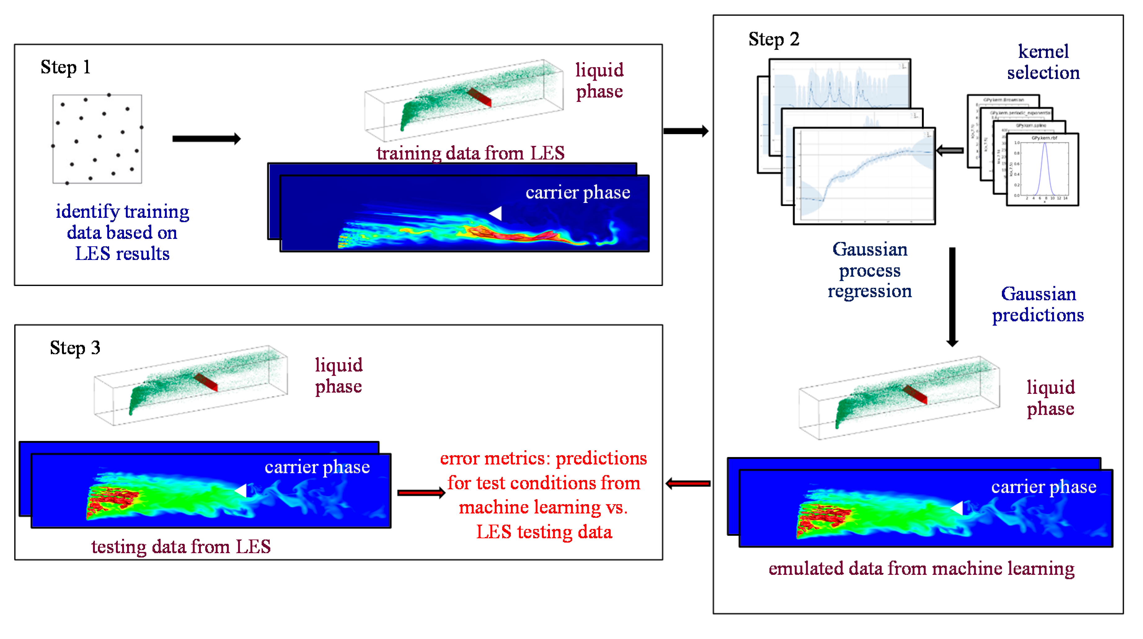
Figure 2.
Schematic of the computational setup for the large eddy simulation (LES) model validation. Two cases were conducted for transverse water injection in air crossflow. For the non-vaporizing case, the air temperature was 300 K and for the vaporizing case, it was 573 K.
Figure 2.
Schematic of the computational setup for the large eddy simulation (LES) model validation. Two cases were conducted for transverse water injection in air crossflow. For the non-vaporizing case, the air temperature was 300 K and for the vaporizing case, it was 573 K.
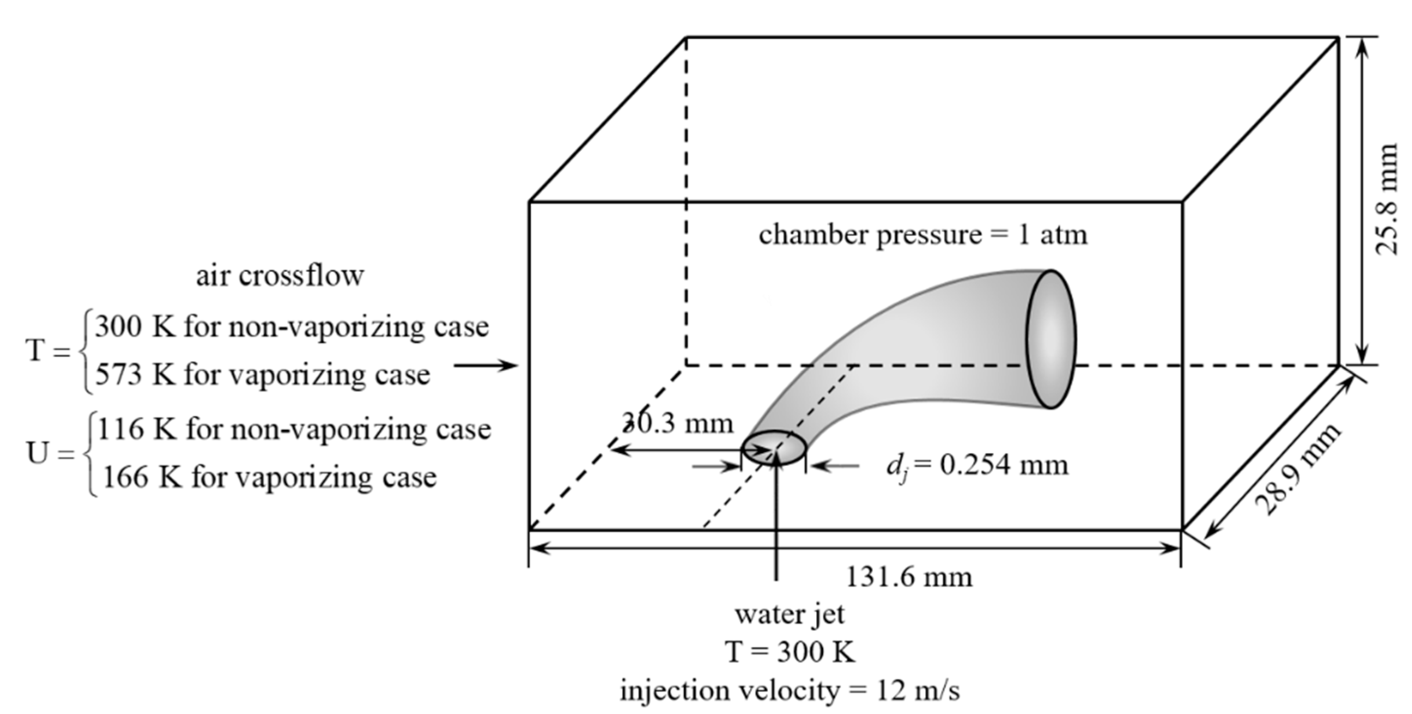
Figure 3.
Grid for the validation cases. A total of 5.1 × 10⁶ grid points were used to mesh the computational domain. This figure shows every 5th grid volume.
Figure 3.
Grid for the validation cases. A total of 5.1 × 10⁶ grid points were used to mesh the computational domain. This figure shows every 5th grid volume.
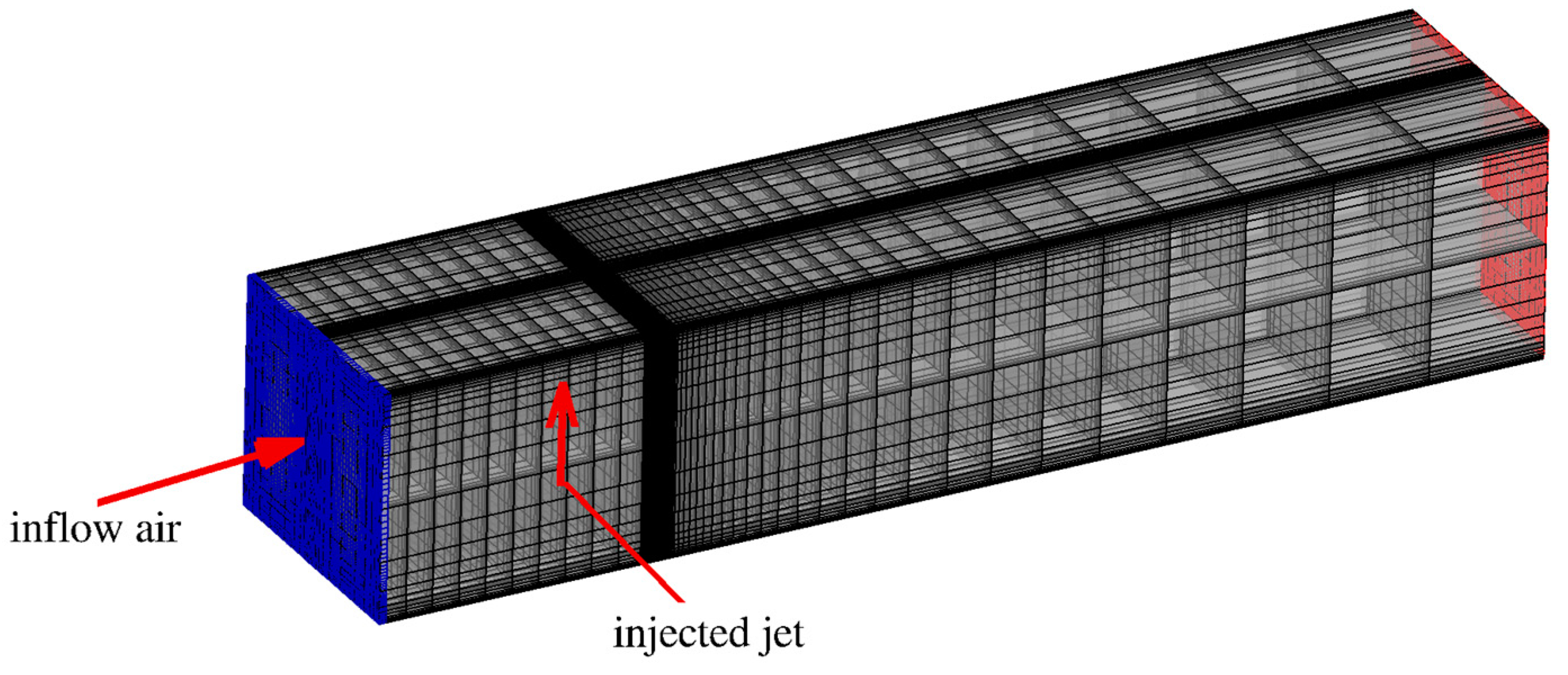
Figure 4.
Comparison of liquid jet penetration with experimental measurements for (a) non-vaporizing and (b) vaporizing cases.
Figure 4.
Comparison of liquid jet penetration with experimental measurements for (a) non-vaporizing and (b) vaporizing cases.
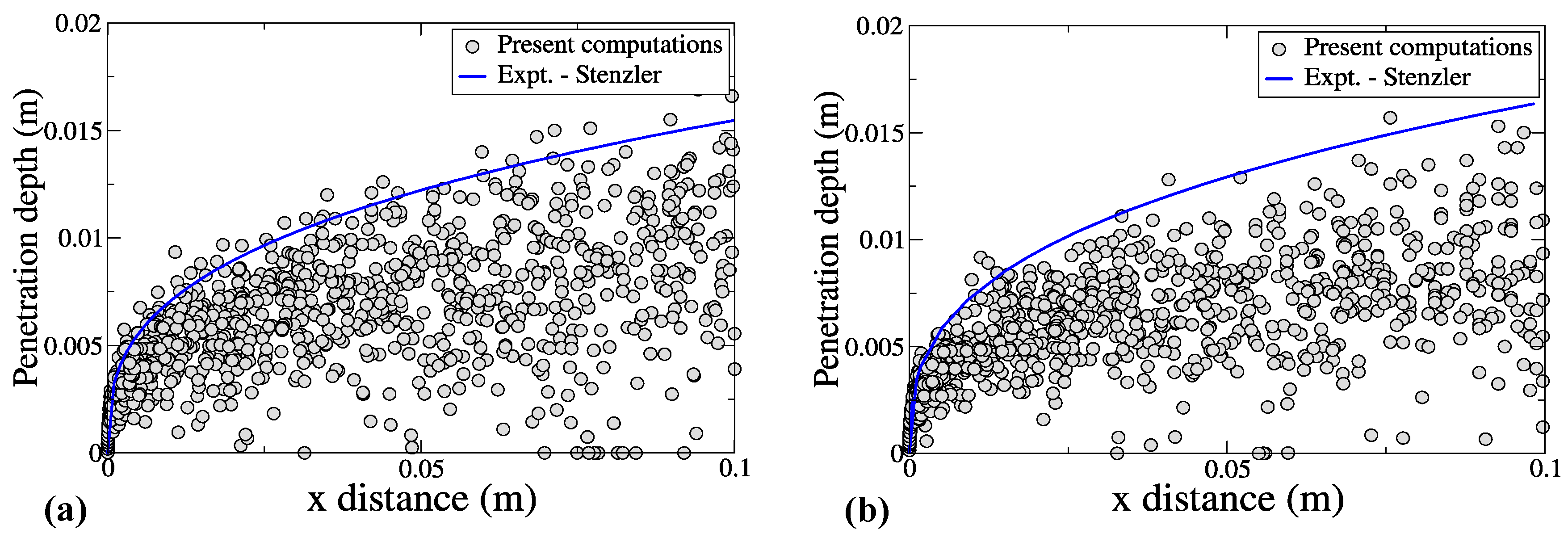
Figure 5.
Sauter mean diameter (SMD) distribution on the y–z plane: progressive streamwise locations showing the development of the spray field at Ta = 300 K at (a) 1 mm, (b) 9 mm, (c) 18 mm, and (d) 25.4 mm downstream of the injection location.
Figure 5.
Sauter mean diameter (SMD) distribution on the y–z plane: progressive streamwise locations showing the development of the spray field at Ta = 300 K at (a) 1 mm, (b) 9 mm, (c) 18 mm, and (d) 25.4 mm downstream of the injection location.

Figure 6.
SMD distribution 25.4 mm downstream of the injector; (a) present calculations and (b) experiments of Stenzler et al. [21].
Figure 6.
SMD distribution 25.4 mm downstream of the injector; (a) present calculations and (b) experiments of Stenzler et al. [21].
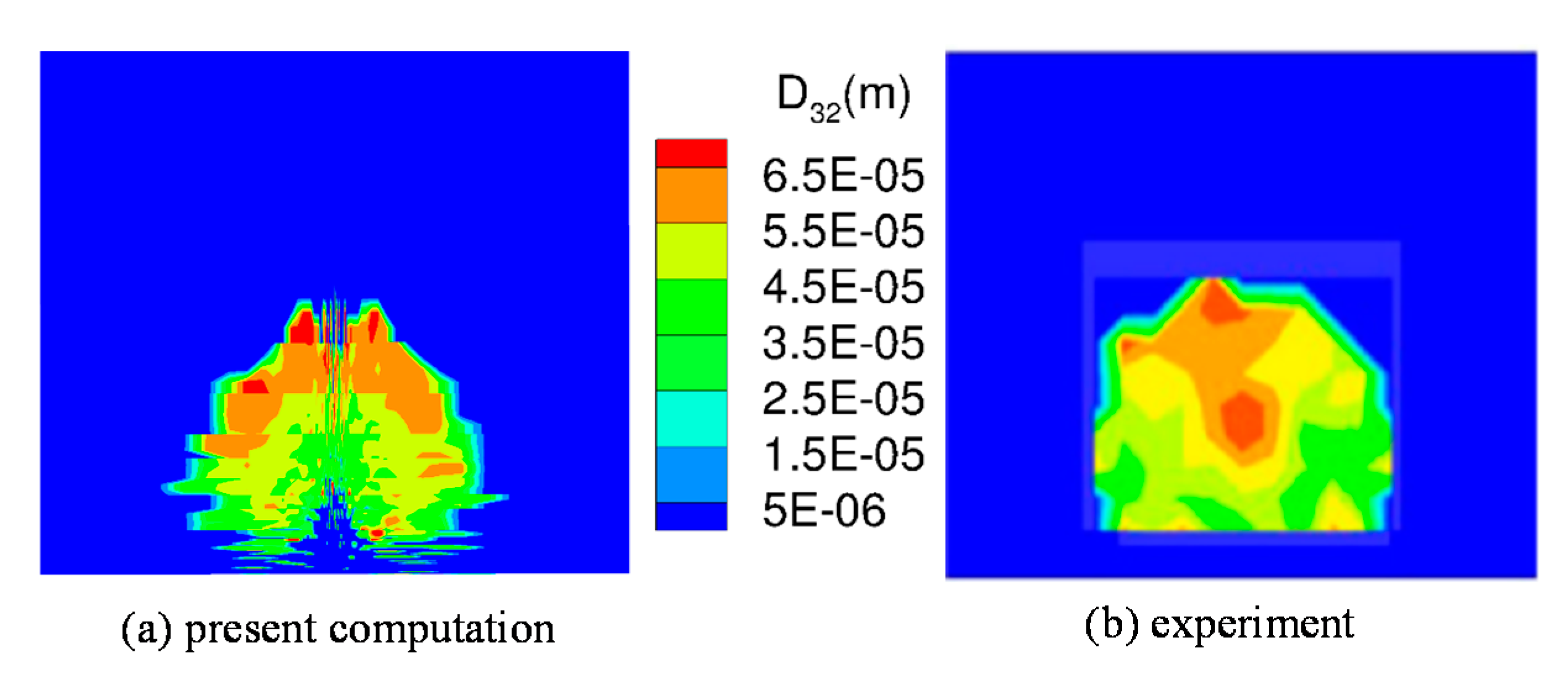
Figure 7.
Instantaneous vorticity contour showing the turbulent wake formation downstream of the liquid jet.
Figure 7.
Instantaneous vorticity contour showing the turbulent wake formation downstream of the liquid jet.

Figure 8.
Turbulence spectra 2 mm downstream of the injector showing the −5/3 slope.
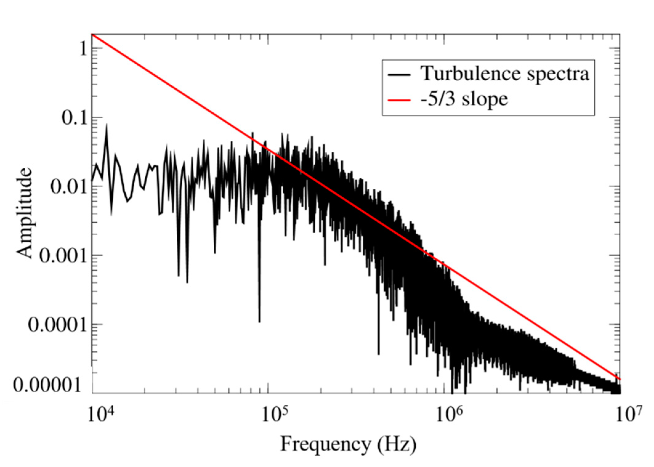
Figure 9.
Schematic of the configuration used to demonstrate design space exploration of vaporizing liquid jet in crossflow using GPML. Quantitative comparisons between the GPML predictions and truth models were made at four planes corresponding to x = 80, 120, 170, and 210 mm from the inlet.
Figure 9.
Schematic of the configuration used to demonstrate design space exploration of vaporizing liquid jet in crossflow using GPML. Quantitative comparisons between the GPML predictions and truth models were made at four planes corresponding to x = 80, 120, 170, and 210 mm from the inlet.

Figure 10.
Instantaneous spray field for three representative cases of momentum flux ratios of 5, 30, 120 showing qualitative differences in the spray field.
Figure 10.
Instantaneous spray field for three representative cases of momentum flux ratios of 5, 30, 120 showing qualitative differences in the spray field.

Figure 11.
Comparison between predictions from the GPML algorithm (referred to as predictions) with LES results (referred to as truth) for test points of q = 7 and 40. (a) Contours of velocity magnitude in the mid-plane of the flow domain; (b) variation of velocity magnitude along the y-axis at x = 80, 120, 170, and 210 mm.
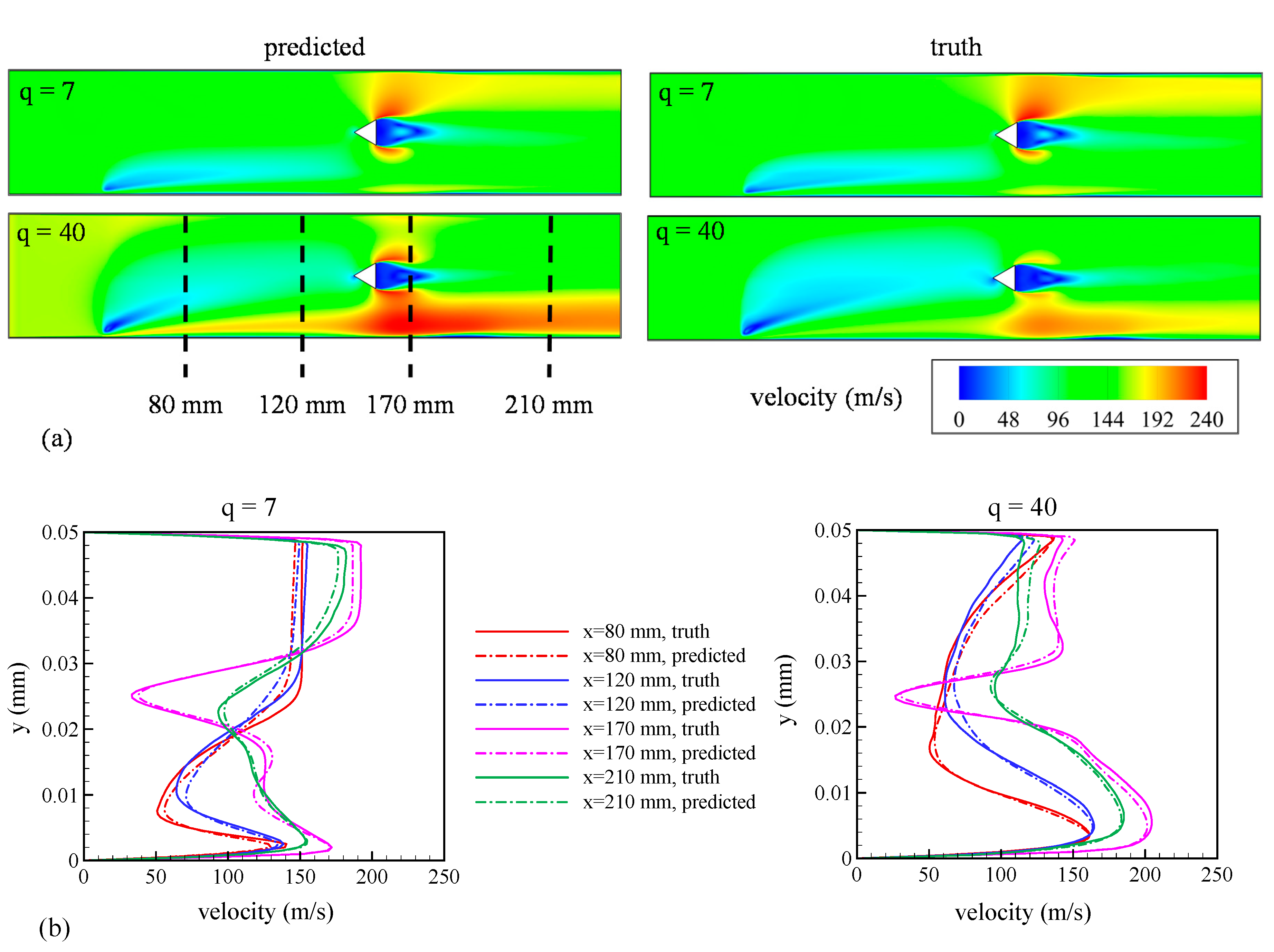
Figure 12.
Comparison between predictions from the GPML algorithm (referred to as predictions) with LES results (referred to as truth) for test points of q = 7 and 40. (a) Contours of TKE in the mid-plane of the flow domain; (b) variation of TKE along the y-axis at x = 80, 120, 170, and 210 mm.
Figure 12.
Comparison between predictions from the GPML algorithm (referred to as predictions) with LES results (referred to as truth) for test points of q = 7 and 40. (a) Contours of TKE in the mid-plane of the flow domain; (b) variation of TKE along the y-axis at x = 80, 120, 170, and 210 mm.

Figure 13.
Comparison between predictions from the GPML algorithm (referred to as predictions) with LES results (referred to as truth) for test points of q = 7 and 40. (a) Contours of pressure in the mid-plane of the flow domain; (b) variation of pressure along the y-axis at x = 80, 120, 170, and 210 mm.
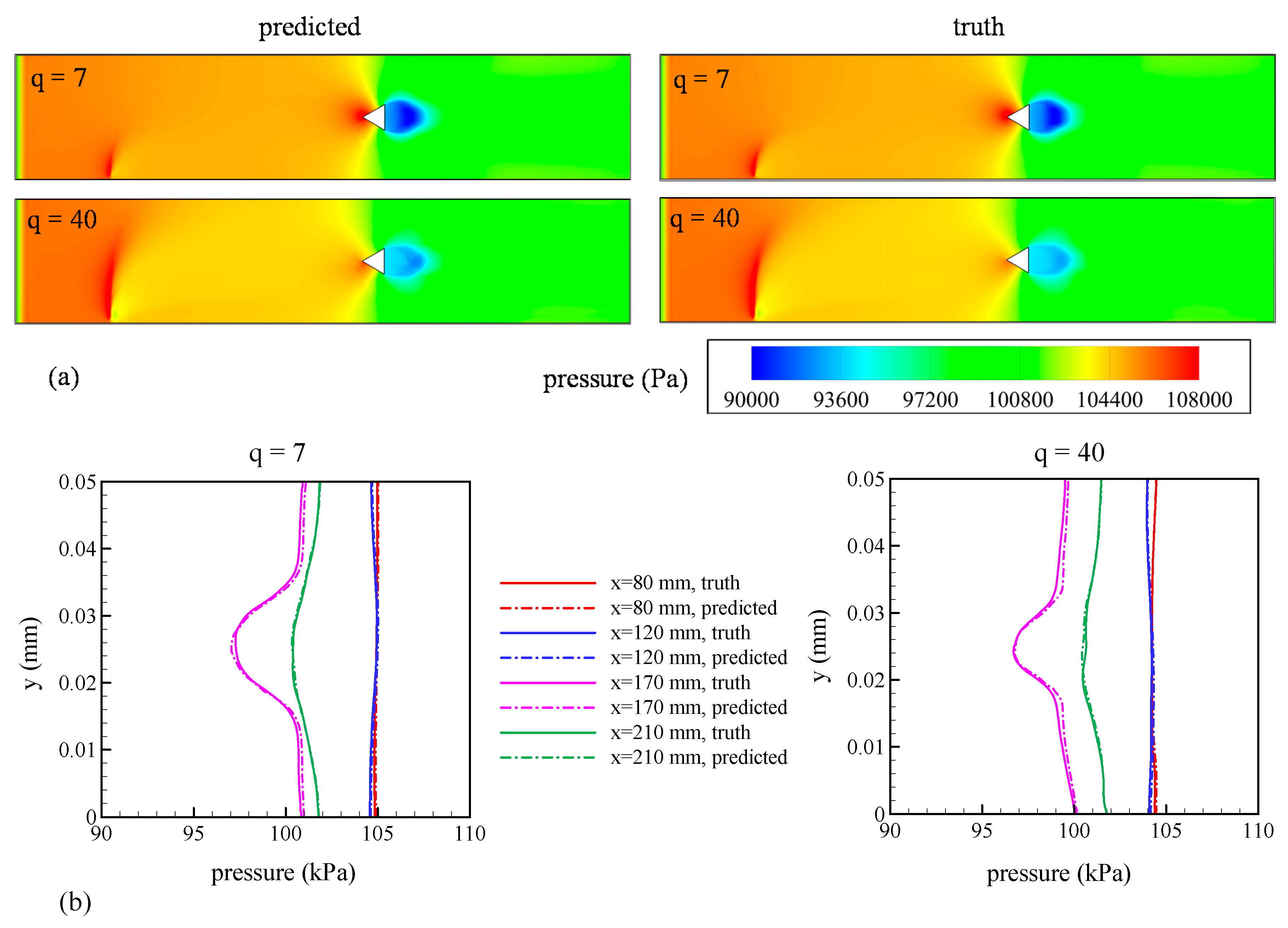
Figure 14.
Comparison between predictions from the GPML algorithm (referred to as predictions) with LES results (referred to as truth) for test points of q = 7 and 40. (a) Contours of temperature in the mid-plane of the flow domain; (b) variation of temperature along the y-axis at x = 80, 120, 170, and 210 mm.
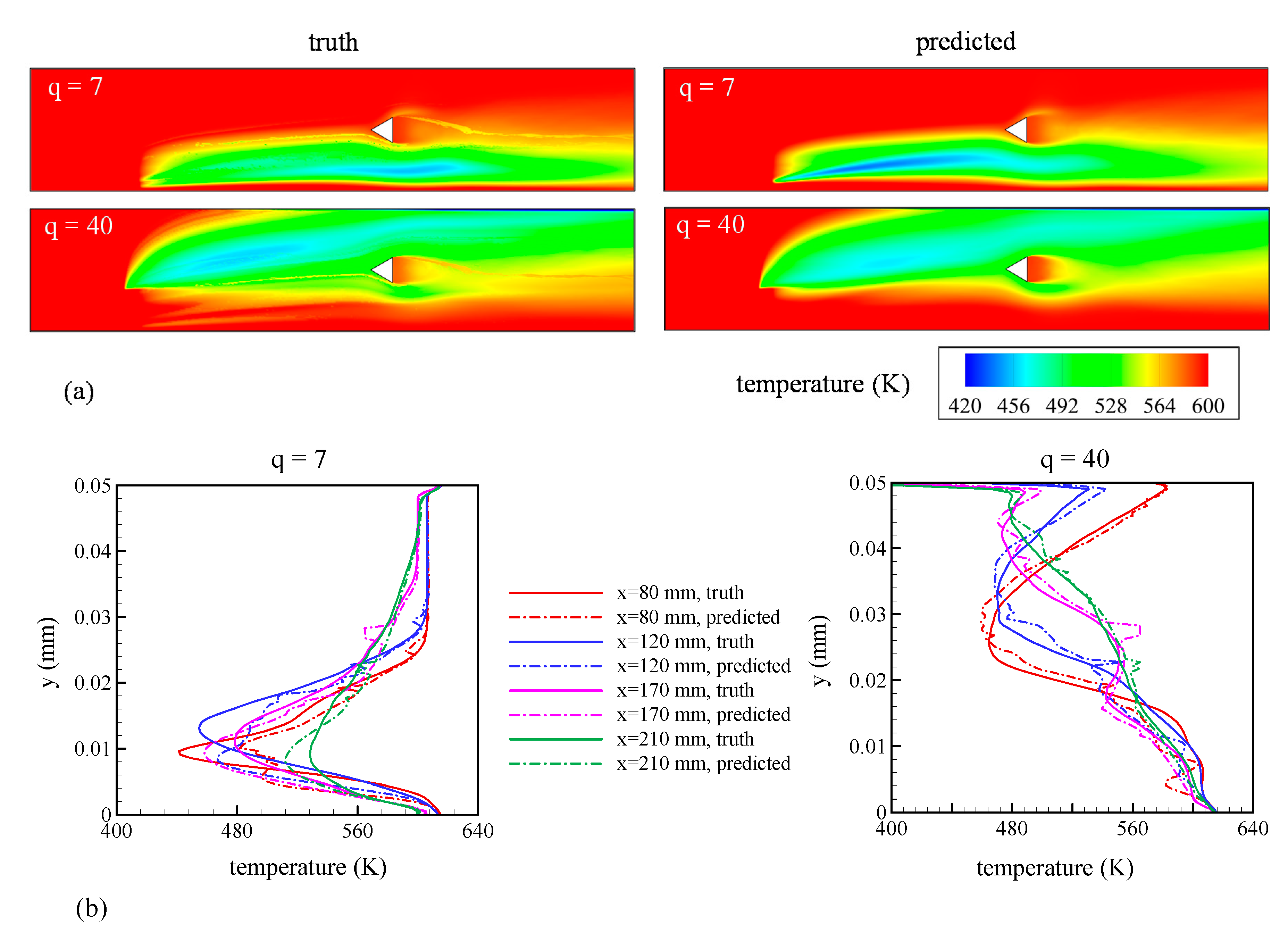
Figure 15.
Comparison between predictions from the GPML algorithm (referred to as predictions) with LES results (referred to as truth) for test points of q = 7 and 40. (a) Contours of liquid vapor fraction in the mid-plane of the flow domain; (b) variation of liquid vapor fraction along the y-axis at x = 80, 120, 170, and 210 mm.
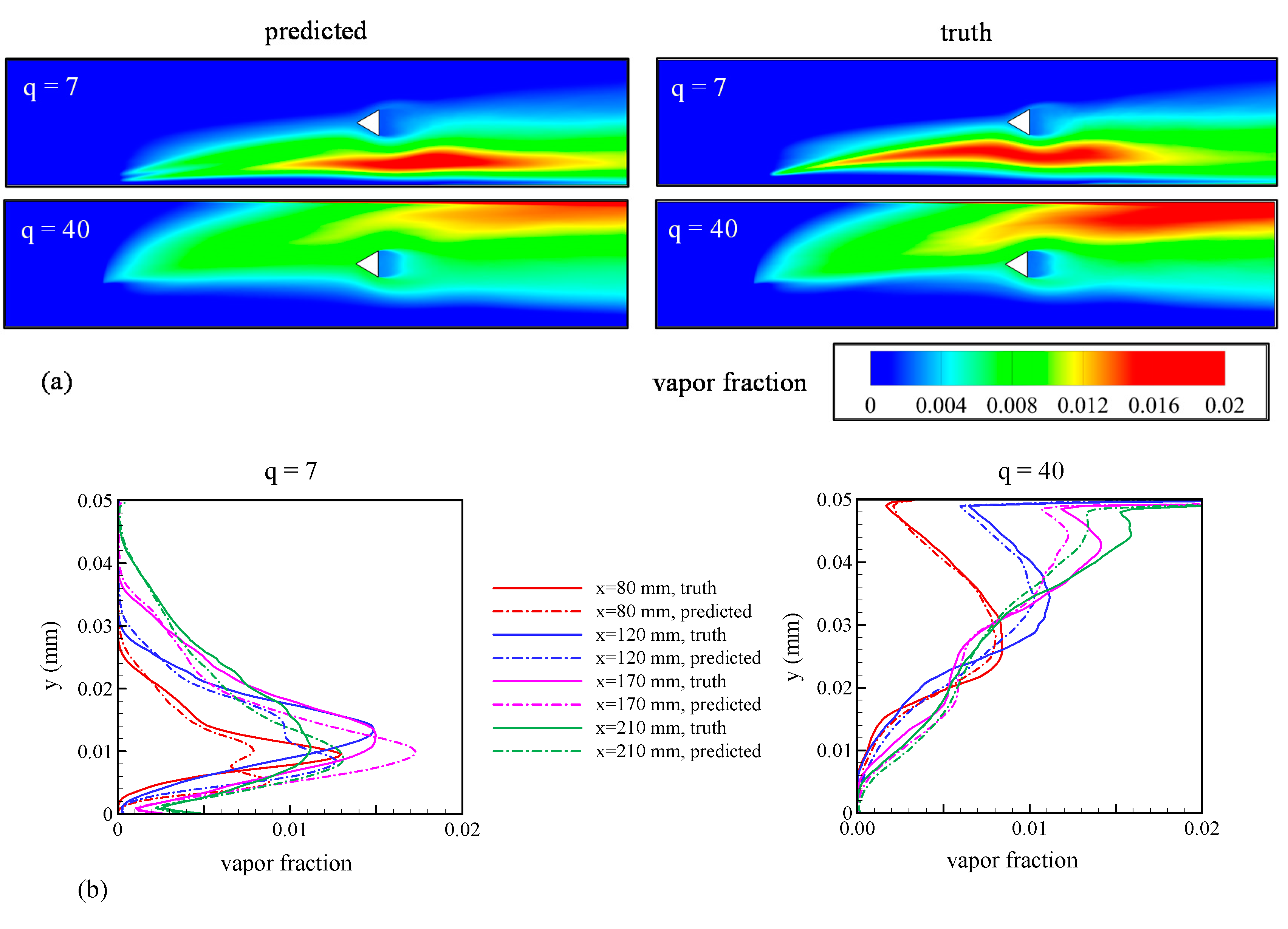
Figure 16.
Comparison between predictions from the GPML algorithm (referred to as predictions) with LES results (referred to as truth) for test points of q = 7 and 40. (a) SMD; (b) liquid jet penetration depth.
Figure 16.
Comparison between predictions from the GPML algorithm (referred to as predictions) with LES results (referred to as truth) for test points of q = 7 and 40. (a) SMD; (b) liquid jet penetration depth.

Table 1.
Operating conditions, physical properties, and relevant non-dimensional numbers used for model validation cases.
Table 1.
Operating conditions, physical properties, and relevant non-dimensional numbers used for model validation cases.
| Non-Vaporizing Case | Vaporization Case | |
|---|---|---|
| Ta (K) | 300 | 600 |
| Ua (m/s) | 116 | 166 |
| Uj (m/s) | 12.01 | 12.3 |
| ρa (kg/m3) | 1.18 | 0.62 |
| σo (N/m) | 7.28 × 10⁻² | 7.28 × 10⁻² |
| µa (Ns/m2) | 1.86 × 10⁻⁵ | 2.98 × 10⁻⁵ |
| q | 9 | 9 |
| We | 68 | 68 |
| Re | 2059.3 | 933.7 |
Table 2.
List of momentum flux ratio values for training the machine learning emulator.
| Training Dataset Identified by the Momentum Flux Ratio, q | ||||||
|---|---|---|---|---|---|---|
| 5 | 8 | 10 | 30 | 50 | 100 | 120 |
Table 3.
List of momentum flux ratio values to test the trained GPML algorithm.
| Testing Dataset Identified by the Momentum Flux Ratio, q | ||||||
|---|---|---|---|---|---|---|
| 7 | 9 | 20 | 40 | 65 | 90 | 110 |
© 2020 by the authors. Licensee MDPI, Basel, Switzerland. This article is an open access article distributed under the terms and conditions of the Creative Commons Attribution (CC BY) license (http://creativecommons.org/licenses/by/4.0/).
Share and Cite
MDPI and ACS Style
Ganti, H.; Kamin, M.; Khare, P. Design Space Exploration of Turbulent Multiphase Flows Using Machine Learning-Based Surrogate Model. Energies 2020, 13, 4565. https://doi.org/10.3390/en13174565
AMA Style
Ganti H, Kamin M, Khare P. Design Space Exploration of Turbulent Multiphase Flows Using Machine Learning-Based Surrogate Model. Energies. 2020; 13(17):4565. https://doi.org/10.3390/en13174565
Chicago/Turabian StyleGanti, Himakar, Manu Kamin, and Prashant Khare. 2020. "Design Space Exploration of Turbulent Multiphase Flows Using Machine Learning-Based Surrogate Model" Energies 13, no. 17: 4565. https://doi.org/10.3390/en13174565
Note that from the first issue of 2016, this journal uses article numbers instead of page numbers. See further details here.