Investigation of the Possibilities to Improve Hydrodynamic Performances of Micro-Hydrokinetic Turbines

Abstract
1. Introduction
2. Methods
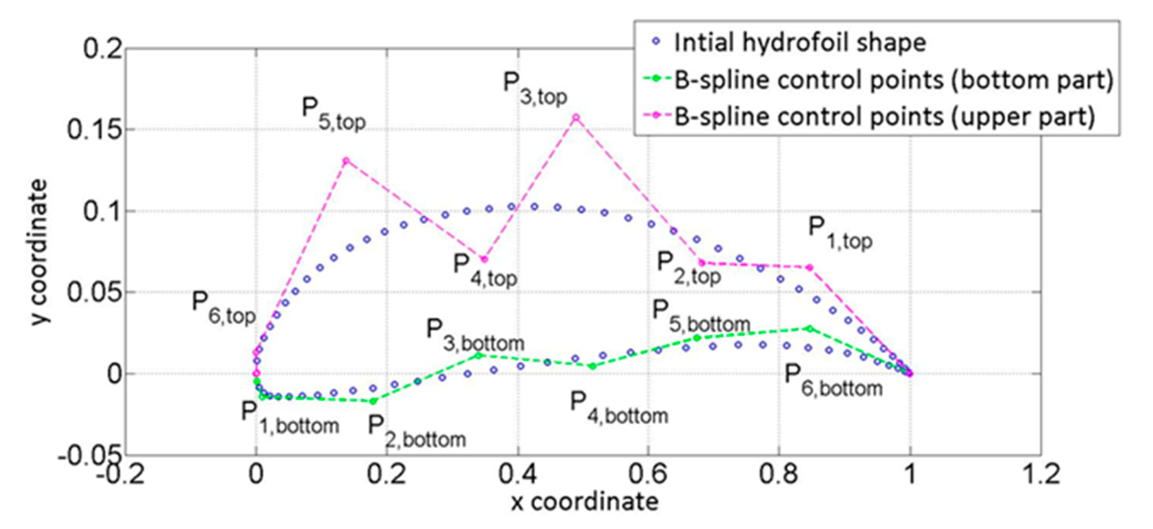
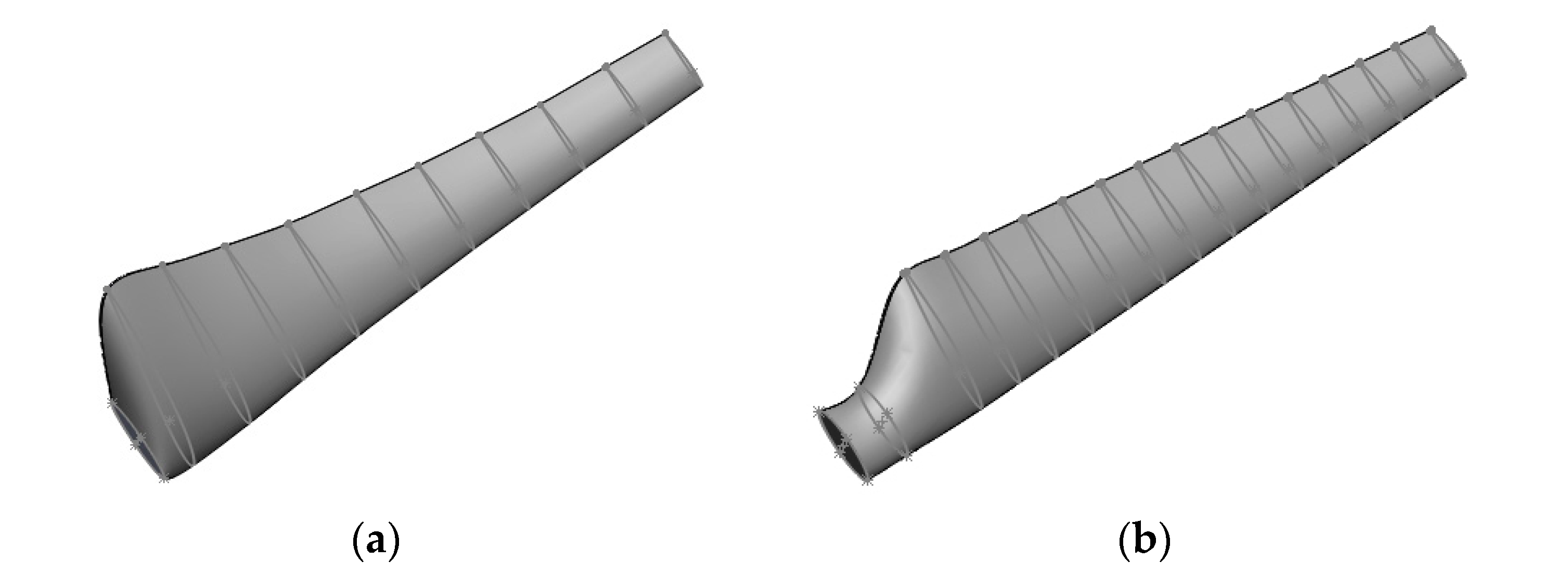
2.1. Rotor Design
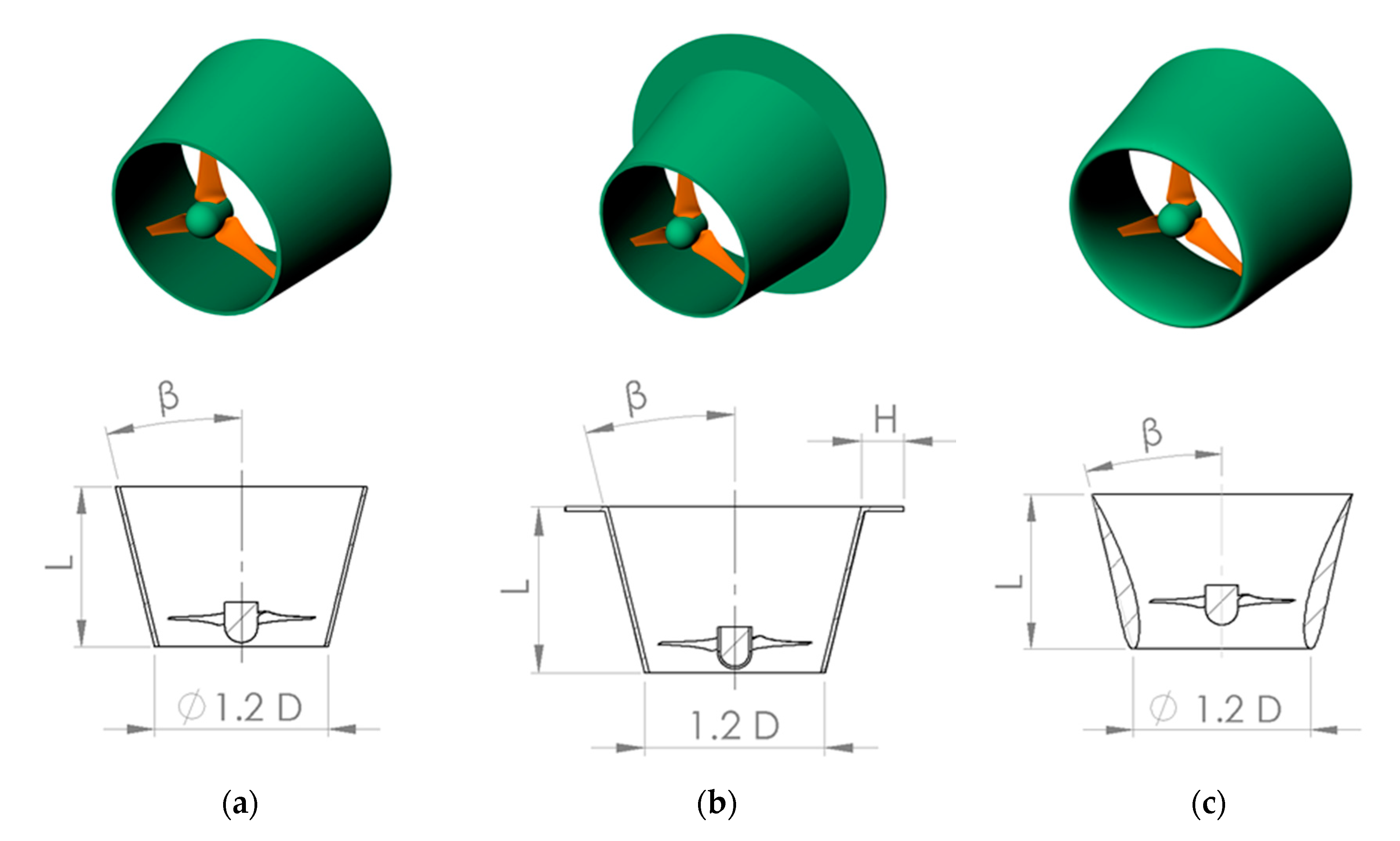
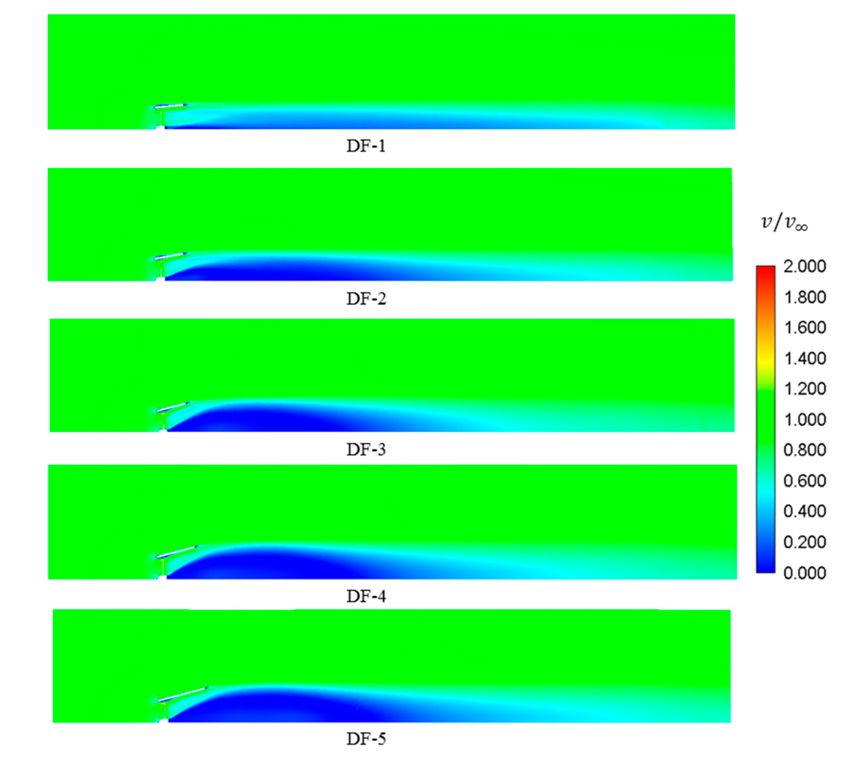
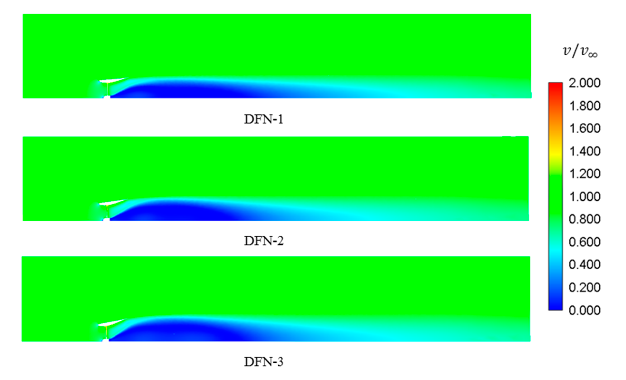
2.2. Diffuser Design
2.3. Numerical Methods
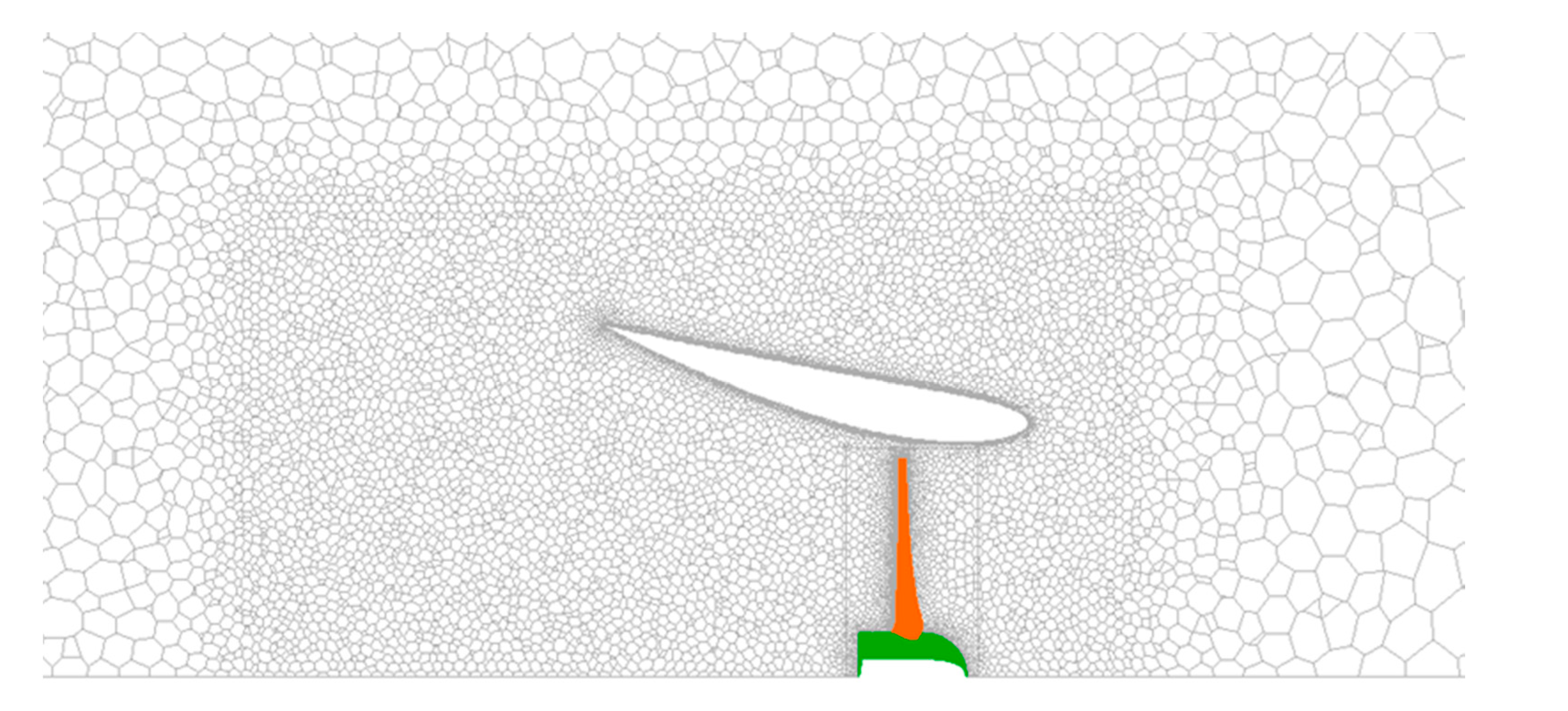
2.4. Computational Setup
2.5. Numerical Model Validation
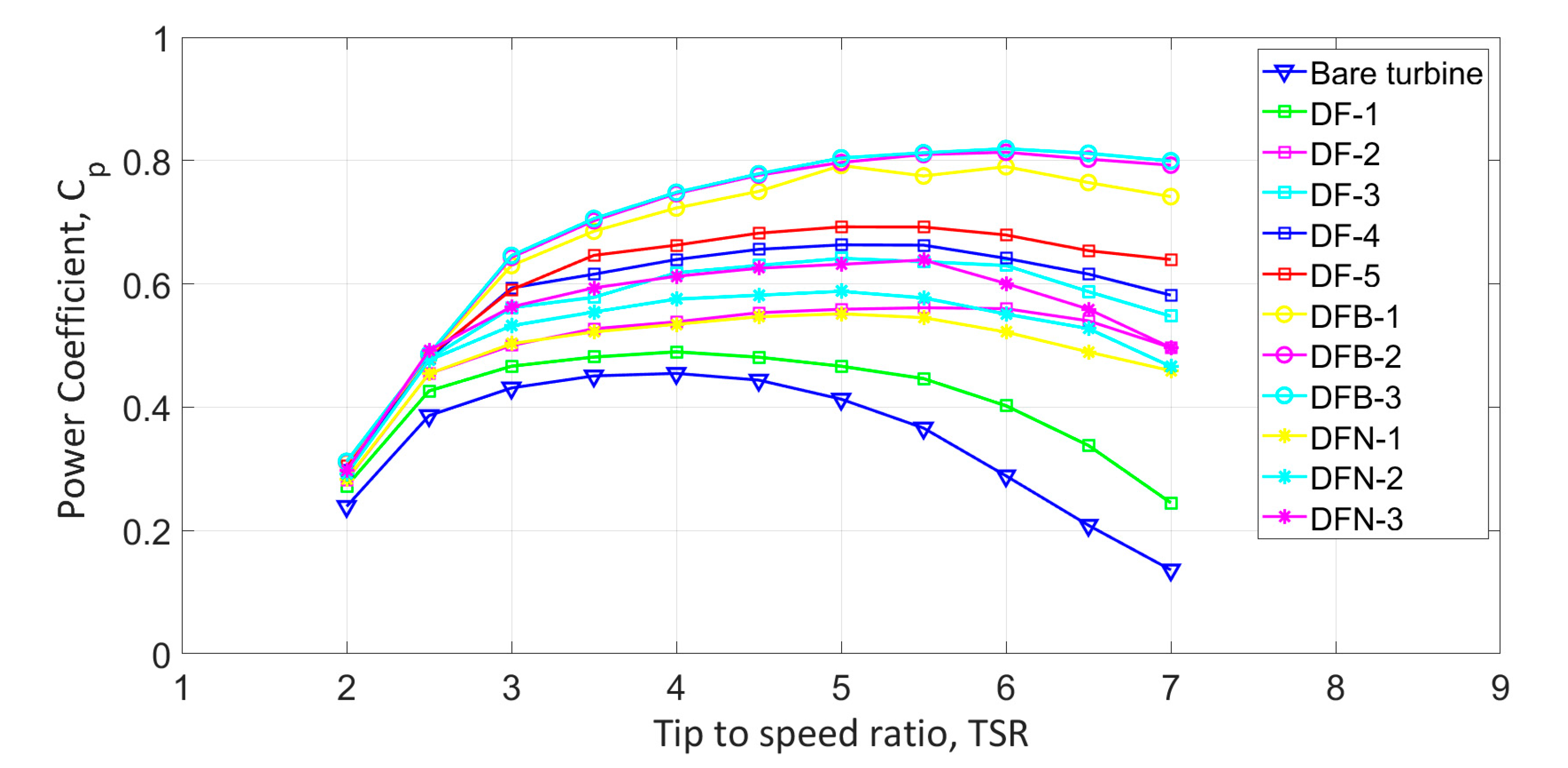
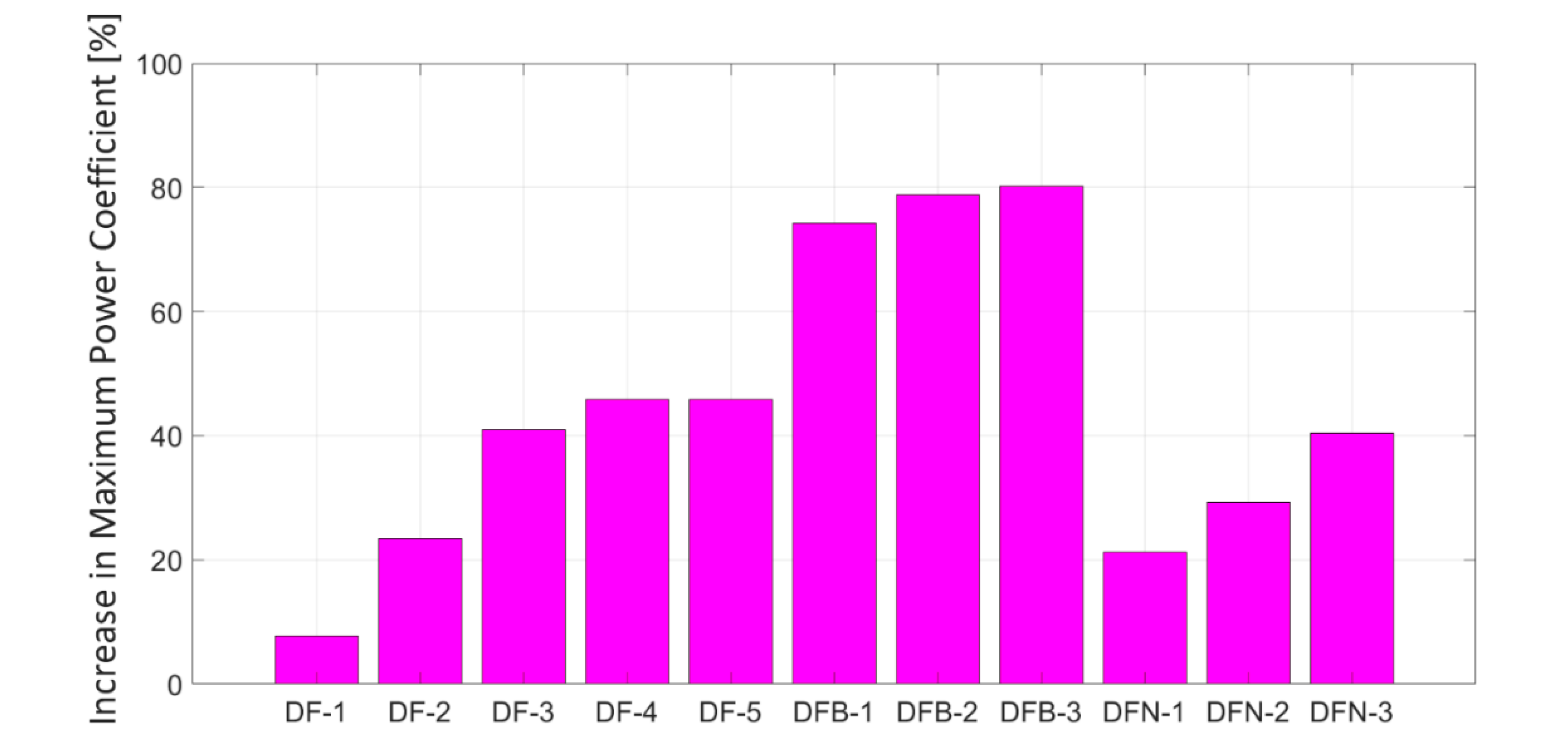
3. Results
4. Discussion
5. Conclusions
Author Contributions
Funding
Conflicts of Interest
Nomenclature
| Unit | Description | |
| - | axial induction factor | |
| - | angular induction factor | |
| B | - | blade number |
| - | drag coefficient | |
| - | lift coefficient | |
| - | power coefficient | |
| - | thrust coefficient | |
| D | m | diffuser diameter |
| m | blade chord length | |
| - | representative mesh size | |
| m/s | gravitational acceleration | |
| - | overall correction factor | |
| - | hub loss correction factor | |
| - | tip loss correction factor | |
| - | coefficient of pressure | |
| - | minimum coefficient of pressure | |
| m | diffuser length | |
| - | total number of mesh cells used for computation | |
| - | order of convergence | |
| Pa | atmospheric pressure | |
| Pa | vapor pressure | |
| W | effective power | |
| m | turbine radius | |
| - | grid refinement factor | |
| m | hub radius | |
| m/s | water velocity | |
| m/s | relative velocity | |
| - | weighting factors for lift coefficients | |
| - | weighting factors for drag coefficients | |
| - | weighting factors for minimum coefficients of pressure | |
| N | thrust force | |
| m3 | volume of the ith cell | |
| ° | angle of attack | |
| ° | design angle of attack | |
| ° | expansion or open angle of diffuser | |
| ° | blade pitch angle | |
| - | speed ratio at radius r | |
| ° | angle of relative flow | |
| kg/m3 | water density | |
| - | cavitation number | |
| rad/s | turbine rotational speed |
Acronyms
| BEM | Blade Element Momentum Theory |
| CAD | Computer-Aided Design |
| CFD | Computational Fluid Dynamics |
| CNC | Computer Numerical Control |
| GCI | Grid Convergence Index |
| MRF | Multiple Reference Frame |
| RANS | Reynolds-Averaged Navier-Stokes |
| TCP | Tidal Current Power |
| TSR | Tip to Speed Ratio |
References
- El-Zahaby, A.M.; Kabeel, A.E.; Elsayed, S.S.; Obiaa, M.F. CFD analysis of flow fields for shrouded wind turbine’s diffuser with different flange angles. Alex. Eng. J. 2017, 56, 171–179. [Google Scholar] [CrossRef]
- Wong, K.H.; Chong, W.T.; Yap, H.T.; Fazlizan, A.; Omar, W.Z.W.; Poh, S.C.; Hsiao, F.B. The design and flow simulation of a power-augmented shroud for urban wind turbine system. Energy Procedia 2014, 61, 1275–1278. [Google Scholar] [CrossRef]
- Abdelwaly, M.; El-Batsh, H.; Hanna, M.B. Numerical study for the flow field and power augmentation in a horizontal axis wind turbine. Sustain. Energy Technol. Assess. 2019, 31, 45–253. [Google Scholar] [CrossRef]
- Lipian, M.; Dobrev, I.; Karczewski, M.; Massouh, F.; Jozwik, K. Small wind turbine augmentation: Experimental investigations of shrouded- and twin-rotor wind turbine systems. Energy 2019, 186, 115855. [Google Scholar] [CrossRef]
- Siavash, N.K.; NajafI, G.; Hashjin, T.T.; Ghobadian, B.; Mahmoodi, E. Mathematical modeling of a horizontal axis shrouded wind turbine. Renew. Energy 2020, 146, 856–866. [Google Scholar] [CrossRef]
- Ghenai, C.; Salameh, T.; Janajreh, I. Modeling and Simulation of Shrouded Horizontal Axis Wind Turbine Using RANS Method. JJMIE 2017, 11, M235–M243. [Google Scholar]
- Siavash, N.K.; NajafI, G.; Hashjin, T.T.; Ghobadian, B.; Mahmoodi, E. An innovative variable shroud for micro wind turbines. Renew. Energy 2020, 145, 1061–1072. [Google Scholar] [CrossRef]
- Vaz, J.R.P.; Wood, D.H. Aerodynamic optimization of the blades of diffuser-augmented wind turbines. Energy Convers. Manag. 2016, 123, 35–45. [Google Scholar] [CrossRef]
- Barbosa, D.L.M.; Vaz, J.R.P.; Figueiredo, S.; Silva, M. An Investigation of a Mathematical Model for the Internal Velocity Profile of Conical Diffusers Applied to DAWTs. Ann. Acad. Bras. Ciênc. 2015, 87, 1133–1148. [Google Scholar] [CrossRef][Green Version]
- Hsiao, F.; Bai, F.; Wen-Tong, C. The Performance Test of Three Different Horizontal Axis Wind Turbine (HAWT) Blade Shapes Using Experimental and Numerical Methods. Energies 2013, 6, 2784–2803. [Google Scholar] [CrossRef]
- Wang, Q.Q.; Yin, R.; Yan, Y. Design and prediction hydrodynamic performance of horizontal axis micro-hydrokinetic river turbine. Renew. Energy 2019, 133, 91–102. [Google Scholar] [CrossRef]
- Batten, W.M.J.; Bahaj, A.S.; Molland, A.F.; Chaplin, J.R. The prediction of the hydrodynamic performance of marine current turbine. Renew. Energy 2008, 33, 1085–1096. [Google Scholar] [CrossRef]
- Liu, H.; Gu, Y.; Lin, Y.; Li, Y.; Li, W.; Zhou, H. Improved Blade Design for Tidal Current Turbines. Energies 2020, 13, 2642. [Google Scholar] [CrossRef]
- Song, M.; Kim, M.-C.; Do, I.-R.; Rhee, S.-H.; Lee, J.-H.; Hyun, B.-S. Numerical and experimental investigation on the performance of three newly designed 100 kW-class tidal current turbines. Int. J. Nav. Archit. Ocean Eng. 2012, 4, 241–255. [Google Scholar] [CrossRef]
- Chen, W.; Chen, H.; Lin, L.; Yu, Y. Tidal Current Power Resources and Influence of Sea-Level Rise in the Coastal Waters of Kinmen Island, Taiwan. Energies 2020, 10, 652. [Google Scholar] [CrossRef]
- Deng, G.; Zhang, Z.; Li, Y.; Liu, H.; Xu, W.; Pan, Y. Prospective of development of large-scale tidal current turbine array: An example numerical investigation of Zhejiang, China. Appl. Energy 2020, 264, 114621. [Google Scholar] [CrossRef]
- Sobczak, K.; Obidowski, D.; Reorowicz, P.; Marchewka, M. Numerical Investigations of the Savonius Turbine with Deformable Blades. Energies 2020, 13, 3717. [Google Scholar] [CrossRef]
- Rodrigues, S.P.; Brasil, A.P.; Jounior, A.C.P.; Salomon, L.B.R. Modeling of hydrokinetic turbine. In Proceedings of the 19th International Congress of Mechanical Engineering, Brasilia, Brazil, 5–9 November 2007. [Google Scholar]
- Knight, B.; Freda, R.; Young, Y.L.; Maki, K. Coupling Numerical Methods and Analytical Models for Ducted Turbines to Evaluate Designs. J. Mar. Sci. Eng. 2018, 6, 43. [Google Scholar] [CrossRef]
- Allsop, S.; Peyrard, C.; Thies, P.R.; Boulougouris, E.; Harrison, G.P. Hydrodynamic analysis of a ducted, open centre tidal stream turbine using blade element momentum theory. Ocean Eng. 2017, 141, 531–542. [Google Scholar] [CrossRef]
- Silva, P.A.S.F.; Rio Vaz, D.A.T.D.; Brittoa, V.; Oliveira, T.F.; Vaz, J.R.P.; Brasil Junior, A.C.P. A new approach for the design of diffuser-augmented hydro turbines using the blade element momentum. Energy Convers. Manag. 2018, 165, 801–814. [Google Scholar] [CrossRef]
- Shives, M.; Crawford, C. Developing an Empirical Model for Ducted Tidal Turbine Performance Using Numerical Simulation Results. Proc. Inst. Mech. Eng. Part A 2012, 226, 112–125. [Google Scholar] [CrossRef]
- Tampier, G.; Troncoso, C.; Zilic, F. Numerical analysis of a diffuser-augmented hydrokinetic turbine. Ocean Eng. 2017, 145, 138–147. [Google Scholar] [CrossRef]
- Wang, S.; Zhang, Y.; Xie, Y.; Xu, G.; Liu, K.; Zheng, Y. Hydrodynamic Analysis of Horizontal Axis Tidal Current Turbine under the Wave-Current Condition. J. Mar. Sci. Eng. 2020, 8, 562. [Google Scholar] [CrossRef]
- Song, K.; Wang, W.; Yan, Y. Numerical and experimental analysis of a diffuser-augmented micro-hydro turbine. Ocean Eng. 2019, 171, 580–602. [Google Scholar] [CrossRef]
- Rio Vaz, D.A.T.D.; Vaz, J.R.P.; Silva, A.S.F.P. An approach for the optimization of diffuser-augmented hydrokinetic blades free of cavitation. Energy Sustain. Dev. 2018, 45, 142–149. [Google Scholar] [CrossRef]
- Cresswell, N.W.; Ingrama, G.L.; Dominy, R.G. The impact of diffuser augmentation on a tidal stream turbine. Ocean Eng. 2015, 108, 155–163. [Google Scholar] [CrossRef]
- Gotelli, C.; Musa, M.; Guala, M.; Escauriaza, C. Experimental and Numerical Investigation of Wake Interactions of Marine Hydrokinetic Turbines. Energies 2019, 12, 3188. [Google Scholar] [CrossRef]
- Bai, G.; Li, J.; Fan, P.; Li, G. Numerical investigations of the effects of different arrays on power extractions of horizontal axis tidal current turbines. Renew. Energy 2013, 53, 180–186. [Google Scholar] [CrossRef]
- Belloni, C.S.K.; Willden, R.H.J.; Houlsby, G.T. An investigation of ducted and open-centre tidal turbines employing CFD-embedded BEM. Renew. Energy 2017, 108, 622–634. [Google Scholar] [CrossRef]
- Góralczyk, A.; Adamkowski, A. Model of a ducted axial-flow hydrokinetic turbine—Results of experimental and numerical examination. Pol. Marit. Res. 2018, 25, 113–122. [Google Scholar] [CrossRef]
- Tian, W.; Mao, Z.; Ding, H. Design, test and numerical simulation of low-speed horizontal axis hydrokinetic turbine. Int. J. Nav. Archit. Ocean Eng. 2018, 10, 782–793. [Google Scholar] [CrossRef]
- Riglin, J.; Schleicher, W.C.; Oztekin, A. Numerical analysis of shrouded a micro-kinetic turbine unit. J. Hydraul. Res. 2015, 53, 526–531. [Google Scholar] [CrossRef]
- Li, Z.; Zheng, X. Review of design optimization methods for turbomachinery aerodynamics. Prog. Aerosp. Sci. 2017, 93, 1–23. [Google Scholar] [CrossRef]
- Manwell, J.F.; Mc, J.G.; Rogers, A.L. Wind energy explained: Theory Design and Application; John Wiley & Sons Ltd.: Chichester, UK, 2002. [Google Scholar]
- Goundar, J.N.M.; Rafiuddin Ahmed, M. Design of horizontal axis tidal current turbine. Appl. Energy 2013, 111, 161–174. [Google Scholar] [CrossRef]
- Drela, M.; Youngren, H. Xfoil, Subsonic Airfoil Development System. Available online: http://web.mit.edu/drela/Public/web/xfoil/ (accessed on 13 June 2020).
- Selvan, K.M. On the effect of shape parametrization on airfoil shape optimization. Int. J. Res. Eng. Technol. 2015, 4, 123–133. [Google Scholar]
- Barbarić, M.; Guzović, Z. Design of hydrofoils for small-scaled hydrokinetic turbines using population-based algorithm. In Proceedings of the 12th Conference on Sustainable Development of Energy, Water and Environment Systems—SDEWES 2017, Dubrovnik, Croatia, 4–8 October 2017. [Google Scholar]
- Lain, S.; Contreras, L.T.; Lopez, O. A review on computational fluid dynamics modelling and simulation of horizontal axis hydrokinetic turbines. J. Braz. Soc. Mech. Sci. 2019, 41, 375. [Google Scholar] [CrossRef]
- Alfonsi, G. Reynolds-Averaged Navier-Stokes Equations for Turbulence Modelling. Appl. Mech. Rev. 2009, 62, 040802. [Google Scholar] [CrossRef]
- ANSYS. ANSYS Fluent Theory Guide; ANSYS Inc.: Canonsburg, PA, USA, 2017. [Google Scholar]
- Celik, I.B. Procedure for estimation and reporting of uncertainty due to discretization in CFD applications. J. Fluids Eng. Trans. ASME 2008, 130, 078001. [Google Scholar]
- Sosnowski, M.; Gnatowska, R.; Grabowska, K.; Krzywanski, J.; Jamrozik, A. Numerical Analysis of Flow in Building Arrangement: Computational Domain Discretization. Appl. Sci. 2019, 9, 941. [Google Scholar] [CrossRef]
- Noruzi, R.; Vahidzadeh, M.; Riasi, A. Design, analysis and predicting hydrokinetic performance of a horizontal marine current axial turbine by consideration of turbine installation depth. Ocean Eng. 2015, 108, 789–798. [Google Scholar] [CrossRef]
- Kwaśniewski, L. Application of grid convergence index in FE computation. Bull. Pol. Acad. Sci. Tech. Sci. 2013, 61, 123–128. [Google Scholar] [CrossRef]


| Type | L (m) | β (°) | H/D |
|---|---|---|---|
| DF-1 | 0.75D | 5 | - |
| DF-2 | 0.75D | 10 | - |
| DF-3 | 0.75D | 15 | - |
| DF-4 | 1D | 15 | - |
| DF-5 | 1.25D | 15 | - |
| DFB-1 | 0.75D | 15 | 0.25 |
| DFB-2 | 1D | 15 | 0.25 |
| DFB-3 | 1.25D | 15 | 0.25 |
| DFN-1 | 1D | 7 | - |
| DFN-2 | 1D | 10 | - |
| DFN-3 | 1D | 13 | - |
| Mesh | N | ϕ | rij | ε | p | |||
|---|---|---|---|---|---|---|---|---|
| 1 | 2.5 Million | 0.8024 | 1.56 | −0.034 | 0.2764 monotonic convergence | 1.48 | 0.4% | 0.63% |
| 2 | 1.6 Million | 0.8147 | 2.03 | −0.0123 | ||||
| 3 | 0.8 Million | 0.8181 | - | - |
© 2020 by the authors. Licensee MDPI, Basel, Switzerland. This article is an open access article distributed under the terms and conditions of the Creative Commons Attribution (CC BY) license (http://creativecommons.org/licenses/by/4.0/).
Share and Cite
Barbarić, M.; Guzović, Z. Investigation of the Possibilities to Improve Hydrodynamic Performances of Micro-Hydrokinetic Turbines. Energies 2020, 13, 4560. https://doi.org/10.3390/en13174560
Barbarić M, Guzović Z. Investigation of the Possibilities to Improve Hydrodynamic Performances of Micro-Hydrokinetic Turbines. Energies. 2020; 13(17):4560. https://doi.org/10.3390/en13174560
Chicago/Turabian StyleBarbarić, Marina, and Zvonimir Guzović. 2020. "Investigation of the Possibilities to Improve Hydrodynamic Performances of Micro-Hydrokinetic Turbines" Energies 13, no. 17: 4560. https://doi.org/10.3390/en13174560
APA StyleBarbarić, M., & Guzović, Z. (2020). Investigation of the Possibilities to Improve Hydrodynamic Performances of Micro-Hydrokinetic Turbines. Energies, 13(17), 4560. https://doi.org/10.3390/en13174560