Electro-Hydraulic Transient Regimes in Isolated Pumps Working as Turbines with Self-Excited Induction Generators

Abstract

The use of pumps working as turbines (PATs) is a sustainable technical measure that contributes to the improvement of energy efficiency in water systems. However, its performance analysis in off-grid recovery systems is a complex task that must consider both hydraulic (PAT) and electrical machines (typically a self-excited induction generator-SEIG). Aside from several kinds of research that analyze the PAT-SEIG behavior under steady-state constant hydraulic and electrical conditions, this research focuses on the analysis of PAT-SEIG transient regimes, by analyzing their variation when a sudden change occurs in the hydraulic or electrical components. Analytical models were developed to represent the operation of SEIG, PAT, and the PAT-SEIG coupled system. Hydraulic and electromechanical experimental tests validated these models. An excellent fit was obtained when analytical and experimental values were compared. With these models, the impact on the operation of the PAT-SEIG system was examined when sudden change occurred in the excitation capacitances, resistive loads, or recovered head. With a sudden increase of resistive load, the hydraulic power and SEIG stator current remain almost constant. However, there is an increase of SEIG reactive power, decreasing the PAT-SEIG efficiency. Also, with a sudden increase of SEIG capacitors or PAT hydraulic head, the SEIG stator current increases once and not again, while PAT-SEIG efficiency decreases, but the induction generator can be overloaded. The development of this research is key to the advancement of future models which can analyze the coupling of micro-hydropower solutions.

1. Introduction

Micro-hydro power generation has a high potential to be used in many water sector applications where there is an excess of energy [1]. The sustainability improvement is focused on taking advantage of the hydraulic energy of water systems (i.e., pressurized or free surface) and transforming it into electric energy. This transformation needs the two main elements: a turbine and an electric generator. Both elements operate together, and therefore the analysis of the recovery system must be developed jointly for the water managers to maximize the efficiency improvement in their water systems [2]. One challenge regarding micro-hydro turbines is the cost of the turbine, which increases the initial investment, making it almost impracticable in small communities or off-grid locations [3]. One solution is the use of pumps working as turbines (PATs) since they can work in reversed mode, in a similar way as a turbine [4]. PAT is a hydraulic machine, and it requires an electrical machine to operate. Typically, commercial pumps use induction machines to convert electric power into mechanical power, and this machine is one of the most cost-effective available solutions in the market. Induction machines can also work in generator mode, connected to the grid or off-grid.

In this work, the use of PAT in rural areas where grid connection may not be possible due to physical or legal constraints will be analyzed. To work in off-grid mode, the induction generator requires an external source of reactive power. The reactive power source can be a battery coupled to the machine by an inverter or a set of capacitors connected directly to the machine. The latter solution is called a self-excited induction generator (SEIG). PAT and SEIG are coupled mechanically by a shaft operating as PAT+SEIG system (Figure 1). The analysis of this symbiosis is crucial since the global efficiency of the recovery system (PAT+SEIG) depends on each one of their efficiencies (i.e., fluid mechanical and electrical). When these efficiencies are analyzed, the maximum efficiency is located on different points. Therefore, the maximum efficiency in the PAT cannot be coincident with the maximum efficiency of the SEIG [5]. Another important aspect of these hydraulic-electromechanical systems is the investigation of transient behaviors due to sudden changes. The study of these types of influences in the system is of the utmost importance due to their effects on control stability. For example, in [6], a state feedback predictive control was applied to a hydro-turbine governing system to increase the control performance in the case of external disturbances. Also, the effect of a sudden drop in the prime mover speed of a SEIG (without the PAT) was analyzed in [7]. These effects, of sudden changes, may have an additional influence in PAT-SEIG systems during off-grid operation.

The modeling of water systems, as well as the PATs regulation, were considered in many research publications. Carravetta et al. [8] defined the different regulation types (i.e., hydraulic, electrical, and hydraulic-electrical modes). These regulation modes were compared in different water systems showing the variability of energy recovery according to the chosen strategy [9]. Different research works also focused on PAT operation and efficiency. The analysis of the tip clearance on pressure fluctuation intensity in PATs [10], cavitation performance and forces [11], or analysis of leakages [12], are also important factors to be considered. All these analyses are crucial to improve the management of the PATs. Accordingly, different optimization strategies were considered to locate the recovery systems in water systems. [13] summarized the different optimization procedures to maximize the recovered energy in the water sector. Other researches also considered the maximization of recovered energy in water systems [14], but few considered the singularity for PATs operating in off-grid mode. In this operation mode, the electrical efficiency acquires a greater significance, and the maximization of the recovered energy requires a detailed analysis due to the associated complexity.

Hence, this research focuses on analyzing the binomial hydraulic-electromechanical interaction system of Figure 1. It is composed of a pump working as a turbine (PAT) and an induction machine working as a self-excited induction generator (SEIG), which is connected to the PAT via a mechanical shaft. Inputs for the PAT+SEIG system are a differential pressure for the PAT imposed by upstream-downstream tanks, the electrical load, and the excitation capacitor bank of the SEIG. A hydraulic-electromechanical model was developed to simulate the behavior of the PAT and SEIG systems. The developed model was tuned with experimental data. The final model was validated, and it showed sufficiently accurate results for the overall system dynamics.

These analyses are representative of the system, and they allow operators to know the interaction between water and electrical machine through their different components of each part. This analysis is an important step forward to analyze the behavior of PAT+SEIG systems, which could be associated in serial or parallel in water pipe systems.

2. Self-Excited Induction Generator Model

The self-excited induction generator (SEIG) was modeled using a dq0 transformation [15] to capture the transient behavior of its electrical and magnetic quantities. Also, the change of the machine’s magnetizing inductance, $L_M$, due to its non-linear B(H) characteristic was considered, as it highly influences the choice of the correct capacitance to self-excite the machine for a specific operating point [5] (different speeds and loads). The evolution of the magnetizing inductance as a function of the magnetization flux used here was determined experimentally in [5], for the induction machine used in the experimental results. The SEIG model was developed in Simulink, and it can be observed in Figure 2.

The dq induction machine model was developed using a stationary reference frame, aligned with phase A of the stator windings. Being all machine phases symmetric, the homopolar term will be null. The dq stator and rotor equations are shown in (1) to (4). In (1) and (2) $u_{d_s}$, $u_{q_s}$, $i_{d_s}$ and $i_{q_s}$ are the d and q axes stator voltages and currents, respectively, being its units V and A. ${\Psi }_{d_s}$ and ${\Psi }_{q_s}$ are the d and q axes stator linkage fluxes and $R_s$ is the stator phase resistance. In (3) and (4), $i_{d_r}$, $i_{q_r}$, ${\Psi }_{d_r}$ and ${\Psi }_{q_r}$ are the d and q axes rotor currents and linkage fluxes, respectively, $R_r$ is the rotor phase resistance (referred to the stator), and ${\omega }_r$ is the rotor angular speed in rad/s [15].

$$u_{d_s}=R_s{i}_{d_s}+\frac{d{\Psi }_{d_s}}{dt}$$

(1)

$$u_{q_s}=R_s{i}_{q_s}+\frac{d{\Psi }_{q_s}}{dt}$$

(2)

$$0=R_r{i}_{d_r}+\frac{d{\Psi }_{d_r}}{dt}-{\omega }_r{\Psi }_{q_r}$$

(3)

$$0=R_r{i}_{q_r}+\frac{d{\Psi }_{q_r}}{dt}+{\omega }_r{\Psi }_{d_r}$$

(4)

The relation between the stator and rotor linkage fluxes and the corresponding currents are presented in (5)–(8).

$${\Psi }_{d_s}=L_s{i}_{d_s}+L_M{i}_{d_r}$$

(5)

$${\Psi }_{q_s}=L_s{i}_{q_s}+L_M{i}_{q_r}$$

(6)

$${\Psi }_{d_r}=L_r{i}_{d_r}+L_M{i}_{d_s}$$

(7)

$${\Psi }_{q_r}=L_r{i}_{q_r}+L_M{i}_{q_s}$$

(8)

The electromagnetic torque, $T_{em},$ developed by the induction machine can be computed by (9), where $n_{pp}$ is the pair poles.

$$T_{em}=\frac{3}{2}{n}_{pp}\left({\Psi }_{d_s}{i}_{q_s}-{\Psi }_{q_s}{i}_{d_s}\right)$$

(9)

After the computation of the torque, the machine’s stator voltage and currents are converted into the three-phase quantities, a, b, and c, so that they can be compared with experimental values.

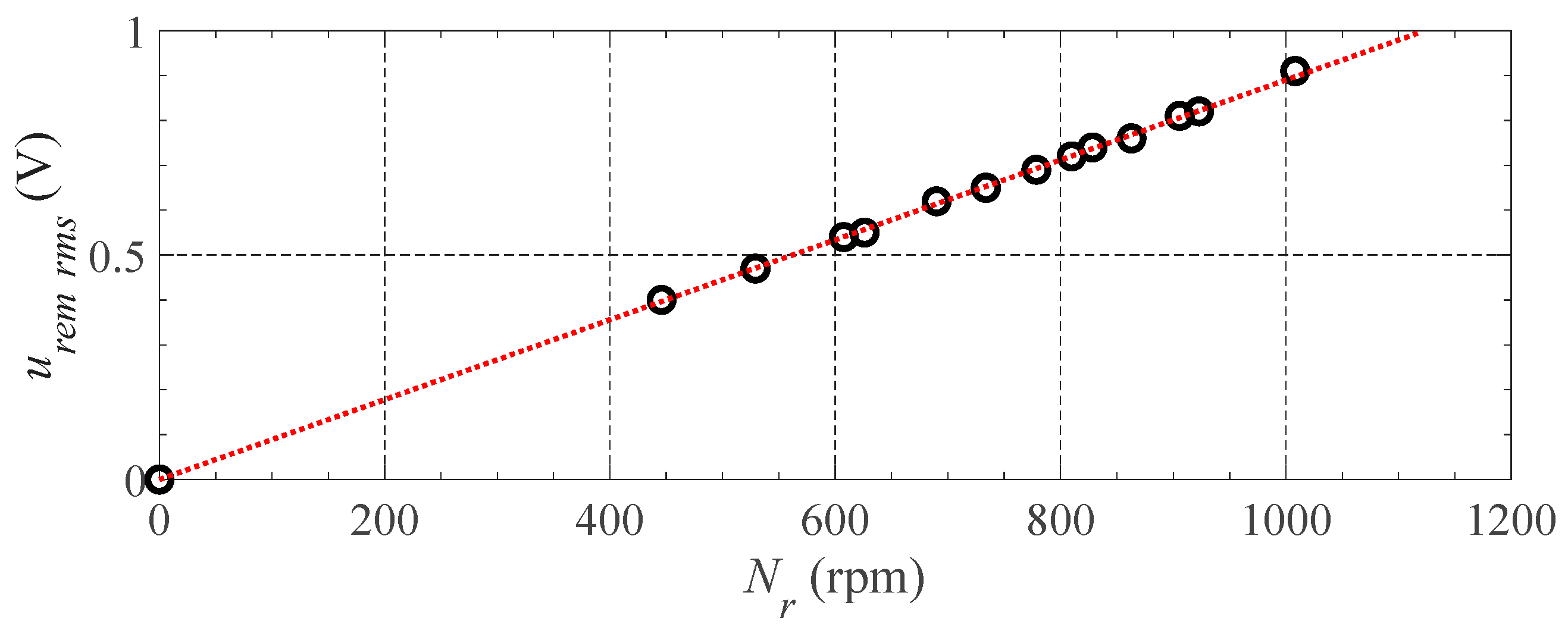
2.1. Magnetizing Inductance

As shown in [5], the SEIG model accuracy drastically increases when considering the variation of the magnetizing inductance, $L_M$, with the magnitude of the magnetization flux, ${\varphi }_M$. More specifically, for different resistive loads (R_L = 120, 200 and 600 Ω), the deviation between experimental and numerical induction generator model decreased by about 37%, to an average deviation of 10.7%. The evolution of $L_M$ with the magnetization flux was obtained experimentally in [5] and was approximated by the polynomial Equation in (10). This equation shows the experimentally calculated magnetizing inductance as a function of ${\varphi }_m$ for the range of frequencies 20–60 Hz.

The effect of the magnetic flux in $L_M$ was included in the dq SEIG model through Equations (5)–(8). In each time instant, the model calculates the magnetic flux of the SEIG and chooses the correct value of $L_M$. As the magnetic flux depends on the stator and rotor’s currents, the calculation of $L_M$ must be an iterative process in each time step. Fernandes et al. [5] defined the magnetizing inductance by the following equation:

$$L_M\left({\varphi }_M\right)=0.2192{\left({\varphi }_M\right)}^3-0.8093{\left({\varphi }_M\right)}^2+0.5531{\varphi }_M+0.53$$

(10)

The magnetization flux can be computed using (11), where ${\varphi }_{d_m}$ and ${\varphi }_{q_m}$ are the d and q axes magnetization fluxes, which can be obtained using (12) and (13).

$${\varphi }_m=\sqrt{{\varphi }_d{{}_m}^2+{\varphi }_q{{}_m}^2}$$

(11)

$${\varphi }_d{}_m={\Psi }_{d_s}-L_s{i}_{d_s}$$

(12)

$${\varphi }_q{}_m={\Psi }_{q_s}-L_s{i}_{q_s}$$

(13)

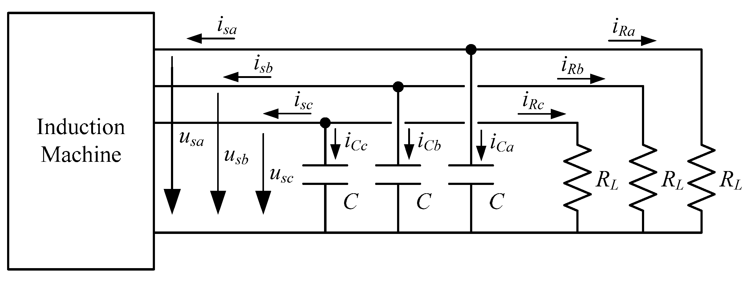
2.2. Capacitor and Electrical Load Models

The SEIG required a set of capacitors (i.e., one per phase) to self-excite. The capacitors are responsible for providing the required reactive power for the induction machine to create the rotating magnetic field. However, to start the self-excitation process, the capacitors require a voltage to provide reactive power. This means that, with the induction machine rotating, no machine voltage is induced until provided with reactive power, and no reactive power is produced without applying a voltage to the capacitors. Therefore, to start the excitation process, it is required an initial voltage. This initial voltage can be stored in the capacitors, with an initial charge, or provided by the remnant voltage induced at the induction machine’s stator terminals due to asymmetries in its magnetic circuit. The residue voltage induced by the induction generator in our system was enough to start the self-excitation process. This remnant induced voltage was measured experimentally for different speeds (Figure 3). This shows the phase-to-neutral rms value of the remnant induced voltage as a function of its angular speed, $N_r$. Each phase remnant voltage can be calculated from (14).

$$u_{{rem}_{rms}}=0.00086N_r (R^2=0.999)$$

(14)

Figure 4 shows the capacitor and load with the induction machine in parallel. The set of equations that expresses its behavior is given by (15). The capacitor bank receives the stator current of the induction machine and the current of the resistive load. It calculates the stator voltage, which is required for the induction machine and resistive blocks. In (15), $u_{s_{a,b,c}}$ and $i_{s_{a,b,c}}$ are the stator voltage and current of each machine’s phase, $i_{R_{a,b,c}}$ are the load current of each load phase, and $u_{{rem}_{a,b,c}}$ are the induced remnant voltages in (14).

$$\begin{array}{cc}{u}_{s_{a,b,c}}=u_{C_{a,b,c}}& =\frac{1}{C}\int i_{C_{a,b,c}}dt+u_{{rem}_{a,b,c}}\hfill \\ & =\frac{1}{C}\int -\left(i_{s_{a,b,c}} + i_{R_{a,b,c}}\right)dt+u_{{rem}_{a,b,c}}\hfill \\ & =-\frac{1}{C}\int \left(i_{s_{a,b,c}}+\frac{U_{s_{a,b,c}}}{R}\right)dt+u_{{rem}_{a,b,c}}\end{array}$$

(15)

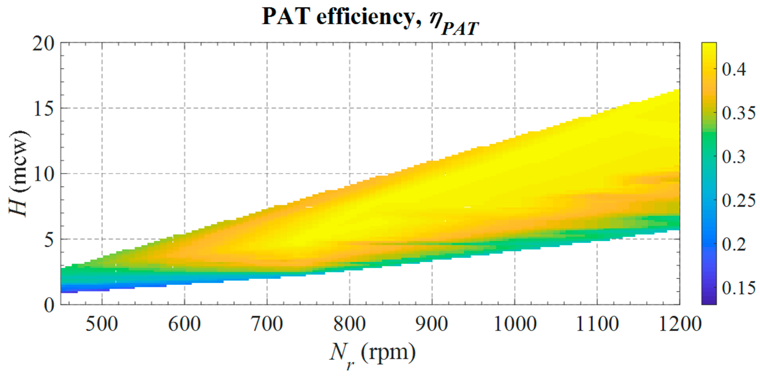
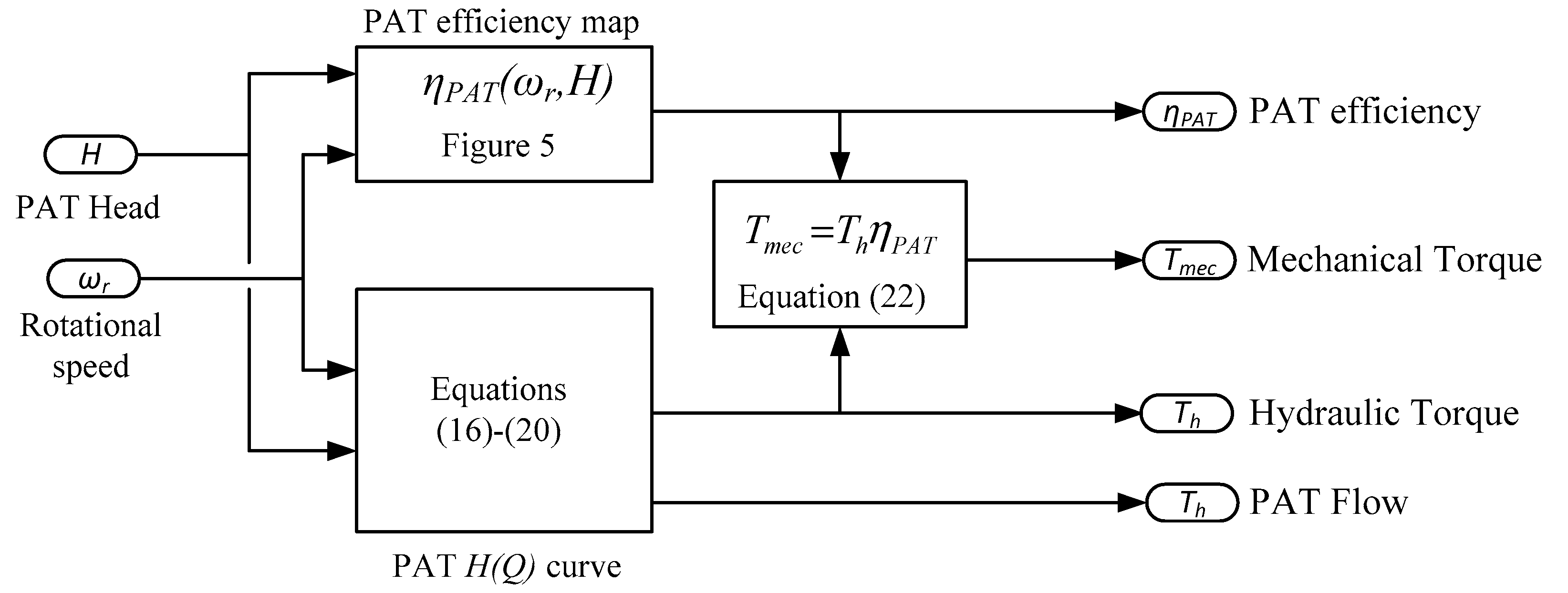
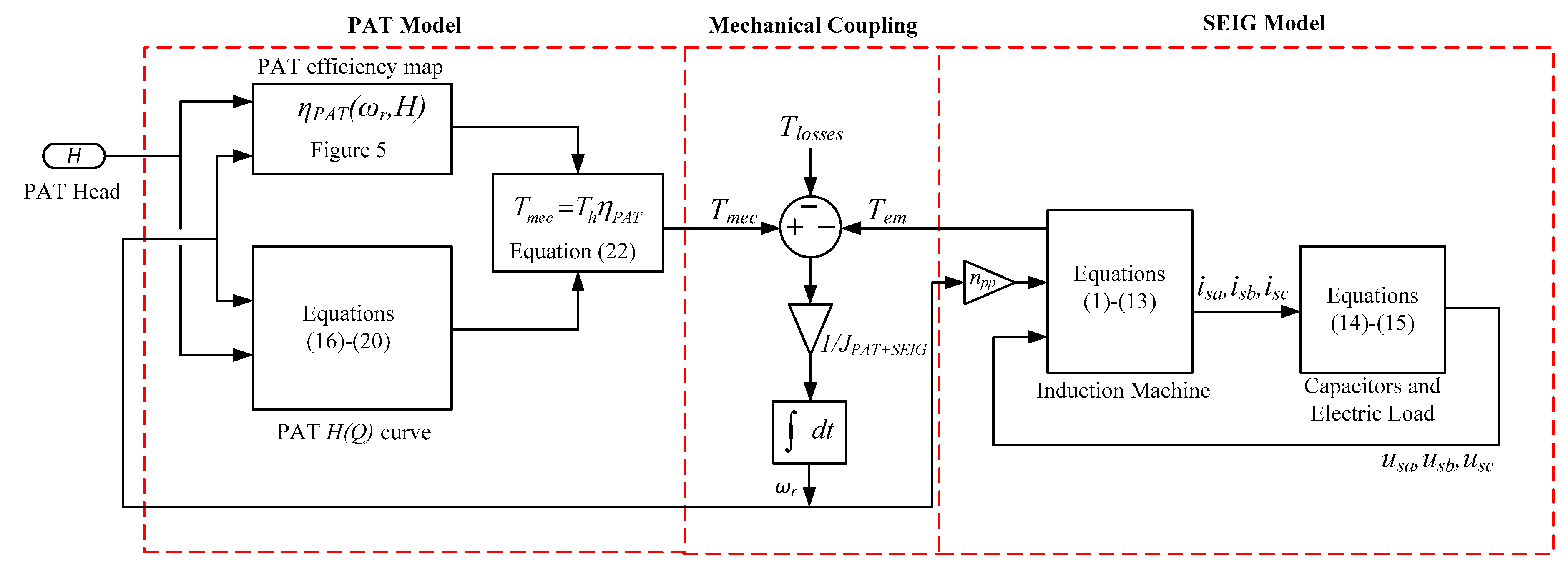
3. Pump as a Turbine (PAT) Model

The pump as a turbine (PAT) model was also developed to couple with the SEIG model. The PAT model was based on the experimental curves obtained in [2,5], which were obtained for different speeds and hydraulic power. In these works, the relation between head and flow were acquired for different turbine speeds. The PAT characteristic curve can be defined by (16), according to [4,8,16], where H is the recovered head in meters water column (m w.c.), Q is the flow in l/s and A, B, and C are non-dimensional coefficients, which depend on the machine characteristics.

$$H \left(m w.c.\right)=A+BQ+C{Q}^2$$

(16)

In this case, the used machine was Etanorm 32-125 KSB. The calibrated characteristic curve is defined by Equation (17) [5]:

$$H \left(m w.c.\right)=3.66-694.45\mathrm{Q}+314560{\mathrm{Q}}^2$$

(17)

To obtain the new characteristic curves when the rotational speed changes, the affinity laws can be used, according to (18) [17], where $\alpha$ is the ratio between rotational speed $N_r$ and the nominal rotational speed ($N_{ref}$). In this research, the $N_{ref}=1050 \mathrm{rpm}$.

$$H={\alpha }^{2}A+\alpha BQ+C{Q}^2$$

(18)

Therefore, the used head curve to develop the hydraulic model was defined by (19), where $\alpha$ can be any value from 0.4 to 1.2. This range was defined considering the possibility of using the similarity laws [16]. Out of this range, the analytical model based on similarity laws, which defines the operational curve, may incur high deviations.

$$H={\alpha }^{2}3.66-\alpha 694.45Q+314560Q^2$$

(19)

The PAT efficiency, ${\eta }_{PAT}$, was also estimated using experimental results obtained in [2]. Figure 5 shows the efficiency surface using a linear interpolation of the experimental points for different operational points and rotational speeds.

The PAT was modeled through two main relations: its efficiency mapping is a function of PAT rotational speed and head curve (see Figure 5), and the Equation (19) to compute the flow as a function of the PAT head and its rotational speed. Considering the differential pressure (dP_rh) imposed by the differential pressure tanks to the PAT terminals (PS1-PS2 in Figure 1), the PAT head can be computed using (20), where $\rho$ is the water density (1000 kg/m³) and $g$ is the standard acceleration due to gravity (9.81 m/s).

$$H=\frac{d{P}_{rh}}{\rho g}$$

(20)

Based on the head and SEIG-PAT speed, ${\omega }_r$, (resulting from the interaction between the PAT, SEIG, capacitors and electrical load), the hydraulic and mechanical torque, $T_h$ and $T_{mec}$ can be computed using (21) and (22), respectively.

$$P_h=\rho gHQ,\hspace{1em}{T}_h=P_h/{\omega }_r$$

(21)

$$P_{mec}=P_h{\eta }_{PAT},\hspace{1em}{T}_{mec}=P_{mec}/{\omega }_r$$

(22)

Figure 6 shows the block diagram of the PAT model. At this point, it should be noted that the PAT model does not include the modeling of the water pipe system and the existing flow control tank, as shown in Figure 1. Therefore, the transient hydraulic dynamics related to the water circulation in the conveyance circuit and its effects on the PAT were neglected, since this analysis was developed in [17,18].

Finally, the connection between the SEIG and PAT systems are represented through the dynamic mechanical Equations (23) and (24), where $T_{losses}$ correspond only to the experimental values obtained for the friction and windage losses in SEIG. The overall diagram of the PAT-SEIG system is shown in Figure 7. The model inputs are the PAT head (H) and the values of the balanced resistive three-phase load and the capacitor bank.

$$J_{PAT+SEIG}\frac{d{\omega }_r}{dt}=T_{mec}-T_{em}-T_{losses}$$

(23)

$$T_{losses}=1.05\times {10}^{-5}{N}_r$$

(24)

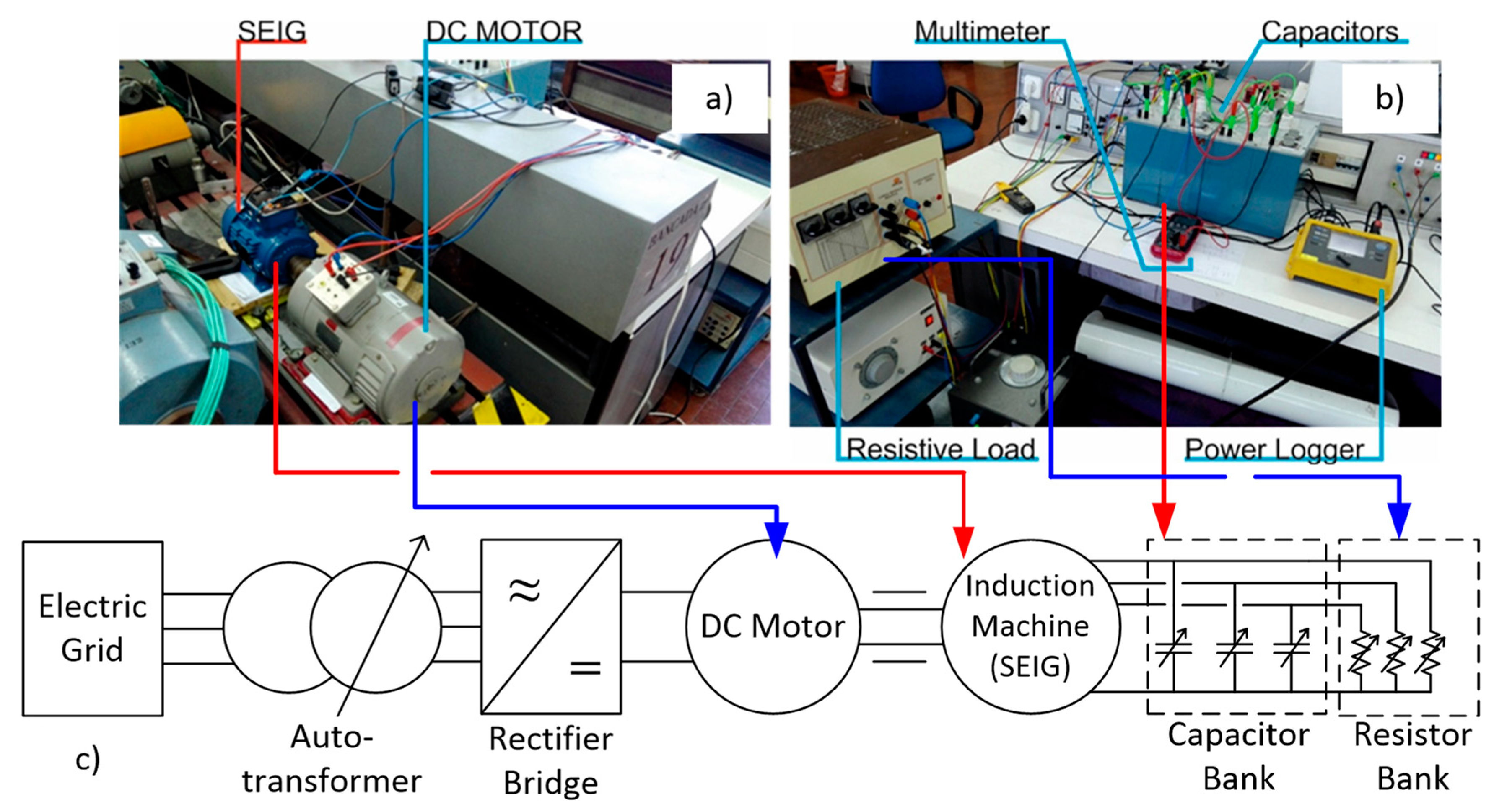
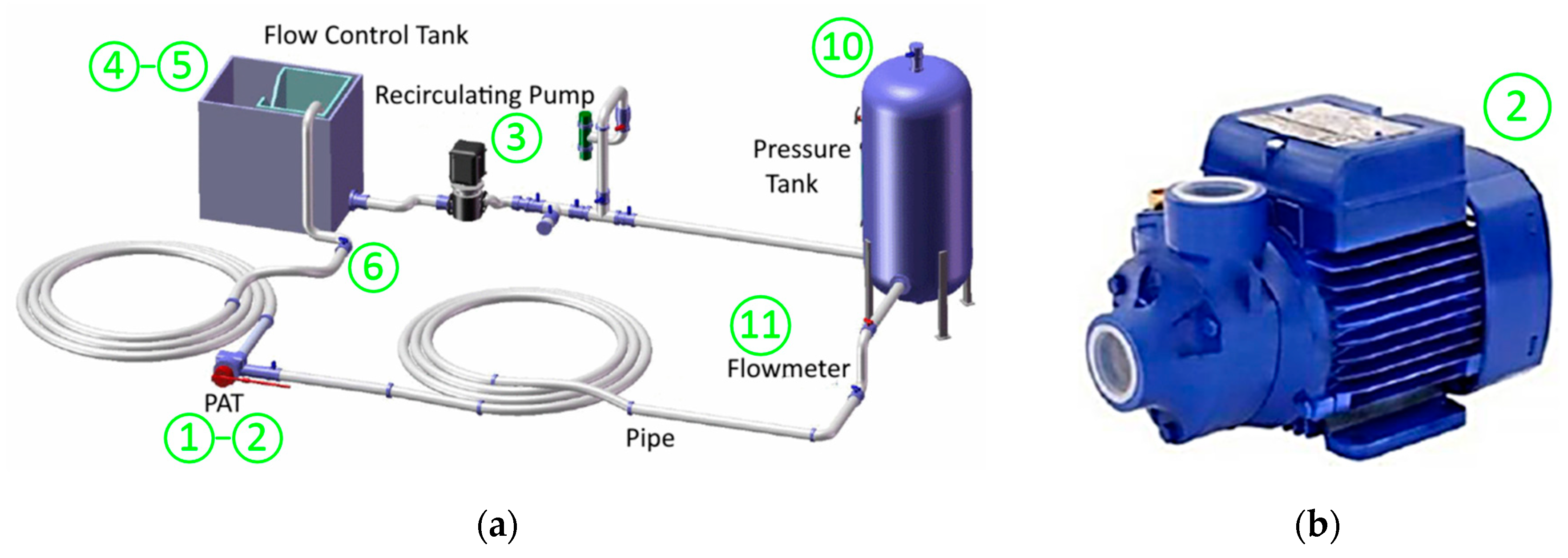
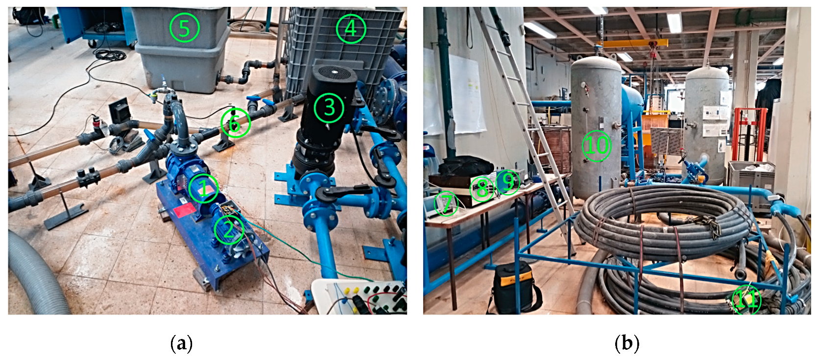
4. PAT-SEIG Model Validation

To validate the developed model, experimental setups were built. The error analysis between simulated and experimental data was done using different error indexes. In this research, to evaluate the fitness of the proposed model, four indicators were proposed:

• I1. Nash–Sutcliffe index (NSI). This index is a fit indicator, which is used in temporal series. NSI value oscillates between −$\infty$ and 1. When values are below 0, the fit is considered poor. When the values are above 0, the model is considered good.

  Table 1. Classification of best fit, according to [19,20].

  Goodness Fit	NSI	RRSE	BIAS
  Very Good	NSI > 0.6	0.00 ≤ RRSE ≤ 0.50	$\mathrm{BIAS}<\pm 0.10$
  Good	0.40 < NSI ≤ 0.60	0.50 < RRSE ≤ 0.60	$\pm 0.10\le \mathrm{BIAS}<\pm 0.15$
  Satisfactory	0.20 < NSI ≤ 0.40	0.60 < RRSE ≤ 0.70	$\pm 0.15\le \mathrm{BIAS}<\pm 0.25$
  Unsatisfactory	NSI < 0.20	RRSE > 0.70	$\mathrm{BIAS}>\pm 0.25$

  shows the used ranges to define the fit according to NSI values. NSI is defined by (25) where $E_i$ is the experimental value in each interval, ${\overline{E}}_i$ is the average of the observed values and $S_i$ is the simulated value in each interval.

  $$NSI=1-\frac{{\sum }_{i=1}^N{\left[E_i-S_i\right]}^2}{{\sum }_{i=1}^N{\left[E_i-{\overline{E}}_i\right]}^2}$$

  (25)
• I2. Root Relative squared error (RRSE). It measures the error of the model by normalizing the variable. Perfect fits are defined when the RRSE value is zero. The efficiency of the simulation is better when the RRSE value is low. This index is defined by (26).

  $$RRSE=\sqrt{\frac{{\sum }_{i=1}^N{\left[E_i-S_i\right]}^2}{{\sum }_{i=1}^N{\left[E_i-{\overline{E}}_i\right]}^2}}$$

  (26)
• I3. Mean relative deviation (MRD). The index defines the significance of the error concerning variable value (27). The fit is good when MRD has values close to 0.

  $$MRD={\displaystyle \sum }_1^x\frac{\left|O_i-P_i\right|/P_i}{x}$$

  (27)
• I4. Bias (BIAS). This index compares the tendency of the simulated values, determining if the simulated values are lower or higher than experimental data (28). The model overestimates if BIAS is negative. When BIAS is positive, the variable is underestimated by the model. The optimal value is zero when BIAS is analyzed.

  $$BIAS=\frac{{\sum }_{i=1}^N{\left[O_i-P_i\right]}^{}}{{\sum }_{i=1}^N{\left[O_i\right]}^{}}$$

  (28)

Table 1 shows the range values defining the goodness of the model when NSI, RRSE and BIAS are considered. These indexes were classified in very good, good, satisfactory, and unsatisfactory. The main indexes to measure the goodness of the model are the NSI, RRSE, and BIAS, according to [19,20]. The MRD value does not have a defined range for each classification. However, it provides additional information about the relative deviation between experimental and simulation results.

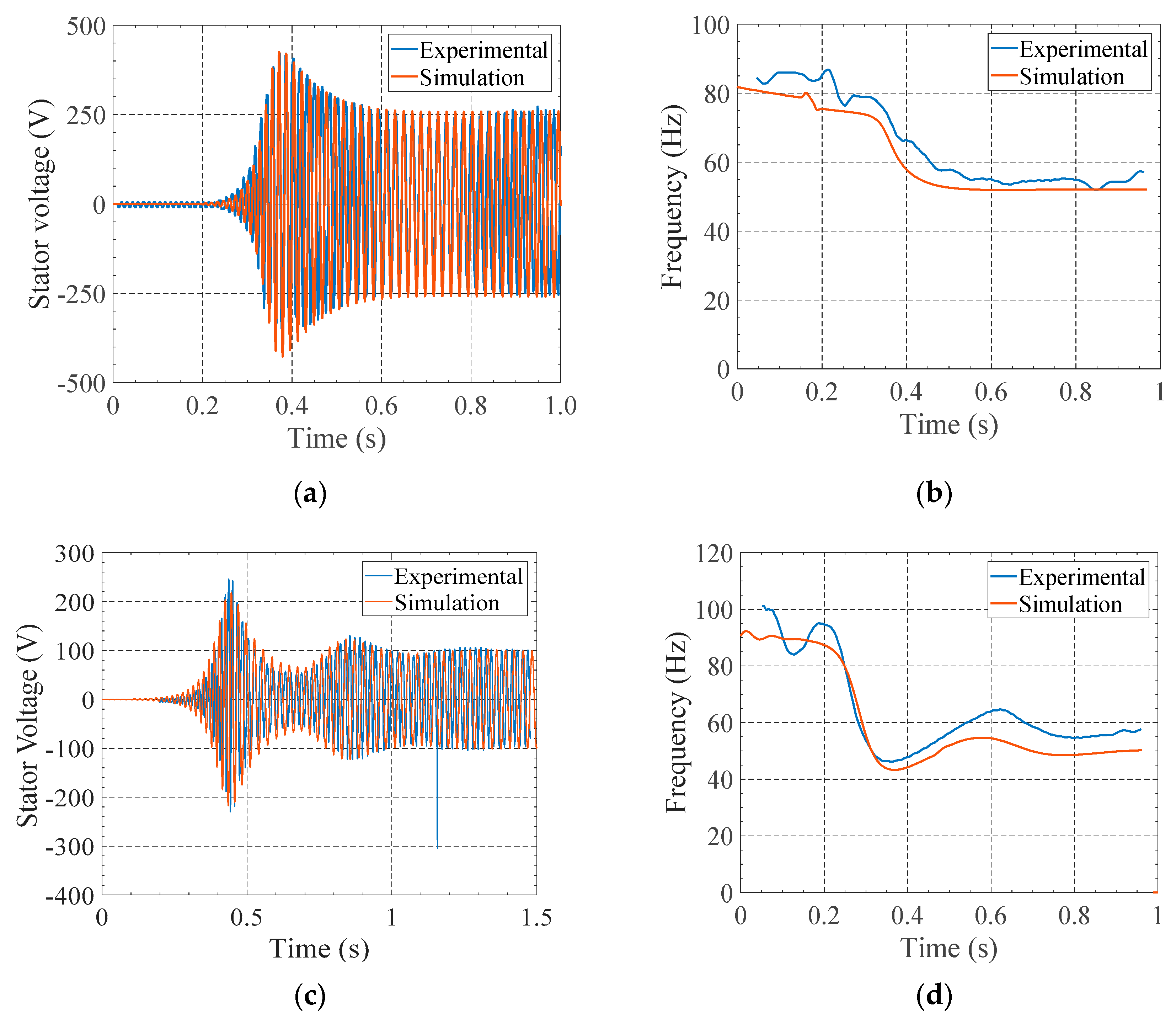
4.1. Self-Excited Induction Generator: d–q Model Validation

Experimental tests were done to validate the d–q SEIG model under steady-state and transient conditions. For this, an experimental setup was developed in the Electrical Machines laboratory at Instituto Superior Técnico (IST), consisting of the SEIG driven by a DC motor, to impose the SEIG external torque, and a resistive electric load.

Figure 8 shows the “wye” squirrel-cage induction machine used as SEIG. Its rated values are listed in

Table 2. Nameplate data of the squirrel-cage induction machine used as SEIG.

Frequency	50 Hz
Voltage	400 V
Current	1.6 A
Output Power	0.55 kW
Power factor	0.73
Speed	910 rpm

. The rated power and efficiency are $P_N$ = 0.55 kW and ${\eta }_N$ = 68%, being its nominal slip, $s_N$, equal to 9%. Figure 9 shows the experimental setup. It is composed by two components. An electromechanical component associated with a DC motor coupled mechanically to the SEIG to act as an external torque source to the generator (Figure 9a) and an electric circuit component made by the variable capacitor and resistor banks, being both connected in parallel to the stator coils of the induction generator (Figure 9b). A general overview of the two experimental setup components is shown in Figure 9c. It shows the electric grid connected to an auto-transformer, which feeds the armature of the DC separated-excitation motor by a diode bridge rectifier. The DC machine is rigidly connected to the induction generator that feeds a capacitor and variable resistive bank.

The first series of tests were done to validate the transient dynamics of the induction generator during its initial self-excitation. Without the capacitor bank and resistive load, the generator is accelerated to a constant reference speed. During this operating condition and without the capacitor bank connected, the generator stator voltage is the remnant one, as indicated in Figure 3, for a speed of $N_r=830$ rpm, $u_{rem}{}_{rms}=0.71$ V. Next, the capacitor bank is connected to begin the self-excitation process. Figure 10 shows the experimental (blue line) and simulated (red line) stator voltage results of the SEIG excitation process using two different capacitor bank values: (a) C = 50 μF and (b) C = 80 μF. Simulation results were obtained using the SEIG model developed in Section 2 (Figure 2). To replicate the laboratorial conditions, the SEIG model was simulated with an external mechanical load applied to its axis (provided from a DC motor, as seen in Figure 9). This was achieved using a similar model to the one shown in Figure 7, where the PAT was replaced by a DC motor torque-speed characteristic ($T_{dc}=k_{\varnothing }\left(U_{dc}-k_{\varnothing }{\omega }_r\right)/R_a$, with $k_{\varnothing }$ and $R_a$ equal to 1.05 and 1.6 Ω, respectively). Without capacitors to excite the induction generator, the DC motor torque was adjusted to meet the initial speed conditions, $N_r$, of each experimental test. After reaching steady state, the capacitors values are added to starting the self-excitation process of the generator. Figure 10 shows the stator voltage in one phase of the SEIG during the excitation process for two different capacitor values: C = 50 μF in Figure 10a and C = 80 μF in Figure 10b.

After the establishment of the SEIG stator voltage, power losses occur inside the machine. These are composed mainly by the stator windings and rotor bars losses, $P_J$, plus the magnetic core losses, $P_{core}$. The windings and rotor bars losses are due to the current injection from the capacitors to the SEIG, being the rotor bars losses caused by the induced rotor currents derived from the electromotive forces produced by the rotating magnetic field which is originated from the currents injected by the capacitor bank. Magnetic core losses are due to the rotating magnetic field created inside the SEIG. Therefore, from the mechanical point of view, the SEIG will demand a higher mechanical torque related to these losses, and thus, after the excitation, the SEIG speed decreases. The initial speed of the SEIG was 830 rpm (before excitation), and the final ones were 750 and 597 rpm (after excitation), respectively.

These error values were analyzed for these figures (Figure 10a,b) according to NSI, RRSE, MRD, and BIAS. These error indexes were described in Section 4 of this research. If stator voltage is analyzed when the capacitance was 50 μF, a very good fit was reached, according to Table 1. In this case, NSI, RRSE and BIAS were 0.955, 0.212 and 0.07, respectively. When the stator voltage was analyzed for a capacitance of 80 μF, the best fit was also very good, with NSI 0.93, RRSE 0.264, and BIAS 0.0357. Therefore, the developed model to simulate the self-excitation process can be considered correct. The deviations between experimental and simulation results are less than 0.044 (4.4% in absolute) for the final steady-state values (

Table 3. Experimental and model steady-state values after the excitation process.

		Experimental	Model	MRD
C = 50 μF	N (rpm)	750	758	+0.010 (1.0%)
	$f_s$ (Hz)	35.2	35.0	−0.006 (0.6%)
	$U_s$ (Vrms)	144	145	+0.007 (0.7%)
C = 80 μF	N (rpm)	597	603	+0.010 (1.0%)
	$f_s$ (Hz)	27.6	27.2	−0.015 (1.5%)
	$U_s$ (Vrms)	113	108	−0.044 (4.4%)

).

Once the validation of the self-excitation dynamic process was developed, the SEIG response to a change of electrical load needs to be analyzed. The same DC motor-SEIG model was used, now to simulate the behavior of the SEIG after a connecting of resistive load. The simulation was done in two steps: first, the SEIG was excited without electrical load and, after reaching a steady-state condition, the resistive load is connected. Figure 11 and Figure 12 show the experimental and simulation results of the SEIG: (a) stator voltage, (b) stator current, (c) active power, (d) reactive power, and (e) magnetizing flux; after connecting an R_L of 600 Ω and 300 Ω, respectively. These resistive loads mimic an electric demand to the SEIG from a consumer. Since in the experimental setup, a DC motor provides the SEIG mechanical torque, its speed decreases with the increase of electric load. Notice that this is similar behavior to the PAT. When decreasing the resistive load, the electric current increases and, if the stator voltage remains (or has a very small change), the requested active power $P_a=3\frac{U_s{}^2}{R_L}$ would increase. However, Figure 11 shows that this is not true. When the requested active power increases, the speed of the DC motor decreases and thus also the SEIG electrical frequency and stator voltage. Decreasing the stator voltage will also decrease the stator current, Figure 11a,b, decreasing the active power, Figure 11c, and increasing the machine’s speed. Also, a reduction of electrical frequency will influence the reactive power, as shown in Figure 11d, provided by the capacitor to the SEIG, thus changing the SEIG operation point, per Figure 11e. In conclusion, this process will be iterative until a new steady state is obtained. The SEIG starts without electric load, with a capacitor bank of C = 35 μF, and the current at its rated value, I = 1.6 Arms. After the inclusion of the resistive load, $R_L$ = 600 Ω, the rms stator voltage and current drop, from 183 Vrms to 141 Vrms and from 1.6 Arms to 1.05 Arms, Figure 11a,b, respectively. This is due to the reduction of speed, N, and electrical frequency, $f_s$, resulting into new active and reactive powers, shown in Figure 11c,d, and a new magnetizing flux inside the machine, $E/f$, shown in Figure 11e. As shown in

Table 4. Comparison between steady-state experimental and model’s results after the application of resistive loads.

		Experimental		Model		MRD
		Initial	Final	Initial	Final	Initial	Final
$R_L$ = 600 Ω	N (rpm)	839	834	842	835	+0.004 (+0.4%)	+0.001 (+0.1%)
	$f_s$ (Hz)	41.0	40.0	40.9	39.3	−0.000 (−0.0%)	−0.018 (−1.8%)
	$U_s$ (Vrms)	183	141	191	141.9	−0.044 (−4.4%)	−0.006 (−0.6%)
	$I_s$ (Arms)	1.6	1.05	1.53	1.12	−0.023 (−2.3%)	+0.023 (+2.3%)
	$E/f$ (V${\mathrm{Hz}}^{-1}$)	4.46	3.53	4.67	3.61	−0.005 (−0.5%)	+0.003 (+0.3%)
$R_L$ = 300 Ω	N (rpm)	848	843	849	851	+0.001 (0.1%)	+0.010 (+1.0%)
	$f_s$ (Hz)	41.2	40.3	41.5	40.0	+0.007 (+0.7%)	−0.007 (−0.7%)
	$U_s$ (Vrms)	181	90	184.6	84.8	+0.002 (+0.2%)	+0.058 (+5.8%)
	$I_s$ (Arms)	1.6	0.8	1.62	0.87	+0.013 (+1.3%)	+0.088 (+8.8%)
	$E/f$ (V${\mathrm{Hz}}^{-1}$)	4.4	2.2	4.49	2.22	+0.020 (+2.0%)	+0.009 (+0.9%)

, MRDs between the simulation and experimental results are less than 0.088 (8.8%). The highest deviation of 0.088 occurs for low magnetization points of the SEIG, $E/f$ = 2.2. This is related to the magnetizing inductance, $L_M$, obtained experimentally. For lower values of magnetic flux, the stator leakage cannot be neglected and, thus, the associated error to the determination of $L_M$ increases.

These errors were estimated to measure the goodness of fit. When the errors were calculated to the stator voltage (Figure 11a), the values of NSI, RRSE and BIAS were 0.629, 0.609 and −0.0434, respectively, reaching very good values for NSI and BIAS, and good for RRSE. Similar values were got when the stator current was analyzed between experimental and simulated values. Very goodness fit was reached for three indicators (NSI [0.687], RRSE [0.386] and BIAS [0.0105]). Excellent values were reached when active and reactive power were analyzed. The NSI, RRSE, and BIAS were 0.964, 0.189 and 0.055, respectively, for the active power. In contrast, the values were 0.933 (NSI), 0.258 (RRSE) and 0.0281 (BIAS) for the reactive power. Finally, when the magnetizing flux was studied, the values of NSI, RRSE, and BIAS were 0.784, 0.138, and −0.0317, respectively. Therefore, a very good fit was reached in this model when the SEIG was compared, connecting a resistive load equal to 600 Ω.

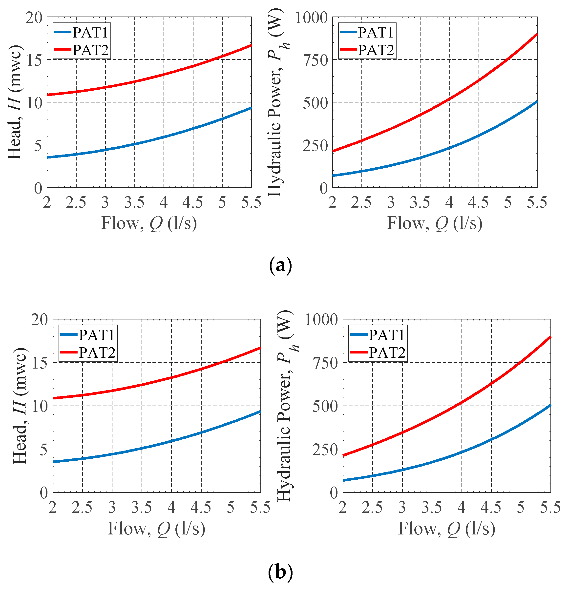
4.2. PAT Model Validation

A second set of experimental tests was performed to validate the PAT model represented by the PAT model in Figure 6. Figure 13a,b shows a scheme of the hydraulic circuit used with the PAT installed. The hydraulic circuit is composed of a pressure tank to constant guaranty pressure applied to the radial PAT and an Etanorm 32-125 KSB 4.8 PAT. This machine (PAT1) had a nominal rotational speed of 1020 rpm and a rated flow of 4.2 L/s, a flow control tank to eliminate possible turbulences in the hydraulic circuit, and a recirculating pump to close the hydraulic circuit. The specific speed was 51 rpm (m, kW), and the best efficiency point (BEP) was defined in the operation point 3.36 L/s and 4 m w.c. Figure 14 shows the experimental setup assembled at the laboratory (IST). Figure 14a highlights the PAT (1), the induction generator (2), the recirculating pump (3), the control flow tanks (4-5), and the pressure transducer (6). In Figure 14b, one highlights the measurement and the oscilloscope (7), the resistive load bank (8), the capacitor bank (9), the pressure tank (10), and the flowmeter (11).

A set of experimental tests were done to validate the PAT model in steady-state and transient conditions. Simulation results were now obtained using the PAT-SEIG model in Figure 7. Models’ inputs are the PAT head and the values of the resistive load and capacitors. All simulations start with a non-excited SEIG to obtain the PAT steady-state for a set of initial conditions. After reaching the steady-state hydraulic conditions, the capacitors are added to the SEIG to start with its excitation process, with and without a resistive load. Following the new steady-state conditions of the PAT-SEIG system (with and without resistive load), a sudden change of resistive load is applied to the SEIG, and the new transient behavior can be analyzed.

Starting without the capacitor bank and at no-load, a differential head of 5.82 m w.c. was applied to the PAT’s terminals, regulating the air vessel (Figure 14b element 10) to guarantee a uniform head value. After the establishment of the PAT steady-state conditions, the excitation capacitor bank was showing a value of 17.4 μF connected to the no-load SEIG to start its excitation process, as shown in Figure 15a,b. It shows the evolution of the no-load SEIG stator voltage and the electric frequency (experimental and simulation) until the magnetic saturation of the induction generator limited it, stabilizing around 250 V and 55 Hz. To verify the affection of the electric load in the excitation process, the previous starting process was repeated. In this case, an electrical load equal to 300 Ω was connected. The capacitor bank value was varied from C = 17.4 μF to C = 34.7 μF to guaranty the excitation of the induction generator. The results of this experimental test are shown in Figure 15c,d. When these figures are observed, the time to excite the SEIG increases when it starts with an electrical load and presents an oscillatory transient. Therefore, the best methodology is to start first the excitation without electrical load and to connect the electrical load only after the SEIG voltage is stabilized. If a comparison is developed, the analytical approximation is really good. It is confirmed when the errors are considered (

Table 5. Error analysis for the compared variables.

Indexes	Stator Voltage (Figure 15a)	Frequency (Figure 15b)	Stator Voltage (Figure 15c)	Frequency (Figure 15d)
NSI	0.960 (VG)	0.797 (VG)	0.802 (VG)	0.841 (VG)
RRSE	0.200 (VG)	0.451 (VG)	0.441 (VG)	0.399 (VG)
BIAS	0.039 (VG)	−0.071 (VG)	0.095 (VG)	−0.075 (VG)
MRD	−0.0244 (−2.44%)	0.062 (6.2%)	0.010 (1.0%)	0.0664 (6.64%)

(VG.—Very Good; G.—Good; S.—Satisfactory; P.—Poor).

). These show a very good fit for all analyzed errors applied to all variables. Therefore, the model correctly reproduced the behavior of the PAT-SEIG model.

Once the validation of the excitation process was developed, two additional tests were performed to verify the accuracy of the PAT-SEIG coupled models under transient conditions. After exciting the SEIG, a sudden change of electrical load or capacitor bank was applied to the PAT-SEIG system. Figure 16a,b shows the stator voltage and electric frequency transient behaviors before and after a reduction of the electric load. The PAT-SEIG system started with $R_L$ = 600 Ω, C = 17.4 μF and $H$ = 7.5 m w.c. When the establishment of the SEIG steady-state was around 170 V of amplitude (120.2 Vrms), the electric load was decreased to $R_L$ = 300 Ω at 0.1s. With a lower resistance, the SEIG stator voltage drops, performing an oscillatory transient to the new steady-state regime around 130 V of amplitude (92 Vrms).

In Figure 16c,d, the load remained at $R_L$ = 300 Ω but an increase of the capacitor bank value was applied to the PAT-SEIG system at around 0.22 s. The PAT-SEIG started considering a C value of 17.4 μF, and it was increased to 34.7 μF. An overvoltage is seen in the SEIG stator voltage from 120 V to around 190 V, and a reduction of the electric frequency occurs from 58 Hz to 40 Hz.

In all tests, the simulation results follow the experimental ones. To measure the errors between them and to calibrate the model, the errors were defined as well as the goodness of fit.

Table 6. Error indexes for the compared variables.

Indexes	Stator Voltage (Figure 16a)	Frequency (Figure 16b)	Stator Voltage (Figure 16c)	Frequency (Figure 16d)
NSI	0.569 (G)	0.787 (VG)	0.761 (VG)	0.793 (VG)
RRSE	0.648 (S)	0.462 (VG)	0.429 (VG)	0.455 (VG)
BIAS	0.063 (VG)	−0.041 (VG)	−0.034 (VG)	−0.037 (VG)
MRD	0.0360	0.0269	−0.054	0.281

(VG.—Very Good; G.—Good; S.—Satisfactory; P.—Poor).

shows a very good fit for all analyzed parameters. The error was very good in all analyses for different parameters, except for the stator voltage. For this parameter, the values were good and satisfactory when the NSI and RRSE were determined. The obtained values showed that the analytical model could be used in other hydraulic and electrical conditions, such as when these recovery systems operate in serial or parallel. MRD also showed satisfactory values since MRD values are under 0.1 (10%).

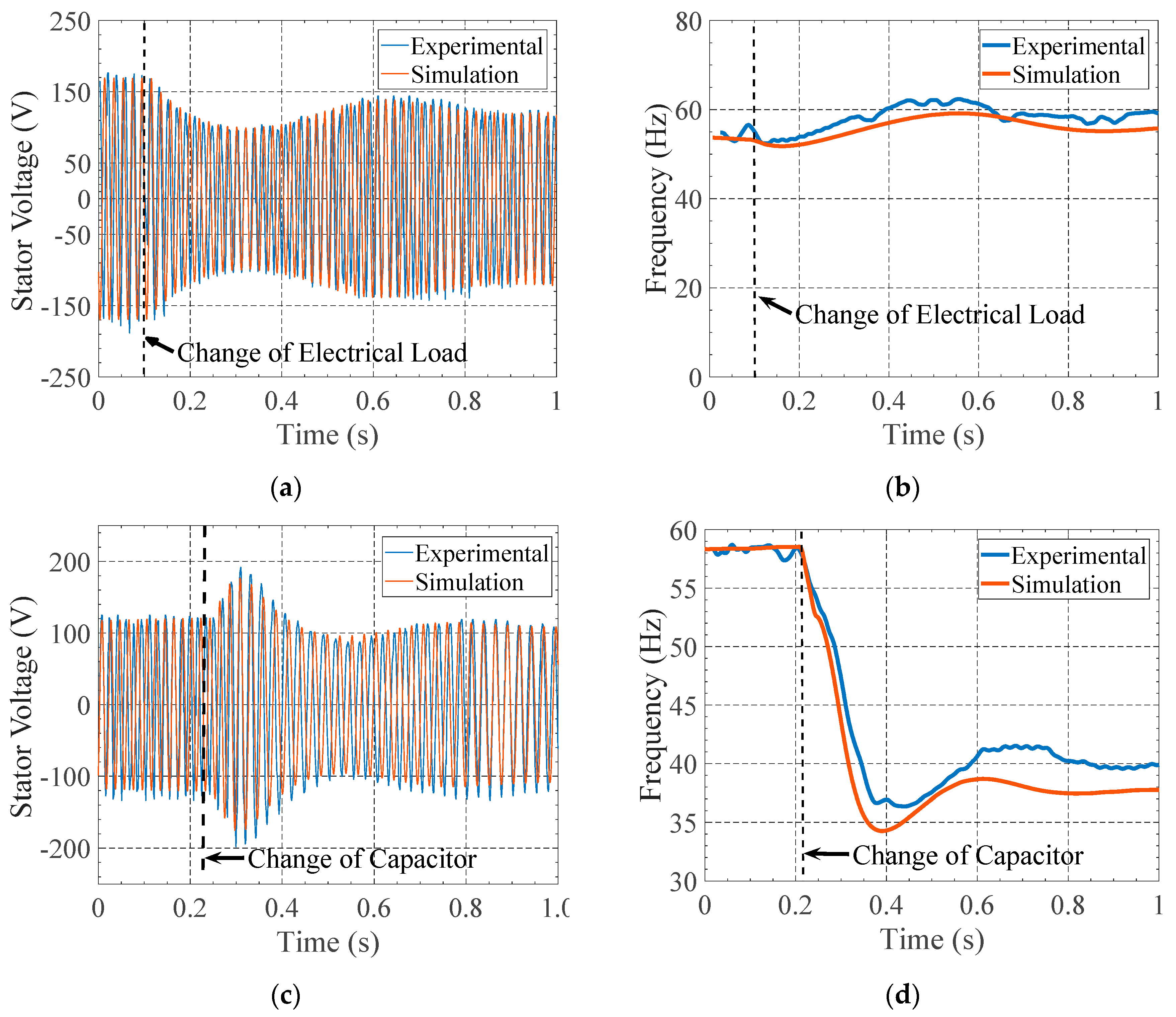
5. Impact of Electric and Hydraulic Perturbations in the PAT-SEIG Stability

The PAT-SEIG system is a complex hydraulic-electromechanical non-linear system, which has a high number of variables. These variables change over time rapidly, and this variation depends on the hydraulic and electric constraints (i.e., flow, head, electric load and capacitor value). The transient dynamics of the whole system results from the interaction behaviors of both PAT and SEIG subsystems. This means that a small sudden change in an electrical variable may influence the hydraulic one and vice-versa. In this section, a sudden change of electrical or hydraulic parameters is analyzed to show how this affects the system operation after reaching a steady-state condition. The tested scenarios consider sudden variations of (1) the value of the capacitor bank, (2) the resistive load, and (3) the hydraulic pressure.

Due to the limitation of the Hydraulic lab conditions in terms of the air-vessel and PAT hydraulic power, the SEIG was not able to reach its rated power within the tested range of speeds. Therefore, for simulation purposes, the PAT curve ($H \mathrm{vs}. Q$) was reallocated to higher head values, as shown in Figure 17. This allows higher hydraulic power within the same range of speeds. The new proposal PAT was defined by the characteristic curve (29).

$$H \left(m w.c.\right)=10.99-694.45\mathrm{Q}+314560{\mathrm{Q}}^2$$

(29)

Figure 17 shows the hydraulic curves (H vs. Q and P_h vs. Q) for the original PAT (PAT1 in blue) and the new one (PAT2 in red). PAT2 is now able to produce enough hydraulic power to set the SEIG rated conditions (rated power of 550 W). The specific speed of PAT2 was 20 rpm (m,kW), and the best efficiency point (BEP) was defined in the operation point 3.48 L/s and 12.38 m w.c.

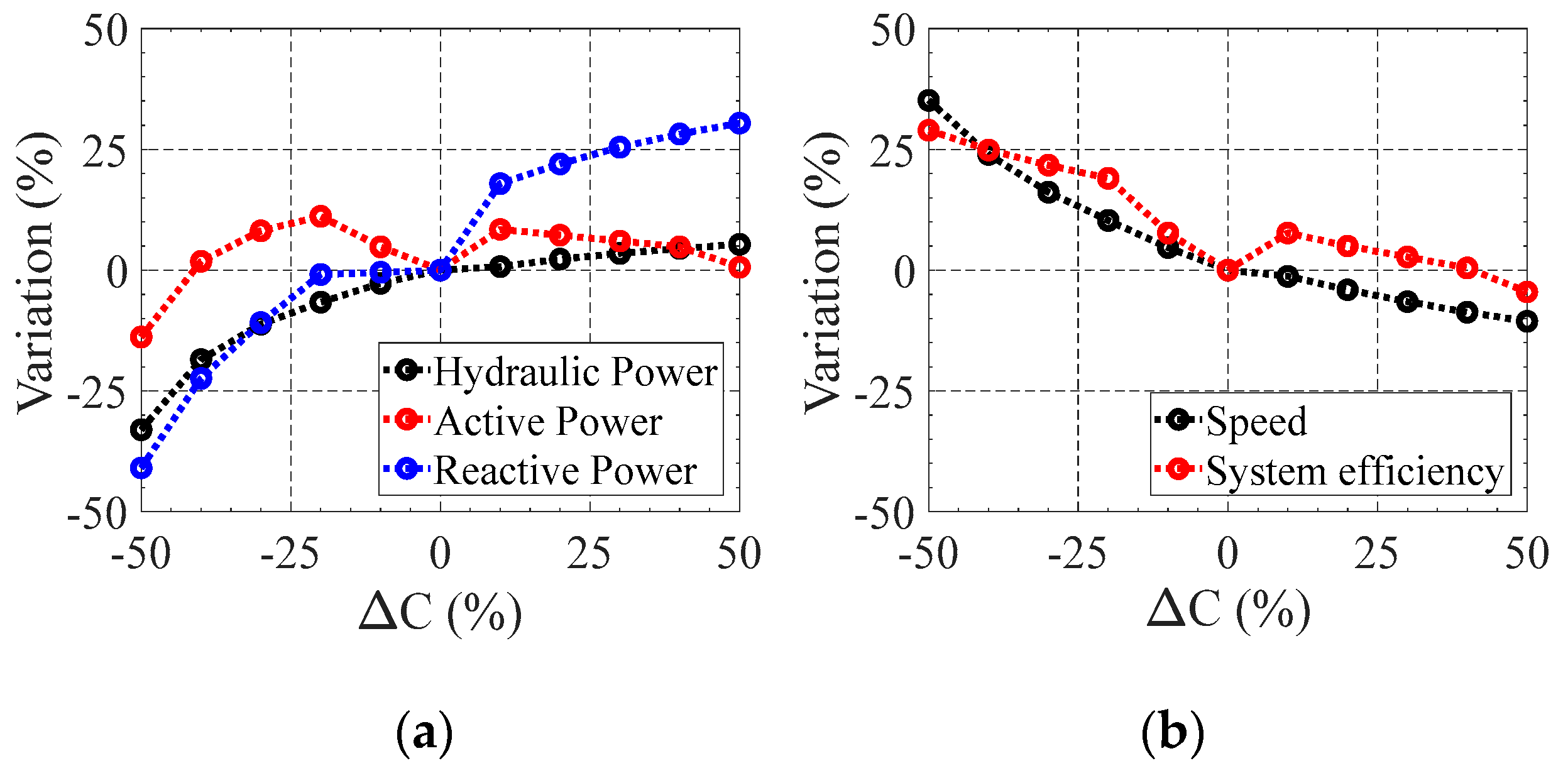
5.1. Variation of Excitation Capacitance

The first set of tests applied a sudden change in the excitation capacitor values, with the PAT-SEIG system already excited and under steady-state conditions. The initial steady-state conditions were reached for a differential PAT head, $∆H$, of 21.5 m w.c., an initial capacitor value, C_i, of 35 μF and an electric load of $R_L$ = 200 Ω. Next, the capacitors’ value was changed, and the new steady-state electromechanical and hydraulic conditions were recorded.

Table 7. Steady-state hydraulic and electromechanical quantities after a sudden change in the capacitors’ value.

$\mathsf{∆}$C.	${\mathit{P}}_{\mathit{h}} \left(\mathbf{W}\right)$	N (rpm)	${\mathit{U}}_{\mathit{s}}{}_{\mathit{r}\mathit{m}\mathit{s}} \left(\mathbf{V}\right)$	${\mathit{I}}_{\mathit{s}}{}_{\mathit{r}\mathit{m}\mathit{s}} \left(\mathbf{A}\right)$	${\mathit{P}}_{\mathit{a}} \left(\mathbf{W}\right)$	${\mathit{Q}}_{\mathit{r}} \left(\mathbf{Var}\right)$	${\mathit{\eta }}_{\mathit{s}\mathit{y}\mathit{s}}$
−50%	1005	1365	139.7	1.16	331	−392	33.0%
−40%	1223	1252	152.6	1.34	392	−515	32.0%
−30%	1333	1173	157.4	1.47	416	−592	31.1%
−20%	1401	1114	158.8	1.58	427	−658	30.5%
−10%	1460	1057	155.5	1.60	403	−661	27.6%
0%	1501	1010	150.2	1.65	384	−664	25.6%
+10%	1512	997	157.0	1.83	417	−783	27.6%
+20%	1535	969	155.2	1.90	412	−810	26.9%
+30%	1553	944	154.4	1.95	408	−833	26.3%
+40%	1568	922	152.1	2.01	403	−851	25.7%
+50%	1581	903	149.4	2.07	387	−866	24.4%

shows the final steady-state hydraulic and electric parameters after a sudden change of the capacitor’s value.

In this table, $∆$C is the applied variation of the capacitors in (%), $P_h$ is the resultant hydraulic power, N the PAT-SEIG speed, $U_s{}_{rms}$ and $I_s{}_{rms}$ are the SEIG stator voltage and current rms values, $P_a$ and $Q_r$ are the SEIG active and reactive power, and ${\eta }_{sys}$ is the PAT-SEIG overall achieved efficiency. Note that the negative value in $Q$ indicates that the reactive power is flowing from the capacitors to the SEIG.

Figure 18 is also possible to visualize the variation of the hydraulic, active and reactive powers and the system speed and efficiency. It is possible to observe that decreasing the capacitors’ value increases the system speed and efficiency. This follows the results obtained in [2,5], where an inverse relationship between the speed and capacitors’ values was obtained. The active power (red line in Figure 18a) provided from the SEIG shows a slight $\pm 15\%$ change of its value for the capacitor’s variation between −50% and +50%. In contrast, the reactive one (blue line) follows the variation of the capacitors. Due to mainly reactive power, the SEIG magnetic and windings losses decrease with the reduction of capacitors (red line in Figure 18b), thus requesting lower values of hydraulic power from the PAT for lower values of C. This shows that it is possible to control the PAT hydraulic power from changing the capacitor values in the SEIG.

Another important aspect is the behavior of the SEIG stator current with the variation of capacitors. Increasing the capacitors’ value increased the SEIG current. This can lead to an overload state of the SEIG that, if not considered, may significantly decrease the generator’s lifetime and/or damages it due to overheating of its electric insulation.

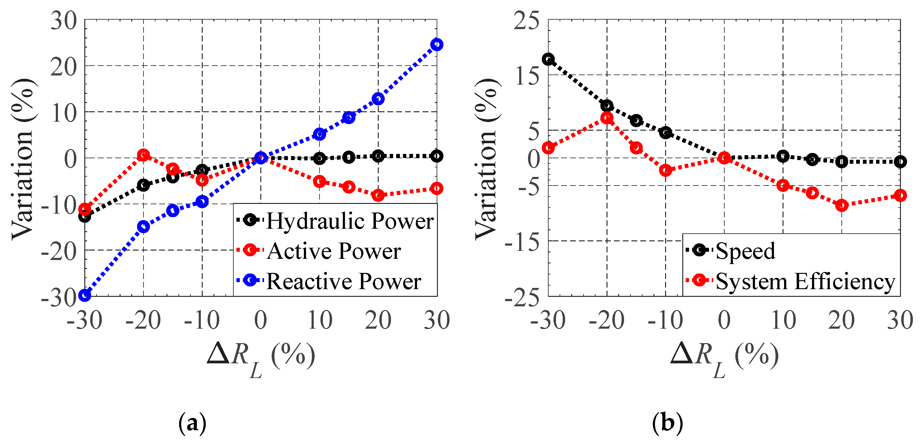
5.2. Variation of Resistive Load

The same study was done regarding a sudden change of the resistive load. Equal initial steady-state conditions were considered using a differential PAT head, $H$, of 21.5 m w.c., a capacitor value, C, of 35 μF and an initial electric load of $R_{Li}$ = 200 Ω. After reaching steady-state, a sudden change in the electrical resistance was applied.

Results in

Table 8. Steady-state hydraulic and electromechanical parameters after a sudden change in the resistance value.

$\mathsf{∆}{\mathit{R}}_{\mathit{L}}$	${\mathit{P}}_{\mathit{h}} \left(\mathbf{W}\right)$	N (rpm)	${\mathit{U}}_{\mathit{s}}{}_{\mathit{r}\mathit{m}\mathit{s}} \left(\mathbf{V}\right)$	${\mathit{I}}_{\mathit{s}}{}_{\mathit{r}\mathit{m}\mathit{s}} \left(\mathbf{A}\right)$	${\mathit{P}}_{\mathit{a}} \left(\mathbf{W}\right)$	${\mathit{Q}}_{\mathit{r}} \left(\mathbf{Var}\right)$	${\mathit{\eta }}_{\mathit{s}\mathit{y}\mathit{s}}$
−30%	1311	1190	119.1	1.54	342	−466	26.1%
−20%	1412	1105	135.6	1.61	387	−565	27.5%
−15%	1439	1078	139.6	1.60	375	−588	26.0%
−10%	1460	1056	141.5	1.60	366	−601	25.0%
0%	1501	1010	150.2	1.65	384	−664	25.6%
+10%	1499	1013	153.5	1.66	365	−698	24.3%
+15%	1503	1007	157.9	1.66	360	−722	24.0%
+20%	1507	1003	159.2	1.69	353	−749	23.4%
+30%	1507	1003	168.1	1.75	359	−827	23.9%

and Figure 19 show that the change of SEIG’s resistive load highly influences the SEIG stator voltage and reactive power. Being the capacitor bank in parallel to the SEIG stator terminals, both share the same voltage. Therefore, a decrease of SEIG’s terminal voltage implies a decrease of reactive power stored at the capacitor bank. Despite the reactive evolution, the active power remains almost unchanged with the electric resistance, presenting a slight increase with the decrease of the resistance. For $∆R_L$ = −30%, the SEIG starts losing its excitation, getting near to its non-excited zone. The speed and PAT-SEIG system efficiency have similar behavior with the variation of the electrical resistance: they both decrease with the increase of the electric resistance. This is in agreement with the behaviors of the hydraulic, reactive and active power. Despite the active power remaining almost constant, with the increase of the reactive power, the magnetic power losses inside the SEIG increases, thus resulting in a decrease of the SEIG efficiency.

Another important aspect is the evolution of the current. When decreasing the electric resistance, the current presents a slow reduction. However, with the increase of the resistance, the current presents a higher increase. This must be taken into consideration, as an increase of the SEIG current to values higher than its nominal one, which may damage the SEIG in a medium or long term.

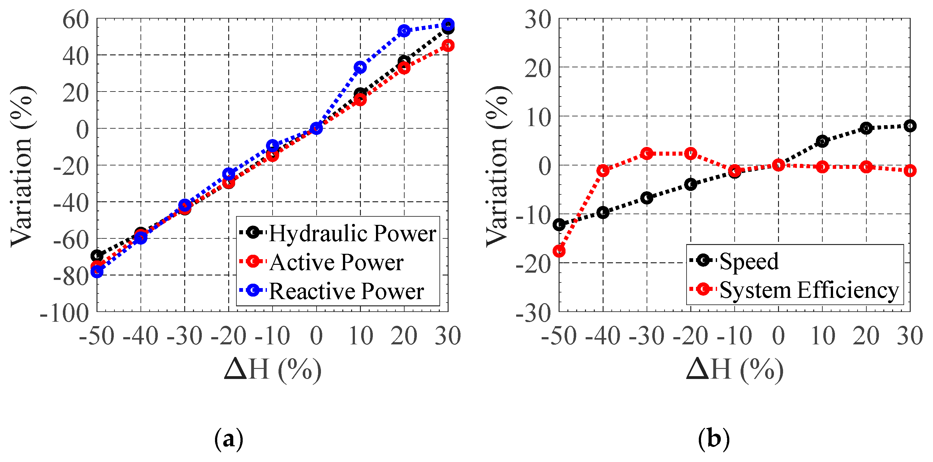
5.3. PAT Head Variation

The PAT head variation ($∆H$) is an important issue, as it is common to occur in industrial applications due to external influences. This case analyzed the impact of a sudden increase or decrease of the PAT head in the overall PAT-SEIG operation. The same initial steady-state conditions were considered with an initial differential PAT head, $H_i$, of 21.5 m w.c., a capacitor value, C, of 35 μF and an electric load of $R_L$ = 200 Ω.

Results presented in Figure 20 and

Table 9. Steady-state hydraulic and electromechanical quantities after a sudden change in the PAT head

$\mathsf{∆}\mathit{H}$	${\mathit{P}}_{\mathit{h}} \left(\mathbf{W}\right)$	N (rpm)	${\mathit{U}}_{\mathit{s}}{}_{\mathit{r}\mathit{m}\mathit{s}} \left(\mathbf{V}\right)$	${\mathit{I}}_{\mathit{s}}{}_{\mathit{r}\mathit{m}\mathit{s}} \left(\mathbf{A}\right)$	${\mathit{P}}_{\mathit{a}} \left(\mathbf{W}\right)$	${\mathit{Q}}_{\mathit{r}} \left(\mathbf{Var}\right)$	${\mathit{\eta }}_{\mathit{s}\mathit{y}\mathit{s}}$
−50%	457	887	75.0	0.74	96	−145	21.1%
−40%	642	912	100.2	1.01	163	−267	25.3%
−30%	842	942	118.8	1.23	221	−386	26.2%
−20%	1057	970	132.9	1.41	277	−499	26.2%
−10%	1297	995	144.8	1.55	334	−601	25.3%
0%	1501	1010	150.2	1.65	384	−664	25.6%
+10%	1782	1059	170.2	1.92	453	−885	25.5%
+20%	2047	1086	180.6	2.08	521	−1017	25.5%
+30%	2320	1091	181.3	2.11	569	−1040	25.3%

shows there is a linear behavior of the hydraulic, active and reactive power and rotational speed with the variation of PAT head. Regarding the system efficiency, results indicated that only in an extreme case characterized by a significant decrease of head pressure (−50%) would the PAT-SEIG suffer a meaningful reduction of its efficiency. Another important effect is the increase of SEIG current with the PAT head, which may damage the SEIG if the current exceeds its rated value.

6. Conclusions

The study of the improvement of sustainable indicators in water systems has been an important issue in this last decade, especially in the context of sustainable development goals for 2030. The improvement of the efficiency in water systems can be leveraged by using PATs, which have been mainly studied in the last years under the hydraulic point of view. However, the PATs analysis cannot only be focused on hydraulic behavior, as PAT requires an electrical machine to operate. In the particular case of off-grid (absence of electrical grid) applications, using self-excited induction generators, the hydraulic-electric behavior becomes more complex.

This research focuses on delving into the study of the hydraulic-electrical transient stability interaction when possible perturbations occur in an off-grid PAT-SEIG system. Analytical models were developed to simulate the PAT and the SEIG behaviors, both individually validated through experimental tests. Then the coupled PAT-SEIG model also validated experimentally in IST hydraulic laboratory, was tested for different electrical loads. To analyze the accuracy of the models, error measures were considered, resulting in NSI values between 0.75 and 0.98 and BIAS values below 0.10.

The developed models can estimate the variation in SEIG voltage, current and frequency, as well as in the PAT flow and recovered head when a sudden change in the resistive load, capacitance and PAT head occurs. With a sudden increase of resistive load, the hydraulic power and SEIG stator current remain almost constant. However, there is an increase of the SEIG reactive power and a decrease in the PAT-SEIG efficiency. With a sudden increase of the SEIG capacitors or PAT head, the SEIG stator current increases and PAT-SEIG efficiency decreases. The increase of the SEIG current may be critical, as it may contribute to the machine overload.

The possibility to estimate these variations will allow operators to define new operating models, in which new recovery systems can be coupled between them. This analytical coupling will measure the injected perturbations in the water grid or electrical batteries when the electric and the hydraulic transients occur. These developed models are the basis for the real integration of the PATs in the water sector, where they can correctly operate under hydraulic and/or electric regulation conditions. The use of these models can be extrapolated to other off-grid electro-hydraulic systems, considering both electrical and hydraulic parameters of the used machines.

References

1. Postacchini, M.; Darvini, G.; Finizio, F.; Pelagalli, L.; Soldini, L.; di Giuseppe, E. Hydropower generation through pump as turbine: Experimental study and potential application to small-scale WDN. Water 2020, 12, 958. [Google Scholar] [CrossRef] [Green Version]
2. Capelo, B.; Pérez-Sánchez, M.; Fernandes, J.F.P.; Ramos, H.M.; López-Jiménez, P.A.; Branco, P.J.C. Electrical behaviour of the pump working as turbine in off grid operation. Appl. Energy 2017, 208, 302–311. [Google Scholar] [CrossRef]
3. Fecarotta, O.; Aricò, C.; Carravetta, A.; Martino, R.; Ramos, H.M. Hydropower potential in water distribution networks: Pressure control by PATs. Water Resour. Manag. 2014, 29, 699–714. [Google Scholar] [CrossRef]
4. Ramos, H.; Borga, A. Pumps as turbines: An unconventional solution to energy production. Urban Water 1999, 1, 261–263. [Google Scholar] [CrossRef]
5. Fernandes, J.F.P.; Pérez-Sánchez, M.; Silva, F.F.; López-Jiménez, P.A.; Ramos, H.M.; Branco, P.J.C. Optimal energy efficiency of isolated PAT systems by SEIG excitation tuning. Energy Convers. Manag. 2019, 183, 391–405. [Google Scholar] [CrossRef]
6. Yi, Y.; Zhang, Z.; Chen, D.; Zhou, R.; Patelli, E.; Tolo, S. State feedback predictive control for nonlinear hydro-turbine governing system. J. Vib. Control 2018, 24, 4945–4959. [Google Scholar] [CrossRef]
7. Khan, M.F.; Khan, M.R. Analysis of voltage build-up and speed disturbance ride-through capability of a self-excited induction generator for renewable energy application. Int. J. Power Energy Convers. 2016, 6, 157–177. [Google Scholar] [CrossRef]
8. Carravetta, A.; del Giudice, G.; Fecarotta, O.; Ramos, H. PAT design strategy for energy recovery in water distribution networks by electrical regulation. Energies 2013, 6, 411–424. [Google Scholar] [CrossRef] [Green Version]
9. Morani, M.C.; Carravetta, A.; del Giudice, G.; McNabola, A.; Fecarotta, O. A comparison of energy recovery by pATs against direct variable speed pumping in water distribution networks. Fluids 2018, 3, 41. [Google Scholar] [CrossRef] [Green Version]
10. Liu, Y.; Tan, L. Tip clearance on pressure fluctuation intensity and vortex characteristic of a mixed flow pump as turbine at pump mode. Renew. Energy 2018, 129, 606–615. [Google Scholar] [CrossRef]
11. Liu, Y.; Tan, L. Symmetrical and unsymmetrical tip clearances on cavitation performance and radial force of a mixed flow pump as turbine at pump mode. Renew. Energy 2018, 127, 368–376. [Google Scholar]
12. Han, Y.; Tan, L. Dynamic mode decomposition and reconstruction of tip leakage vortex in a mixed flow pump as turbine at pump mode. Renew. Energy 2020, 155, 725–734. [Google Scholar] [CrossRef]
13. Pérez-Sánchez, M.; Sánchez-Romero, F.J.; López-Jiménez, P.A.; Ramos, H.M. PATs selection towards sustainability in irrigation networks: Simulated annealing as a water management tool. Renew. Energy 2018, 116, 234–249. [Google Scholar] [CrossRef]
14. García, I.F.; Nabola, A.M. Maximizing hydropower generation in gravity water distribution networks: Determining the optimal location and number of pumps as turbines. J. Water Resour. Plan. Manag. 2020, 146, 04019066. [Google Scholar] [CrossRef]
15. Simões, M.G.; Farret, F.A. Modeling and Analysis with Induction Generators, 3rd ed.; CRC Press: Boca Raton, FL, USA, 2014; ISBN 9781482244670. [Google Scholar]
16. Mataix, C. Turbomáquinas Hidráulicas; Universidad Pontificia Comillas: Madrid, Spain, 2009. [Google Scholar]
17. Pérez-Sánchez, M.; López-Jiménez, P.A.; Ramos, H.M. PATs operating in water networks under unsteady flow conditions: Control valve manoeuvre and overspeed effect. Water 2018, 10, 529. [Google Scholar] [CrossRef] [Green Version]
18. Carravetta, A.; Houreh, S.D.; Ramos, H.M. Pumps as Turbines, Fundamentals and Applications; Springer: Cham, Switzerland, 2018. [Google Scholar] [CrossRef]
19. Pérez-Sánchez, M.; Sánchez-Romero, F.J.; Ramos, H.M.; López-Jiménez, P.A. Calibrating a flow model in an irrigation network: Case study in Alicante, Spain. Span. J. Agric. Res. 2017, 15, e1202. [Google Scholar] [CrossRef]
20. Moriasi, B.; Arnold, J.; van Liew, M.; Binger, R.; Harmel, R.; Veith, T. Model evaluation guidelines for systematic quantification of accuracy in watershed simulations. Trans. ASABE 2007, 50, 885–900. [Google Scholar] [CrossRef]
Figure 1. PAT+SEIG scheme. Hydraulic and electrical circuit.
Energies 13 04521 g001
Figure 2. SEIG model block diagram.
Energies 13 04521 g002
Figure 3. Induced remnant voltage of the induction machine for different rotational speeds.
Energies 13 04521 g003
Figure 4. Connection between induction machine, capacitors and resistive load.
Energies 13 04521 g004
Figure 5. PAT efficiency experimental curve.
Energies 13 04521 g005
Figure 6. PAT model.
Energies 13 04521 g006
Figure 7. SEIG-PAT model.
Energies 13 04521 g007
Figure 8. Squirrel-cage induction machine used as SEIG.
Energies 13 04521 g008
Figure 9. Experimental setup to test the SEIG, isolated from the PAT: (a) DC motor coupled mechanically to the SEIG, (b) variable capacitor and resistor banks both connected in parallel to the stator coils of the induction generator, (c) scheme of two experimental setup components.
Energies 13 04521 g009
Figure 10. SEIG stator voltage during the excitation process with: (a) C = 50 μF and (b) C = 80 μF. In blue, the experimental results. In red, the simulation ones.
Energies 13 04521 g010
Figure 11. SEIG stator voltage when connecting a resistive load of R L = 600 Ω with the SEIG excited with a capacitor bank having C = 35 μF: (a) stator voltage, (b) stator current, (c) active power, (d) reactive power and (e) magnetizing flux.
Energies 13 04521 g011
Figure 12. SEIG stator voltage when connecting a resistive load of R L = 300 Ω with the SEIG excited with a capacitor bank having C = 35 μF.
Energies 13 04521 g012
Figure 13. Experimental hydraulic circuit: (a) circuit schematic and (b) PAT used (Etanorm 32-125 KSB 4.8).
Energies 13 04521 g013
Figure 14. Experimental hydraulic circuit developed for validation of the PAT model: in (a) the PAT-SEIG, control flow tanks and recirculating pump and, in (b) the pressure tank and the resistive load and capacitors.
Energies 13 04521 g014
Figure 15. PAT-SEIG stator voltage and frequency during excitation with: C = 17.4 μF, R L = Ω and H = 5.82 m w.c: (a) stator voltage and (b) electric frequency; and with C = 34.7 μF, R L = 300 Ω and H = 7.5 m w.c.: (c) stator voltage and (d) electric frequency.
Energies 13 04521 g015
Figure 16. PAT-SEIG stator voltage and electric frequency after a sudden change: (a,b) change of electric load from R L = 600 Ω to R L = 300 Ω, with C = 17.4 μF and H = 7.5 m w.c. and (c,d) change of capacitor from C = 17.4 μF to C = 34.7 μF with R L = 300 Ω and H = 7.5 m.w.c.
Energies 13 04521 g016
Figure 17. Hydraulic characteristic curves of the original PAT (PAT1, blue color) and the new one (PAT2, red color), for N = Nref: (a) head curve and (b) hydraulic power curve.
Energies 13 04521 g017
Figure 18. Variation of hydraulic and electromechanical quantities after a change in the capacitor, C: (a) variation of hydraulic (black), active (red) and reactive (blue) powers, and (b) variation of speed (black) and system (red) efficiency.
Energies 13 04521 g018
Figure 19. Variation of hydraulic and electromechanical parameters after a change in the resistive load, R L : (a) variation of hydraulic (black), active (red) and reactive (blue) powers, and (b) variation of speed (black) and system (red) efficiency.
Energies 13 04521 g019
Figure 20. Variation of hydraulic and electromechanical parameters after a change in the PAT head, H : (a) variation of hydraulic (black), active (red) and reactive (blue) powers, and (b) variation of speed (black) and system (red) efficiency.
Energies 13 04521 g020