Abstract
Bioenergy has been globally recognized as one of the sustainable alternatives to fossil fuels. An assured supply of biomass feedstocks is a crucial bottleneck for the bioenergy industry emanating from uncertainties in land-use changes and future prices. Analytical approaches deriving from geographical information systems (GIS)-based analysis, mathematical modeling, optimization analyses, and empirical techniques have been widely used to evaluate the potential for bioenergy feedstock. In this study, we propose a three-phase methodology integrating fuzzy logic, network optimization, and ecosystem services assessment to estimate potential bioenergy supply. The fuzzy logic analysis uses multiple spatial criteria to identify suitable biomass cultivating regions. We extract spatial information based on favorable conditions and potential constraints, such as developed urban areas and croplands. Further, the network analysis uses the road network and existing biorefineries to evaluate feedstock production locations. Our analysis extends previous studies by incorporating biodiversity and ecologically sensitive areas into the analysis, as well as incorporating ecosystem service benefits as an additional driver for adoption, ensuring that biomass cultivation will minimize the negative consequences of large-scale land-use change. We apply the concept of assessing the potential for switchgrass-based bioenergy in Missouri to the proposed methodology.
1. Introduction
Bioenergy has been recognized as one of the sustainable alternatives to fossil fuels, and the quantification of bioenergy potential is an essential field of research. The design of the biomass supply chain is a major stumbling block for bioenergy and includes three spatially interlinked elements, including (i) resource assessment, (ii) logistic planning, and (iii) biorefinery design [1]. Perennial biomass crops, such as switchgrass (Panicum virgatum L.), face adoption challenges owing to the considerable time required to establish the plant and uncertainties associated with land-use change and price fluctuations [2,3,4]. However, an inadequate volume of potential biomass feedstocks also presents a barrier; Richard et al. suggested that ethanol production at the commercial level is challenged by the low density of biomass feedstock across the landscape [5,6]. This situation has led investments in the bioenergy industry to be described as a chicken-and-egg problem, wherein investment in feedstock processing and fuel production is not forthcoming due to uncertainty in feedstock supply, while farmers are simultaneously unwilling to cultivate dedicated bioenergy feedstocks as there is no assured demand for the product [7]. However, development of renewable energy sources has been mandated by the U.S. government, and cellulosic-based production has been subjected to substantial interest by the U.S. Department of Energy (DOE) and the Department of Agriculture (USDA). In 2005, it was estimated that the cellulosic-based biofuel industry would require about 342 × 106 Mg of domestic perennial biomass to produce the necessary quantity of bioethanol for the US [8]. However, only about 10,216 Mg of herbaceous biomass has been produced annually in the USA, as documented in the 2016 Billion-Tons Report [9]. Under the renewable fuel standard (RFS) program, a statutory volume of 10.5 billion gallons cellulosic biofuel was proposed, however, only 0.59 billion gallons (5.6%) were produced [10].
Analytical approaches based on geographical information systems (GIS), mathematical optimization, and empirical techniques have been used to evaluate the potential for bioenergy feedstock cultivation and its ensuing impacts on land-use change, the feedstock processing industry, and sustainability across various parts of the world. The economic viability and performance of bioenergy production largely hinge on the location of the biomass processing facility relative to supply, as it has significant ramifications on resource availability, logistic cost, and sustainability [1]. Significant research has been done in solving the issue of co-locating a diffuse feedstock with a refinery. In one of the earlier examples, Voivontas et al. introduced a spatial distribution method assessing biomass potential by a four-level analysis based on technological and economically exploitable potential agricultural residues on the island of Crete [11]. In this methodology, a GIS decision support system explored possible restrictions and candidate power plants to estimate the needed cultivation area for biomass collection. Advancing on predecessors, Beccali et al. estimated the technical and economic potential for woody residues and energy crops for Sicily using a GIS-based methodology, including data on land cover, terrain elevation, climate, precipitation, and geological features [12]. Höhn et al., determined potential biomass and sites for biogas plants in Southern Finland using a kernel density (KD) map to pinpoint areas with high biomass concentration for conversion and exploitation [13]. Based on the KD analyses’ results, biogas candidate sites were assigned using a network location-allocation solver in the ArcGIS platform, which minimizes the sum of all weighted distances between biomass sources and facilities using p-median algorithm [13,14,15]. Sultana et al., furthered these methods by using fuzzy logic to develop a land suitability model for biomass-based facility development in an analytic hierarchy process (AHP) to combine environmental criteria and contrasted that lack of straightforward valuation methods [14]. These studies assessed the bioenergy potential based on the existing biomass sources and optimized the transportation routes from these sources to bioenergy facilities.
Several studies have suggested that growing perennial herbaceous crops on marginal land has the potential for high potential yield with low investment costs [4,16,17,18]. However, these publications do not answer questions of scale, which are essential for the development of a viable industry. Also, there is no strict definition of marginal land [19]; some studies defined marginal lands as “lands that are not suitable for food-based agriculture and have limited economic potential for fulfilling other ecosystem services” [20], while others stated that marginal land includes vacant and abandoned lands, degraded lands, and poor agricultural potential lands [21,22]. As such, the use of marginal lands for crop cultivation may not be practical as a policy solution. These studies, however, did not assess the potential ecosystem impacts of projected land-use change for large scale biomass cultivation on the regional environment.
In this study, we integrated fuzzy logic and network optimization to assess potential bioenergy supply and used ecosystem service evaluation to validate our choices for land cover transitions. Feedstock accessibility was evaluated based on potential crop yield and the cost of transportation to existing biorefineries. Fuzzy logic analysis using multiple input criteria, including climatic conditions, soil types, and topography, was used to identify ideal areas for biomass cultivation and harvest. Additional constraints, such as developed urban areas, infrastructure, and traditional food crop zones, were used to further narrow the available landmass. To minimize negative externalities from bioenergy crop transitions, we integrated an ecosystem service assessment based on the known values for switchgrass land cover. Our analysis extends prior studies by incorporating biodiversity and ecologically sensitive areas into the fuzzy logic analysis, ensuring that biomass cultivation will minimize negative consequences of large-scale land-use change and how these changes impact ecosystem services relating to carbon sequestration, annual water yield, and soil erosion. We apply the following conceptual framework (Figure 1) to assess the potential for switchgrass-based bioenergy in Missouri.
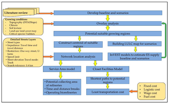
Figure 1.
Conceptual research framework.
2. Materials and Methods
2.1. Methods
The current study assesses bioenergy potential for biomass cultivation and spatial optimization of existing bioenergy facilities. Figure 1 illustrates the conceptual model structures used in this research. In the first step of this method, we applied multiple-criteria spatial factors (including environmental and socioeconomic) to locate suitable regions for growing energy crops. These spatial factors were described as geospatial rasters (30 m resolution) and transformed into binary images by reclassifying cells within the favored areas by “1” and cells outside the area by “0”. These reclassified layers were then used as input data to a fuzzy overlay model which is expressed by the following equation [14]:
where was the value of the i-th cell in the final overlay maps; was the Boolean value (0,1) assigned for the i-th cell in the j-th input layers; n is the number of factors considered in the study.
We reclassified the collected data of both preferred and constraint factors to create discrete variables based on the selected growing conditions. The reclassified layer was used as an input for the overlay analysis by combining favorable conditions for all variables using the “AND” combination method [23]. As such, if a location was identified as suitable under all data layers, then it would be classified as suitable. Consequently, if any aspects/variables were unsuitable, the entire cell was determined to be unsuitable. Therefore, our assessment represents a conservative estimate of suitable growing areas on which a bioenergy crop could be produced. We used the land use/cover raster to build scenarios by changing land use/cover attributes. For example, scenarios could be based on using marginal land for growing the crop in the research region, or land use/cover scenarios can be modified based on available conditions.
In the second phase, the study utilizes network location and sensitivity analyses to identify transportation frameworks to optimize logistics and supply chain aspects of biomass delivery. The network analysis is based on Dijkstra’s algorithm to find the single-source, shortest-path connecting two nodes (a source and a destination) in a weighted graph G = (V, E), where V is a set of vertices or elements, including nodes, junctions, or intersections in a road network, and E is a set of directed edges or road segments that connect ordered pairs of vertices in V. The weight or cost of transport can be travel time and/or travel distance. The algorithm builds a set S of vertices, S ϵ V, which includes the final smallest weight w from the determined source s. Noting that w is the weight of an ordered pair (u, v) ϵ E, the algorithm repeatedly finds the vertex u ϵ V–S, adds u to S, and relaxes all edges different than u [24]. In this methodology, by placing the existing biorefinery at the center of assigned service areas as determined sources, s, we identify the potential biomass supply region for each refinery based on minimum distance computations. The outcome of the network location analyses is a set S of potential cultivation areas that connect to the biorefineries by the shortest paths. The ArcGIS Network Analyst extension is executed to achieve this step.
To estimate the feedstock area of existing bioethanol refineries, we used the Service-Area solver to create concentric serviced regions that encompass all open streets within a specified impedance. To estimate optimized transportation paths used to calculate the costs of transportation of biomass delivery, we applied Closet-Facility solver in the ArcGIS platform, which minimizes the distance from individual incidents and existing local biorefineries to their potential biomass sources. By doing this, we determined viability at each of these plants, though resources may not be allocated evenly, as many of these plants may not have sufficient supply depending on the scenario. We assumed that trucks depart from biorefineries to collect feedstock from potential areas identified through fuzzy logic analysis. We used two break conditions: break time and break distance for a professional truck driver [15]. This option allowed areas that do not have direct road access to be considered in the analysis. In both Service-Area and Closest-Facilities solvers, the impedances were travel time and travel distance. The Facilities-To-Find was set with the existing local biorefineries, while the Location-Type for both potential sites and facilities was established with an either-side-of-vehicle approaching type, to prevent the vehicles from having to approach from only one side of the road. The Search-Tolerance for street map features was 1.6 km (1-mile) to make sure that all the potential elements were captured. We assigned the Global-Turns to generate turn restrictions; the study assumed that all vehicles are allowed to perform U-turns only at intersections and dead-ends and that all potential sites and facilities could be approached from either side of the vehicle [15,22]
Biomass transportation cost ($. Mg−1) is often calculated as a sum of total time cost and total distance transportation cost. While time cost accounts for the capital cost of the truck and labor cost, the distance transportation cost accounts for a fully loaded truck traveling to the facility and for empty trucks on the backhaul [9]. In this study, we calculated the transportation cost using the equation below (Equation (2) [9,25]).
where L, logistic cost, is the cost for loading and unloading biomass from a purpose-built bale truck, T, travel time (minutes) is time for a truck collecting biomass to travel both to and from the facility. This value is an output of Closest-Facility solver, while wage cost, W, is the average regional wage of a truck driver ($ per minute), fuel cost, F, is the average regional cost for fuel consumed during biomass transportation. Fixed cost, FC, is an average cost that represents vehicle maintenance, replacement cost, and other upkeep costs.
X = L + T × (W + F + FC)
Finally, we performed a sensitivity analysis by applying Monte Carlo simulation to identify possible outcomes and probabilities the transport cost will occur based on uncertainties of cost parameters.
2.2. Case Study
For the case study of growing switchgrass (Panicum virgatum L.) in Missouri, we located areas that are most suitable for switchgrass based on ideal growing conditions including soil type, annual rainfall, seasonal temperature, and the slope of the terrain. Many studies agree that switchgrass is considered as a high potential bioenergy feedstock as it can produce ample biomass, has sizable ethanol conversion potential, is native to the U.S., and can be grown on low-quality lands with limited use of fertilizers [26,27]. Switchgrass provides a range of ecosystem services and has the potential to be an excellent biomass feedstock. Mitchell et al., confirmed that growing switchgrass on marginal soil returned an ethanol yield equal to or higher than that of no-till corn.
The state of Missouri, located in the Midwestern United States, represents a varied landscape that consists of marginal and degraded lands, as well as lands that lie in floodplains, which researchers and policymakers have emphasized as necessary for bioenergy feedstock cultivation. Furthermore, switchgrass has a relatively high yield potential throughout the state of Missouri [28]. We assumed that new cellulosic-based biorefineries would be co-located with the existing ones in order to benefit from existing infrastructure. Six biorefineries are operating in the study region, whose details on location, feedstock, biofuel platform, and biofuel generation capacity can be found in Table 1 [29]. Using the biorefineries’ locations, we created a 128-km (80-mile) buffer, which represents the longest one-way distance that a truck with a long-log trailer can haul biomass feedstocks effectively [25,30,31]. The buffered polygons were merged to generate one unified preliminary area. The final area of interest includes Missouri and neighboring states, including Kansas, Nebraska, Iowa, and Illinois, and covers a total area of 130,612 km2.

Table 1.
Details of Missouri operating biorefineries in the study area including necessary location information as well as current feedstock information and capacity.
We excluded wetlands, conservation regions, the US reservation areas, and developed areas (including street network, urban sections, and pipeline network) from the analysis, as they would be unsuitable for switchgrass cultivation. Our assumptions regarding favorable growing conditions were informed based on published literature. Table 2 lists the details, including values/ranges for specific variables, data types, and references for our assumptions.
Table 2.
Range of favorable climactic and topographic conditions for growing switchgrass.
The data used in this study were selected to represent the environmental conditions that determine feedstock suitability based on availability and economic feasibility of transportation. Spatial soil properties, land use types, road networks, temperature, rainfall, and other relevant inputs were collected in vector and raster format from various sources including geospatial data from the US Department of Agriculture (USDA), US Geological Survey (USGS), and ESRI® Data & Maps. The maximum temperature data for 30 years were extracted from the National Oceanic and Atmospheric Administrator (NOAA) 1981–2010 Climate Normals database. Mean precipitation values were collected from the USDA Natural Resources Conservation Service (NRCS) from 1981–2010 [32]. The land use/cover data were extracted from the National Land Cover Database 2011 [33]. The spatial resolution was maintained at a 30 m resolution for all raster layers during suitable region assessment analyses.
To analyze the potential transportation of switchgrass to biorefineries, we used the 2005 detailed U.S. street map layer to plan routes from refineries to potential fields [34]. While it would be ideal to have a more recent road map, the required richness of data for our method necessitated using an older, but a complete road map.
Terrain slope has essential considerations when evaluating a site for potential agriculture due to difficulties associated with operating farming/harvesting equipment. The slope, in percentage, was represented in a raster using the slope spatial analysis tool in ArcGIS version 10.6. The input data for this tool used a digital elevation model (DEM) raster extracted from National Elevation Data 30m (NED_30m) compiled from USDA/NRCS—National Geospatial Center of Excellence [35].
We collected detailed soil texture data at the county level for the study region. The soil attribute database was downloaded from the Geospatial Data Gateway, USDA [36]. We used Soil Data Viewer 6.2 (SDV 6.2), an ArcGIS compatible toolkit supplied by the Natural Resources Conservation Service, to extract the necessary soil texture shapefiles to categorize data into broad soil-texture types and make our analysis tractable [37]. SDV 6.2 allows one to access soil interpretations and soil properties that are contained within the complex soil database. The SDV 6.2 generated spatial attributes of soil types and displays results as spatial maps. Since all spatial soil texture data at the county level were collected, we merged them and dissolved to create one soil layer. Soils were classified into 11 categories, including loamy sand, silt loam, silty clay loam, clay loam, fine sandy loam, loam, very gravelly silt loam, very gravelly silty clay loam, gravelly silt loam, moderately decomposed plant material, and silty clay [27,37,38,39,40,41].
Falling temperatures can cause lower growth rates and ultimately lower yields. Therefore, we constructed a temperature raster that represented temperatures only during the growing season (May-September). Triangulated irregular network (TIN) interpolation is one of the most popular methods for representing digital models, which is used to estimate missing values of any location-dependent attributes such as precipitation, temperature, or elevation. We used the TIN interpolation tool in QGIS to generate the spatial temperature using monthly data from 150 adjacent national meteorological stations, resulting in a spatial temperature raster [42]. This raster was projected to WGS 1984/UTM Zone 15S and used as one of the inputs for the fuzzy overlay analysis. Critical species habitats, extracted from U.S. Fish & Wildlife Service, ECOS [43], were excluded from the potential area to mitigate unintended consequences.
In the case study, based on the land use/cover classification, we investigated scenario (scenario 1) using marginal lands, which included areas of fallow/idle cropland, barren land, and switchgrass, as classified by Homer et al. [33]. Scenario 2 used marginal lands and non-food cropland for growing switchgrass. The non-food crop was defined as industrial crops, including grass, pasture, alfalfa, hay, and sod/grass seed. Table 3 describes land-use-land-cover (LULC) changes in different scenarios where fallow/idle cropland, alfalfa, grass/pasture, and sod/grass seed are theoretically converted to switchgrass.
Table 3.
LULC class changes in different scenarios. Food crops are unaffected and non-food uses are targeted.
For applying network analyses in the case study, we used a detailed street map, which was extracted from ESRI_DM (2005), clipped to the preliminary potential area, and projected to the WGS 1984/UTM Zone. We used an eleven-hour break time and a break distance of 240 km (150 miles) as requested by the Federal Motor Carrier Safety Administration (FMCSA) for a truck carrying agricultural products [31,53]. We also set a 1.6-km (1-mile) search tolerance, which snapped the facilities to the closest street map features, allowing areas that do not have direct road access to be still considered in the analysis. While the biorefinery location is used as each facility point, a centroid pixel located at the center of the polygon, representing a suitable area, serves as a supply point (an incident) in the network [22]. Figure 2 describes the location and selected factors of the case study in Missouri.
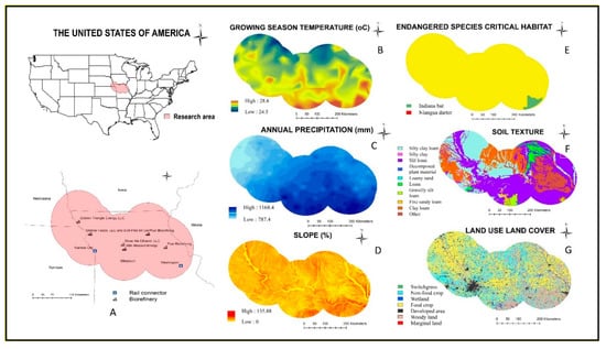
Figure 2.
The location and selected factors of the case study in Missouri: (A) Case study location; (B) Growing season temperature; (C) Annual precipitation; (D) Terrace slope; (E) Critical habitats; (F) Soil texture; (G) Land use land cover.
Although we assumed that switchgrass could replace existing land cover where suitable areas are defined, these changes can cause negative impacts to their ecosystem services. To evaluate these potential impacts, we quantified carbon storage, annual water yield, and overland sedimentation to estimate potential feedbacks of the LULC changes in different scenarios using the Integrated Valuation of Ecosystem Services Tradeoffs (InVEST) 3.8.0 modeling software [54]. The annual water yield, a difference between the annual precipitation and real evapotranspiration, is estimated using the Budkyo curve method. The carbon storage model matches land cover to estimate carbon pools in soil, above-ground and below-ground biomass, and woody debris using a lookup table. The sediment delivery ratio model computes total sediment generated, sediment export, sediment retention using the universal soil loss equation (USLE) combined with a connectivity index [55]. We used LULC maps in three scenarios, including base, scenario 1, and scenario 2, as LULC inputs of models to compare between scenarios. Supplementary Materials describes the InVEST model’s settings in detail.
To calculate transportation costs, we used the values presented in Table 4, and all values are adjusted to 2019 dollars.
Table 4.
Cost of transportation. Including locally normalized costs for loading, unloading and storage per load and ranges for fuel, wages and equipment in the study area.
3. Results
Switchgrass cultivation shows significant promise in the northern region of Missouri. If the entire proposed study areas in scenario 2 were cultivated, it would provide up to 8923 × 106 L of bioethanol at an average transport cost of $8.60 per Mg of switchgrass, or just over $0.16 per liter of ethanol. Also, switchgrass, due to its physiology, could reduce sedimentation by up to 2% and increase the carbon storage in the landscape by 3% by changing only a small portion of the land area. However, scenario 1 shows that at this spatial resolution, marginal land does not provide substantial feedstock for a switchgrass-based industry with current cropping patterns.
3.1. Potential Cultivating Regions of Switchgrass
In scenario 1, where only marginal land, fallow, and idle crops were selected, the suitable area accounted for approximately 4755.6 hectares, equivalent to a 74% increase in current switchgrass plantings. In scenario 2, wherein marginal land and non-food cropland were selected, the suitable area increased significantly to more than 1.7 million hectares, which accounts for upwards of 13.5% of the total study area (Figure 3). There were 116 and 3343 suitable locations found by the fuzzy overlay analysis in scenarios 1 and 2, respectively, that were suitable for switchgrass cultivation. The sizes of parcels were varied widely, ranging from 0.1 ha to 212.6 ha with a median of 9 ha in scenario 1, and 1 ha to 136,992 ha with a median of 150.8 ha in scenario 2. Figure 3 demonstrates the broad range of region sizes between scenarios 1 and 2.
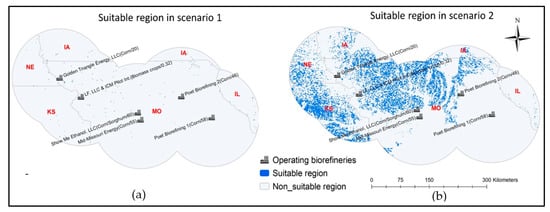
Figure 3.
Suitable switchgrass cultivation. (a) in scenario 1, (b) in scenario 2. The plant name is presented with its feedstock and capacity. State abbreviations are in red.
The dark blue pixels in Figure 3 each represent an aggregation of suitable 900 square meter parcels of land. Each operating biorefinery was shown with its production capacity, in millions of gallons per year (MMgy) and its feedstock type.
3.2. Switchgrass Feedstock Supply Areas
We used the Service-Area analyst to quantify accessibility from facility locations to the surrounding area. In our study, the service area estimated the ability of biorefineries to access their potential switchgrass suppliers by the local road network. Figure 4 presents the Service-Area analyst results. Although the network analyst was set with the maximum 11-h drive time, the results show that a haul truck departing from an existing biorefinery could reach any potential site in the study area within only 180 min, driving one-way. In one hour, the service areas covered about 24.3% and 25.9% of switchgrass suitable regions in scenario 1 and scenario 2, respectively.
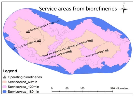
Figure 4.
The service area of existing biorefineries within specific travel times.
However, the coverage increased to 96.8% and 90.3% for an additional hour of driving time. Table 5 illustrates the size of service areas within 60 min, 120 min, and 180 min. Since we did not incorporate the cutoff costs at facilities such as loading/unloading time, the maximum travel time to collect biomass from a potential facility was approximately six hours.
Table 5.
Service area within different travel time blocks. Most suitable sites are shown to be between 1 and 2 h travel time to the biomass refineries.
3.3. Shortest Transportation Route
Figure 5 shows the shortest paths from the six biorefineries in Missouri to 116 potential sites in scenario 1 and 3343 potential sites in scenario 2, respectively. Based on the road system, the Closest-Facility apparatus determined the shortest path from each plant to each of the potential sites. Table 6 and Table 7 present the results of the suitable selection for scenarios 1 and 2, respectively, where each biorefinery is presented with its potential growing site (facility), area (in hectares), and potential yield (in Mg).
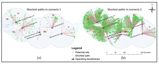
Figure 5.
The shortest path from existing biorefinery plants to potential switchgrass cultivation locations (a) in scenario 1 and (b) in scenario 2. The refineries are connected to their potential incidents, which would serve as sources of biomass.
Table 6.
Potential feedstock by biorefinery in scenario 1.
Table 7.
Potential feedstock by biorefinery in scenario 2.
In scenario 2, the Lifeline Foods LLC and ICM Pilot Int Cell plant are estimated to gather the largest amount of biomass among biorefineries since there are 1387 potential sites potentially accessible from them. The accumulated area of these sites accounts for 51% of the total potential area. Following this plan are Golden Triangle Energy LLC and Poet Biorefining 2, which can access 755 and 605 sites, respectively.
3.4. Least Transportation Costs
Using the shortest path result (Figure 5) and estimated regional transport cost per minute of travel, we estimated the transportation cost for collecting switchgrass as their feedstock. The cost in scenario 1 ranged from $3.62–$23.12 (Mg−1), and $4.0–$22.52 (Mg−1) in scenario 2. The wide range of transportation costs was caused by a broad range of distances carried by potential haul trucks. These distances were very dependent on the spatial distributions of potential sites. However, using a Monte Carlo simulation for 10,000 repetitions showed that 90% of transportation costs fell in the range of $3.70–$14.75 per Mg in scenario 1 and $2.75–$14.66 per Mg in scenario 2.
Further analysis of scenario 2 results showed that the least cost biorefinery point was Show Me Ethanol (3); this biorefinery also covered 6% of the potential switchgrass (see Figure 6). While it had the lowest transport cost, it covers very little of the study area effectively. Conversely, LF, LLC & ICM Pilot Int. Cell (2) covered 51% of the area while having the second-lowest transport cost. This makes it a prime candidate as a potential pilot plant for the region, with both low transportation costs and ideal land quality.
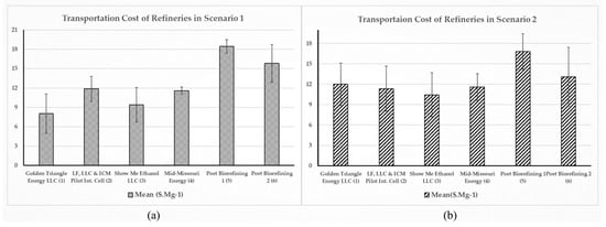
Figure 6.
Transportation cost of refineries in scenarios. (a) in scenario 1, (b) in scenario 2.
Figure 7 shows a histogram of the probability density of transportation cost based on the shortest paths in scenario 1 and scenario 2. The difference in transportation costs between the scenarios illustrates the influence of land use land cover to the end cost. The results indicate that marginal lands are not located proximally to the existing refineries.
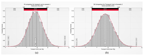
Figure 7.
Transportation cost mean by refineries. (a) in scenarios 1, (b) in scenario 2.
3.5. Ecosystem Services
Broader impacts of these shifts are captured by ecosystem benefits given by land-use change to switchgrass. Namely, the InVEST models for Carbon Storage, Annual Water Yield, and Sediment Delivery Ratio were employed to quantify the feedback on carbon stocks, total water yield, surface erosion, and local streamflow caused by land-use conversion to switchgrass. Table 8 demonstrates changes in ecosystem services in each scenario in terms of carbon storage, water yield, sediment total, and sediment export. Table 8 also shows the results of scenarios 1 and 2 compared to the base case represented by the rate of change. Shifting to switchgrass showed a generally positive impact on both scenarios for the ecosystem. Although there was a small 0.004%, reduction in annual water yield in scenario 1, scenario 2 showed a strong positive effect on water yield. The effect is similar across the board, as scenario 1 simply identified too little available land for switchgrass growth for a substantial regional impact. However, scenario 2 identified far more available land, which, when cultivated, had a much more significant impact on ecosystem function.
Table 8.
Potential ecosystem services feedback from suggested land use land cover change.
Carbon stocks could be increased by up to 3.325%, equivalent to 59,281,2967 Mg, by switching marginal land and non-food cropland to switchgrass due to the deep root system of switchgrass [51]. Soil erosion would decline substantially, with a reduction of about 2.14% in total sediment and a 5.06% decline in sediment export. Additionally, around 34.4 million m3 of water would be allowed to infiltrate into the soil layer or drain to the stream network and account for a 1.36% increase in available water yield compared to the base case.
Subsidies have often been proposed for switchgrass cultivation [4,9], and ecosystem service benefits can be used to help justify these subsidies beyond end-use carbon offsets. Carbon stocks alone increase between 33.14–72.54 Mg per hectare for the land cover types studied. This increases the value of growing switchgrass as a crop over its utility as a bioenergy feedstock, which can be used as a reason for additional subsidies based on an agreed carbon price divided out by years of cultivation.
4. Discussion
Expanding bioenergy feedstock supply while avoiding competition with food crops is a priority. This research estimates the potential for energy crop cultivation by considering consequences of land-use change and accounting for a range of ecosystem benefits. We used the combination of fuzzy logic and network optimization to evaluate potential switchgrass-based biomass supply and applied the InVEST ecosystem service approach to validate our selection for land cover transitions in Missouri. Furthermore, we count for the variations in yield, operation costs during growing and transporting biomass from potential sites to existing biorefineries within the study area.
Our results show that this methodology can be used to find the biorefineries with the highest potential for new feedstocks. In the case study, Show Me Ethanol LLC was the most efficient refinery in terms of biomass transport (see Table 6 and Table 7). However, Lifeline Foods, LLC & ICM Pilot Int. Cell can potentially benefit from the highest land availability. Given that this plant is already collecting cellulosic materials to produce biofuel, it may be suitable to consider switchgrass-based biofuel production at this facility.
Switchgrass cultivation in Missouri shows some promise given the requisite infrastructure and demand. However, in scenario 1, where switchgrass cultivation was considered only on marginal land, we found that the potential regions could only cover about 4755 ha. The area of potential regions could increase to 1,766,454 ha in scenario 2, where non-food cropland such as grasslands, alfalfa, and pasture/hay were considered. The potential regions were spread mostly through the northwestern and the western regions of the research area; the unequal distribution can be explained by several factors, including the steep slope of the terrain and critical species’ habitats in the southern and the southeastern sections of the study area preventing development. In scenario 2, using suitable regions to grow switchgrass could yield around 18 × 106 ÷ 39.6 × 10⁶ Mg of biomass. As the 2016 Billion-Ton Report, 56 gal ton−1 (approximately 225.325 L Mg−1) can be used as the conversion rate for the transformation of biomass to biofuel [9]. Using this assumption, the biorefineries could produce about 4055 × 106 ÷ 8923 × 106 L of bioethanol depending on the level of fertilization and cultivation of the switchgrass (see Table 2 and Table 3). Given the relatively small study area and the clustered nature of suitable land, the conversion plan in scenario 2 could be a potential approach to achieve large-scale production of bioenergy.
The ecosystem services provided by such an endeavor provide substantial benefit, including directly providing 59 million tons of carbon capture in addition to the carbon offset from ethanol use. The decrease in sedimentation and increased available water in a heavily agricultural area is significant as well.
The InVEST models applied in this research revealed the significant benefit switchgrass could have on ecosystem services, including annual water yield, carbon storage, and soil erosion. The outputs confirmed that converting suitable areas from original crops to switchgrass could yield positive feedback to the environment. In scenario 1, the impacts were indistinct because the land cover change is too small, less than 1% of the total area. In scenario 2, in contrast, the impacts on all studied services were sustainably remarkable. Besides yielding remarkable biomass, switchgrass is well-known for its ability to reduce soil erosion, increase soil organic carbon, and increase carbon sequestration [15]. In scenario 2, where almost 14% of the total area is employed growing switchgrass, we see a 3.33% increase in carbon storage, which accounts for around 59.3 × 10⁶ Mg of carbon.
Similarly, alternative land-use can generate 0.28 Mg ha−1 less sedimentation than idle cropland and fallow land. Also, while no habitat risk assessment was conducted, there are studies on the benefit of growing switchgrass to species across the US [26]. For example, Werling et al. confirmed that low-input cultivation switchgrass enhances biodiversity in a study conducted in Michigan and Wisconsin [23]. Other studies, e.g., Bies and Hartman and Werling suggested that switchgrass provides multiple ecological niches for different species, including birds, insects, reptiles, and mammals by maintaining multi-dimension habitat structure [23,61,62]. The lack of adequate field tests for our region prevented analyzing the positive and negative externalities of biodiversity and increased fertilization on switchgrass cultivation.
While the extent of this research goes beyond what many have previously accomplished [12], that the study does not use yield as a normalizing factor for transportation cost, as costs are assumed to be incurred by optimized, fully loaded trucks. Additionally, transportation in our case only includes trucks as a potential vehicle of transport, as there is no existing infrastructure for other transportation vectors for most existing biorefineries in the study area. We also feel that analysis can be improved by using partial values in fuzzy logic rather than using a discrete, strict yes/no terminology. Furthermore, a full implementation might require additional considerations for the interactions between the various conditions that affect switchgrass growth, particularly the interplay between rainfall, soil type, and yield, where higher precipitation in conjunction with well-drained soils might produce favorable conditions [46]. Given the seasonal nature of the temperature data required for this study, we used recorded station data from the study region. Finally, as we only considered potentially expanding existing biorefineries for switchgrass-based biofuels, as opposed to building a new plant, our analysis can be extended by identifying the most suitable locations for cellulosic biorefineries.
5. Conclusions
Our study shows that existing biorefineries can relatively quickly increase their access to cellulosic feedstocks, focusing on using marginal land and non-food cropland to build towards greater bioenergy use ultimately. The analysis evaluated the accessibility of potential bioenergy based on locating suitable areas in which biomass can be produced and minimizing the transport cost from existing biorefineries to their potential suppliers. It identified potential biomass suitability zones based on favorable conditions as well as possible constraints such as developed urban areas, biodiversity, ecosystem services, and traditional food crop zones. Then, based on these cultivation zones, the study evaluated accessibility based on potential bioenergy crop yield and the least cost of transportation of locally existing biorefineries. This study can be used to provide data for developing a biomass supply system capable of operating cost-effectively at a commercial scale [9]. Based on the location of the biomass suitability zones, biorefineries can also consider partnering with local farmer associations or entering into contracts with farmers to ensure year-round biomass supply.
We used the methodology to assess the suitability of switchgrass-based bioenergy in Missouri and neighboring states as a case study. The case study results suggest that while that degraded or marginal land has been considered as a resource for growing switchgrass as an energy crop, the potential yield harvested from marginal land alone is not enough for proper development of the bioethanol industry in the state of Missouri. While switchgrass might not be the ideal crop in all non-food croplands, utilizing grasslands and pasture/hay lands for switchgrass cultivation might contribute significantly towards cellulosic-based biofuel expansion. Our results show new information for determining where this kind of analysis can be deployed and what biorefineries may be optimal by considering feedstock, transportation, and associated cost constraints. By following this method, one may find potential biorefinery locations in their research, which will lead to increased efficiency in feedstock transportation.
While our model addresses many factors that play a major role in the potential development of cellulosic-based biofuel production, future research should continue to expand on external factors to provide more details to inform effective decision-making. Our model focuses primarily on positive ecosystem services associated with bioenergy development, which could be expanded on to address the complex extensive feedback systems that industry development has on the environment. For example, the effects of monoculture expansion have been associated with adverse environmental consequences which alter the natural ecosystem even in systems utilizing native species [63]. Challenges associated with monoculture, such as reduced pollination and soil microbe biodiversity, should be explored for switchgrass development. Future work can incorporate additional transportation networks, ecosystem service externalities, and partial values in fuzzy analysis and variable interactions to add to the body of knowledge in this area and contribute towards policy planning, economic feasibility modeling, and best practices development and deployment.
Supplementary Materials
The following are available online at https://www.mdpi.com/1996-1073/13/17/4516/s1, Table S1: InVEST parameter values for the sediment delivery ratio (SDR) mode: biophysical table. Column headings follow naming conventions in Sharp et al. (2016), Table S2: InVEST parameter values for the annual water yield model: biophysical table. Column headings follow naming conventions in Sharp et al. (2016), Table S3: InVEST parameter values for the carbon storage model: biophysical carbon table. Column headings follow naming conventions in Sharp et al. (2016), Table S4: Spatial data sources used in the InVEST models.
Author Contributions
Conceptualization, H.T.G.N., E.L., P.L. and P.B.; Data curation, H.T.G.N. and E.L.; Formal analysis, H.T.G.N., E.L., P.L. and T.W.; Funding acquisition, P.L.; Investigation, E.L. and P.L.; Methodology, H.T.G.N., E.L., P.L. and P.B.; Project administration, P.L.; Resources, P.L.; Software, H.T.G.N. and E.L.; Supervision, H.T.G.N., E.L. and P.L.; Validation, H.T.G.N., E.L. and P.L.; Visualization, H.T.G.N. and E.L.; Writing—original draft, H.T.G.N., E.L. and P.B.; Writing—review & editing, P.L., T.W. and P.B. All authors have read and agreed to the published version of the manuscript.
Funding
This research was funded by the National Science Foundation Award 1555123 and the U.S. Department of Agriculture National Institute of Food and Agriculture Grant 2012-67009-19742.
Acknowledgments
Any opinion, findings, conclusions, or recommendations expressed in this material are those of the authors and do not reflect the views of the Montclair State University, National Science Foundation, U.S. Department of Agriculture, U.S. Department of Energy Bioenergy Technologies Office (BETO) or the Idaho National Laboratory.
Conflicts of Interest
The authors declare no conflict of interest.
References
- Hiloidhari, M.; Baruah, D.; Singh, A.; Kataki, S.; Medhi, K.; Kumari, S.; Ramachandra, T.V.; Jenkins, B.M.; Thakur, I.S. Emerging role of Geographical Information System (GIS), Life Cycle Assessment (LCA) and spatial LCA (GIS-LCA) in sustainable bioenergy planning. Bioresour. Technol. 2017, 242, 218–226. [Google Scholar] [CrossRef]
- Tilman, D.; Socolow, R.; Foley, J.A.; Hill, J.D.; Larson, E.; Lynd, L.R.; Pacala, S.; Reilly, J.; Searchinger, T.; Somerville, C.; et al. Beneficial biofuels—The food, energy, and environment trilemma. Science 2009, 325, 270–271. [Google Scholar] [CrossRef] [PubMed]
- Fargione, J.; Hill, J.; Tillman, D.; Polasky, S.; Hawthorne, P. Land clearing and the biofuel carbon debt. Science 2008, 319, 1235–1238. [Google Scholar] [CrossRef] [PubMed]
- Burli, P.; Forgoston, E.; Lal, P.; Billings, L.; Wolde, B. Adoption of switchgrass cultivation for biofuel under uncertainty: A discrete-time modeling approach. Biomass Bioenergy 2017, 105, 107–115. [Google Scholar] [CrossRef]
- Richard, T.L. Challenges in Scaling Up Biofuels Infrastructure. Science 2010, 329, 793–796. [Google Scholar] [CrossRef]
- Van Der Weijde, T.; Kamei, C.L.A.; Torres, A.F.; Vermerris, W.; Dolstra, O.; Visser, R.G.; Trindade, L.M. The potential of C4 grasses for cellulosic biofuel production. Front. Plant Sci. 2013, 4. [Google Scholar] [CrossRef]
- Luo, Y.; Miller, S. A game theory analysis of market incentives for US switchgrass ethanol. Ecol. Econ. 2013, 93, 42–56. [Google Scholar] [CrossRef]
- Schnepf, R. Cellulosic Ethanol: Feedstocks, Conversion Technologies, Economics, and Policy Options, Congressional Research Service, CRS R41460. October 2010. Available online: www.crs.gov (accessed on 10 April 2019).
- Langholtz, M.H.; Stokes, B.J.; Eaton, L. 2016 Billion-Ton Report: Advancing Domestic Resources for a Thriving Bioeconomy, Volume 1: Economic Availability of Feedstocks; US Department of Energy: Washington, DC, USA, 2016; p. 448.
- EPA. Final Renewable Fuel Standards for 2020, and the Biomass-Based Diesel Volume for 2021; EPA. December 2019. Available online: https://www.epa.gov/renewable-fuel-standard-program/final-renewable-fuel-standards-2020-and-biomass-based-diesel-volume#additional-resources (accessed on 18 August 2020).
- Voivontas, D.; Assimacopoulos, D.; Koukios, G.E. Assessment of biomass potential for power production: A GIS based method. Fuel Energy Abstr. 2002, 43, 118. [Google Scholar] [CrossRef]
- Beccali, M.; Columba, P.; D’Alberti, V.; Franzitta, V. Assessment of bioenergy potential in Sicily: A GIS-based support methodology. Biomass Bioenergy 2009, 33, 79–87. [Google Scholar] [CrossRef]
- Höhn, J.; Lehtonen, E.; Rasi, S.; Rintala, J. A Geographical Information System (GIS) based methodology for determination of potential biomasses and sites for biogas plants in southern Finland. Appl. Energy 2014, 113, 1–10. [Google Scholar] [CrossRef]
- Sultana, A.; Kumar, A. Optimal siting and size of bioenergy facilities using geographic information system. Appl. Energy 2012, 94, 192–201. [Google Scholar] [CrossRef]
- ESRI. ArcGIS Help 10.1. ArcGIS Resources. Available online: http://resources.arcgis.com/en/help/main/10.1/index.html#/Location_allocation_analysis/004700000050000000/ (accessed on 2 November 2018).
- Hartman, J.C.; Nippert, J.B.; Springer, C.J. Ecotypic responses of switchgrass to altered precipitation. Funct. Plant Biol. 2012, 39, 126. [Google Scholar] [CrossRef] [PubMed]
- Mitchell, R.; Vogel, K.P.; Sarath, G. Managing and Enhancing Switchgrass as a Bioenergy Feedstock. 2008, p. 11. Available online: https://doi.org/10.1002/bbb.106 (accessed on 20 June 2020).
- Gallagher, E. The Gallagher Review of the Indirect Effects of Biofuels Production. Renewable Fuels Agency (RFA). July 2008. Available online: https://www.unido.org/sites/default/files/2009-11/Gallagher_Report_0.pdf (accessed on 20 September 2019).
- Lewis, S.; Kelly, M. Mapping the Potential for Biofuel Production on Marginal Lands: Differences in Definitions, Data and Models across Scales. ISPRS Int. J. Geo-Inf. 2014, 3, 430–459. [Google Scholar] [CrossRef]
- Kraxner, F.; Aoki, K.; Kindermann, G.; LeDuc, S.; Albrecht, F.; Liu, J.; Yamagata, Y. Bioenergy and the city—What can urban forests contribute. Appl. Energy 2016, 165, 990–1003. [Google Scholar] [CrossRef]
- Saha, M.; Eckelman, M.J. Geospatial assessment of regional scale bioenergy production potential on marginal and degraded land. Resour. Conserv. Recycl. 2018, 128, 90–97. [Google Scholar] [CrossRef]
- Zhao, X.; Monnell, J.D.; Niblick, B.; Rovensky, C.D.; Landis, A.E. The viability of biofuel production on urban marginal land: An analysis of metal contaminants and energy balance for Pittsburgh’s Sunflower Gardens. Landsc. Urban Plan. 2014, 124, 22–33. [Google Scholar] [CrossRef]
- Hartman, J.C.; Nippert, J.B. Physiological and growth responses of switchgrass (Panicum virgatum L.) in native stands under passive air temperature manipulation. GCB Bioenergy 2013, 5, 683–692. [Google Scholar] [CrossRef]
- Dijkstra, E.W. A Note on Two Problems in Connexion with Graphs. Numer. Math. 1959, 1, 269–271. [Google Scholar] [CrossRef]
- Polasky, S.; Nelson, E.; Pennington, D.; Johnson, K.A. The Impact of Land-Use Change on Ecosystem Services, Biodiversity and Returns to Landowners: A Case Study in the State of Minnesota. Environ. Resour. Econ. 2011, 48, 219–242. [Google Scholar] [CrossRef]
- Fike, J.H.; Pease, J.W.; Owens, V.; Farris, R.L.; Hansen, J.L.; Heaton, E.A.; Hong, C.O.; Mayton, H.S.; Mitchell, R.B.; Viands, D.R. Switchgrass nitrogen response and estimated production costs on diverse sites. GCB Bioenergy 2017, 9, 1526–1542. [Google Scholar] [CrossRef]
- Boyer, C.N.; Roberts, R.K.; English, B.C.; Tyler, D.D.; Larson, J.A.; Mooney, D.F. Effects of soil type and landscape on yield and profit maximizing nitrogen rates for switchgrass production. Biomass Bioenergy 2013, 48, 33–42. [Google Scholar] [CrossRef]
- Hui, D.; Yu, C.-L.; Deng, Q.; Dzantor, E.K.; Zhou, S.; Dennis, S.; Sauvé, R.; Johnson, T.L.; Fay, P.A.; Shen, W.; et al. Effects of precipitation changes on switchgrass photosynthesis, growth, and biomass: A mesocosm experiment. PLoS ONE 2018, 13, e0192555. [Google Scholar] [CrossRef] [PubMed]
- Ethanolproducer. Ethanol Producer Magazine. 29 June 2018. Available online: http://ethanolproducer.com/plants/listplants/US/Operational/All/page:1/sort:state/direction:asc (accessed on 10 April 2018).
- DOE’s. Biorefinery Optimization Workshop Summary Report; Workshop Summary; U.S. Department of Energy: Chicago, IL, USA, 2016. Available online: https://www.energy.gov/sites/prod/files/2017/02/f34/biorefinery_optimization_workshop_summary_report.pdf (accessed on 20 June 2020).
- Analysis Division and FMCSA. 2010–2011 Hours of Service Rule Regulatory Impact Analysis RIN 2126-AB26; U.S. Department of Transportation—Federal Motor Carrier Safety Administration: Washington, DC, USA, December 2011.
- Arguez, A.; Durre, I.; Applequist, S.; Squires, M.; Vose, R.; Yin, X.; Bilotta, R. NOAA’s U.S. Climate Normals (1981–2010); NOAA National Centers for Environmental Information: Boulder, CO, USA, 2010. [CrossRef]
- Homer, C.; Dewitz, J.; Yang, L.; Jin, S.; Danielson, P.; Xian, G.; Coulston, J.; Herold, N.; Wickham, J.; Megown, K. Completion of the 2011 National Land Cover Database for the conterminous United States-Representing a decade of land cover change information. Photogramm. Eng. Remote Sens. 2015, 81, 345–354. [Google Scholar]
- ESRI. USA Street Map. ArcGIS. 22 May 2010. Available online: https://www.arcgis.com/home/item.html?id=f28762ef94ef4700864fd57d0ef7ec7a (accessed on 28 March 2018).
- USDA/NRCS—National Geospatial Center of Excellence. National Elevation Data 30 Meter. Present 2000. Available online: http://ned.usgs.gov/ (accessed on 21 November 2017).
- Soil Survey Staff. Web Soil Survey; Natural Resources Conservation Service, United States Department of Agriculture; Washington, DC, USA. Available online: https://datagateway.nrcs.usda.gov/GDGOrder.aspx (accessed on 21 November 2017).
- Perdue, J.H. The Biomass Site Assessment Tool (BioSAT) Final Report; USDA Forest Service, Southern Research Station: Asheville, NC, USA, May 2011. Available online: http://www.biosat.net/Pdf/The_Biomass_Site_Assessment_Tool.pdf (accessed on 27 June 2020).
- Jungers, J.M.; Sheaffer, C.C.; Lamb, J.A. The Effect of Nitrogen, Phosphorus, and Potassium Fertilizers on Prairie Biomass Yield, Ethanol Yield, and Nutrient Harvest. BioEnergy Res. 2015, 8, 279–291. [Google Scholar] [CrossRef]
- Lawrence, J.; Cherney, J.; Barney, P.; Ketterings, Q. Establishment and Management of Switchgrass; Series 20; Cornell University Cooperative Extension: New York, NY, USA, 2006; Available online: http://forages.org/files/bioenergy/Switchgrassfactsheet20.pdf (accessed on 22 June 2020).
- Kim, S.; Williams, A.; Kiniry, J.R.; Hawkes, C.V. Simulating diverse native C4 perennial grasses with varying rainfall. J. Arid Environ. 2016, 134, 97–103. [Google Scholar] [CrossRef]
- Sherrard, M.E.; Joers, L.C.; Carr, C.M.; Cambardella, C.A. Soil type and species diversity influence selection on physiology in Panicum virgatum. Evol. Ecol. 2015, 29, 679–702. [Google Scholar] [CrossRef]
- Grumbach, S. Handling Interpolated Data. Comput. J. 2003, 46, 664–679. [Google Scholar] [CrossRef]
- U.S Fish & Wildlife Service. U.S. FWS Threatened & Endangered Species Active Critical Habitat Report. ECOS Environmental Conservation Online System Conserving the Nature of America. 22 June 2018. Available online: https://ecos.fws.gov/ecp/report/table/critical-habitat.html (accessed on 29 June 2018).
- Li, Y.-F.; Wang, Y.; Tang, Y.; Kakani, V.; Mahalingam, R. Transcriptome analysis of heat stress response in switchgrass (Panicum virgatum L.). BMC Plant Biol. 2013, 13, 153. [Google Scholar] [CrossRef]
- Sanderson, M.; Reed, R.; Ocumpaugh, W.; Hussey, M.; Van Esbroeck, G.; Read, J.; Tischler, C.; Hons, F. Switchgrass cultivars and germplasm for biomass feedstock production in Texas. Bioresour. Technol. 1999, 67, 209–219. [Google Scholar] [CrossRef]
- Baskaran, L.; Jager, H.I.; Schweizer, P.E.; Srinivasan, R. Progress toward Evaluating the Sustainability of Switchgrass as a Bioenergy Crop using the SWAT Model. Trans. ASABE 2010, 53, 1547–1556. [Google Scholar] [CrossRef]
- Kiniry, J.R.; Schmer, M.R.; Vogel, K.P.; Mitchell, R.B. Switchgrass Biomass Simulation at Diverse Sites in the Northern Great Plains of the U.S. BioEnergy Res. 2008, 1, 259–264. [Google Scholar] [CrossRef]
- Smith, R. Switchgrass Production Offers Opportunities, Growing Challenges; Southwest Farm Press: 6 December 2007. Available online: https://www.farmprogress.com/switchgrass-production-offers-opportunities-growing-challenges (accessed on 27 June 2020).
- Thomas, M.A.; Ahiablame, L.M.; Engel, B.A.; Chaubey, I. Modeling Water Quality Impacts of Growing Corn, Switchgrass, and Miscanthus on Marginal Soils. J. Water Resour. Prot. 2014, 6, 1352–1368. [Google Scholar] [CrossRef]
- Jager, H.I.; Baskaran, L.M.; Brandt, C.C.; Davis, E.B.; Gunderson, C.A.; Wullschleger, S.D. Empirical geographic modeling of switchgrass yields in the United States. GCB Bioenergy 2010, 2, 248–257. [Google Scholar] [CrossRef]
- Garland, C.; Bates, G.; Clark, C.; Dalton, D. Growing and Harvesting Switchgrass for Ethanol Production in Tennessee; University of Tennessee Extension: Knoxville, TN, USA, May 2008; Available online: https://trace.tennessee.edu/utk_agexbiof/6/ (accessed on 20 June 2020).
- Perlack, R.D.; Stokes, B.J. U.S. Billion-Ton Update: Biomass Supply for a Bioenergy and Bioproducts Industry; US Department of Energy: Washington, DC, USA, August 2011; p. 227.
- Casavant, K.; Denicoff, M.; Jessup, E.; Taylor, A.; Nibarger, D.; Sears, D.; Khachatryan, H.; McCracken, V.; Prater, M.; Bahizi, P. Study of Rural Transportation Issues; U.S. Department of Agriculture, Agricultural Marketing Service: Washington, DC, USA, April 2010. [CrossRef]
- Sharp, R.; Tallis, H.T.; Ricketts, T.; Guerry, A.D.; Wood, S.A.; Chaplin-Kramer, R.; Bierbower, W. InVEST +VERSION+ User’s Guide. The Natural Capital Project, Stanford University, University of Minnesota, The Nature Conservancy, and World Wildlife Fund; Stanford University: Stanford, CA, USA, 2016; Available online: http://data.naturalcapitalproject.org/nightly-build/invest-users-guide/html/index.html (accessed on 4 April 2020).
- Bagstad, K.J.; Ingram, J.C.; Lange, G.-M.; Masozera, M.; Ancona, Z.H.; Bana, M.; Kagabo, D.; Musana, B.; Nabahungu, N.L.; Rukundo, E.; et al. Towards ecosystem accounts for Rwanda: Tracking 25 years of change in flows and potential supply of ecosystem services. People Nat. 2019, 2, 163–188. [Google Scholar] [CrossRef]
- Murray, D.; Glidewell, S. An Analysis of the Operational Costs of Trucking; American Transportation Research Institute: Arlington, VA, USA, 2019; p. 48. [Google Scholar]
- Hooper, A.; Murray, D. An Analysis of the Operational Costs of Trucking; American Transportation Research Institute: Arlington, VA, USA, 2018; p. 49. [Google Scholar]
- AAA. Gas Prices. Available online: https://gasprices.aaa.com/?state=MO&fbclid=IwAR1x_10lK0B0_Thj06sNSkiRyuNakpkPmkmyl0KdjBXZvh_FzMl7Zpw3FqY (accessed on 20 June 2020).
- Jacobson, M.; Helsel, Z. NEWBio Switchgrass Budget for Biomass Production; PennState Cooperative Extension: University Park, PA, USA, April 2014; Available online: http://www.newbio.psu.edu/PublicationsFinal/SwitchgrassBudget.pdf (accessed on 25 June 2020).
- McGowan, A.R.; Min, D.-H.; Williams, J.R.; Rice, C.W. Impact of Nitrogen Application Rate on Switchgrass Yield, Production Costs, and Nitrous Oxide Emissions. J. Environ. Qual. 2018, 47, 228–237. [Google Scholar] [CrossRef] [PubMed]
- Bies, L. The Biofuels Explosion: Is Green Energy Good for Wildlife. Wildl. Soc. Bull. 2006, 34, 1203–1205. [Google Scholar] [CrossRef]
- Werling, B.P.; Dickson, T.L.; Isaacs, R.; Gaines, H.; Gratton, C.; Gross, K.L.; Liere, H.; Malmstrom, C.M.; Meehan, T.D.; Ruan, L.; et al. Perennial grasslands enhance biodiversity and multiple ecosystem services in bioenergy landscapes. Proc. Natl. Acad. Sci. USA 2014, 111, 1652–1657. [Google Scholar] [CrossRef]
- Timothy, L.D.; Katherine, L.G. Can the Results of Biodiversity-Ecosystem Productivity Studies Be Translated to Bioenergy Production? PLoS ONE 2015, 10, e0135253. [Google Scholar] [CrossRef]
© 2020 by the authors. Licensee MDPI, Basel, Switzerland. This article is an open access article distributed under the terms and conditions of the Creative Commons Attribution (CC BY) license (http://creativecommons.org/licenses/by/4.0/).