A Fast Method to Determine the Critical Depth of Cut for Various Rock Types

Abstract

Knowing correct values of the rock mechanical properties is crucial for many engineering applications in subsurface. Rocks may show two failure modes during cutting: ductile and brittle. In the ductile mode, rock deforms plastically, and the debris is powdered ahead of the cutting face. On the other hand, chips are the major cutting characteristics for the brittle failure during rock cutting. The critical depth of cut represents the transition point between these two models, so knowing this value helps better predict the failure mechanism of rock. In this paper, a new method is introduced based on measuring the roughness of the groove for determining the transition point of failure modes for every rock sample after the scratch test. The graph depicting the average change in the surface roughness ($R_t$) versus the scratched surface roughness ($\mathsf{\Delta }R$) can be used to identify the rock failure mode and determine the transition point for the cutting process. The value of this slope increases until the depth of cut reaches the transition point, and then the slope reaches a constant value. The main purpose of this paper is to estimate the critical depth of cut of different rock specimens employing the new surface roughness model.

1. Introduction

A grasp of the mechanical characteristics of various rocks for cutting and drilling is critical for different engineering applications such as tunneling and rock drilling. The primary concern in these applications is how the failure evolves in each particular condition. For instance, brittle failure mode is the desired cutting mechanism during drilling operations for achieving higher penetration rates [1]. In contrast, the ductile mode also known as strength driven mode is the preferred mechanism in concrete design as the deformation can be seen visually before an immediate collapse in the ductile mode [2]. Additionally, the size of the resultant drill cuttings impacts the hole cleaning efficiency in vertical wells, which consequently affects the rate of penetration [3]. The large size cuttings are difficult to transport through the horizontal section of the lateral wells and may settle down in the lateral section and form cuttings bed. Cutting beds are considered as one of the main reasons for the stuck pipe problems.

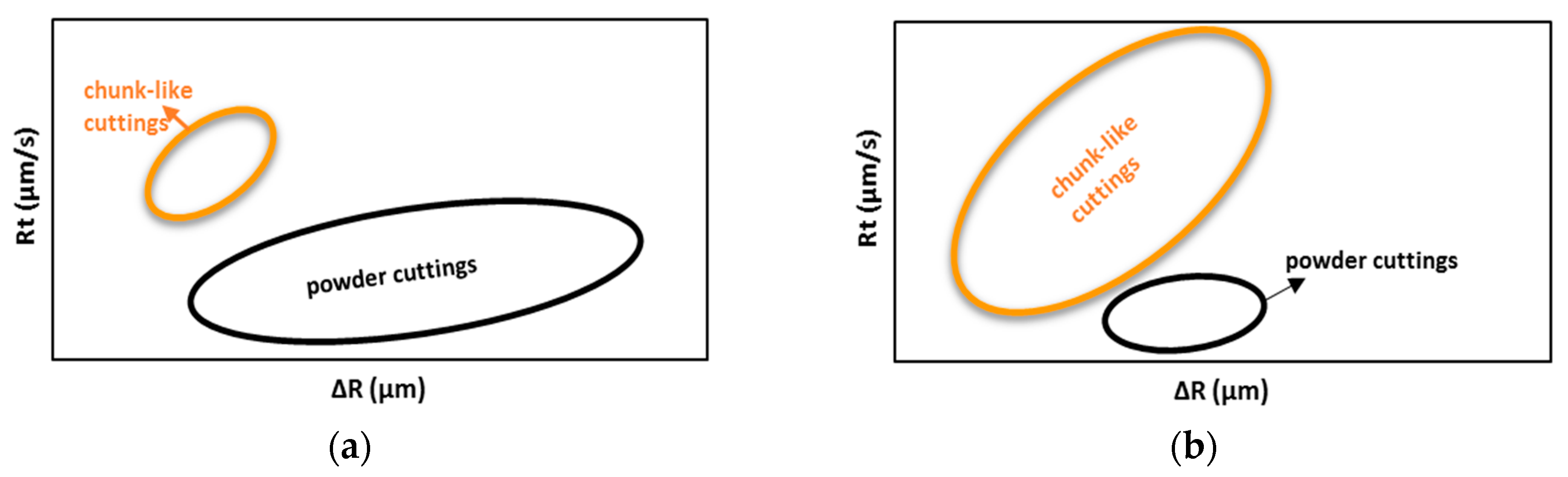
Two dominated failure mechanisms can be observed along the entire scratching action: ductile and brittle modes [4,5]. The ductile mode is the main failure mechanism when the depth of cut (DOC) is relatively small [6]. The rock acts as plastic in this situation and the cuttings are in the form of powder (see Figure 1a). As a result of grinding, the scratching process would become a smooth process with moderate fluctuations of the tangential force. On the other hand, the brittle mode reveals when the DOC reaches above the critical depth of cut (DOC). A discontinuous set of cracks is created underneath the cutter face in this model, as coalescence cracks propagate toward the free surface of the rock sample (see Figure 1b). During the chipping process, the cutting force starts to rise with the initiation of a crack. It has an upward trend until the crack propagation ends. Then, the shear force experiences a sharp drop, as cracks break into the groove surface [6].

The concept of the critical DOC was introduced when seeking the correct strength of industrial brittle materials such as glass and ceramics [7]. Molloy et al. [8] scratched the samples with a diamond cutter to obtain normal and tangential forces for different DOCs, they pointed out that chipping-type cutting occurs at deep DOCs. Additionally, Bifano and Fawcett [7] utilized the specific energy approach to investigate the relationship between rock features and critical DOC [7].

Later, Adachi et al. [9] developed the scratch test device in the current commercial form to find a correlation between the shear force during cutting and the unconfined compressive strength (UCS) of the rock [9]. This mechanical device scratches rock and metal samples using a single slanted PDC (Polycrystalline Diamond Compact) cutter. The scratch test has been used in various areas to obtain necessary engineering design information such as rock properties [10] or estimation of the cutting wear [11].

The scratch test device is kinematically controlled, which means that the cutting sweeps the sample surface at a constant velocity while the DOC is set to remain constant during the test. The shear and normal forces required to maintain this constant velocity are measured and recorded during the process. Detournay and Defourny [12] pointed out that there is a linear relationship between cutting force and DOC in the ductile mode (i.e., when the groove depth is shallow). In the case of the ductile mode, the shear (cutting) force can be expressed as:

$$F= ϵA,$$

(1)

where ϵ is the intrinsic specific energy, i.e., the amount of energy necessary to scratch a unit volume of rock. A represents the cross-sectional area of the rock surface touching the cutter. The cross-section area can be approximated for a sharp rectangular cutter as:

$$A=wd,$$

(2)

where w and d are the width of the cutter and the depth of the groove, respectively.

On the contrary, the linear relationship between $F_c$ and d turns into an upward slowing curve as the DOC increases. At this stage, this relationship follows Linear Elastic Fracture Mechanics (LEFM) and the ratio between the shear force and the groove depth can be written as:

$$F \propto K_{IC}w\sqrt{d},$$

(3)

where $K_{IC}$ is the fracture toughness of the rock. The validity of this equation has been proven numerically by Zhu et al. [13]. Shojaei and Dahi Taleghani [14] investigated this problem through continuum damage mechanics framework. Richard [5] claims that the correlation between the transition point for the rock failure mechanism and the intrinsic specific energy to be

$$d_c\propto {\left(\frac{K_{IC}}{ϵ}\right)}^2.$$

(4)

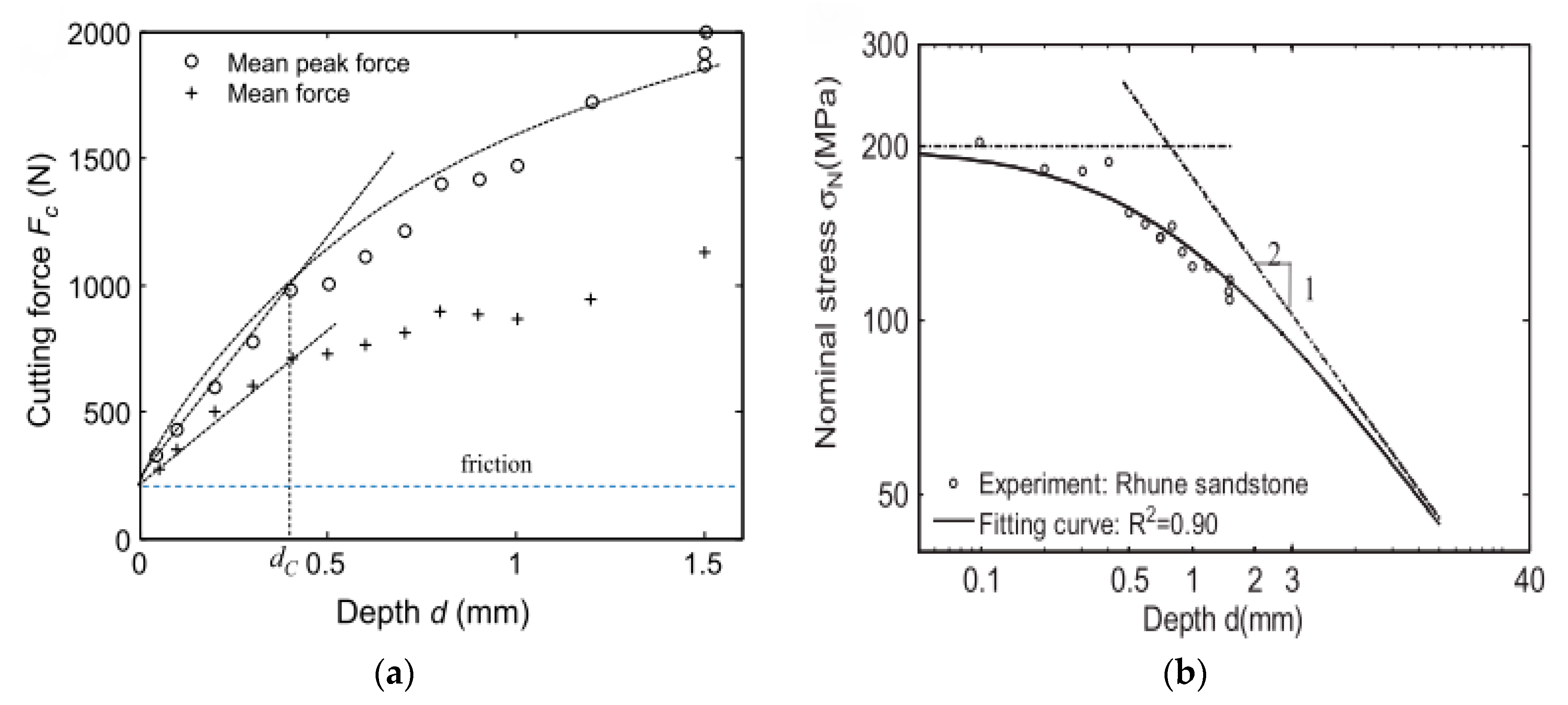
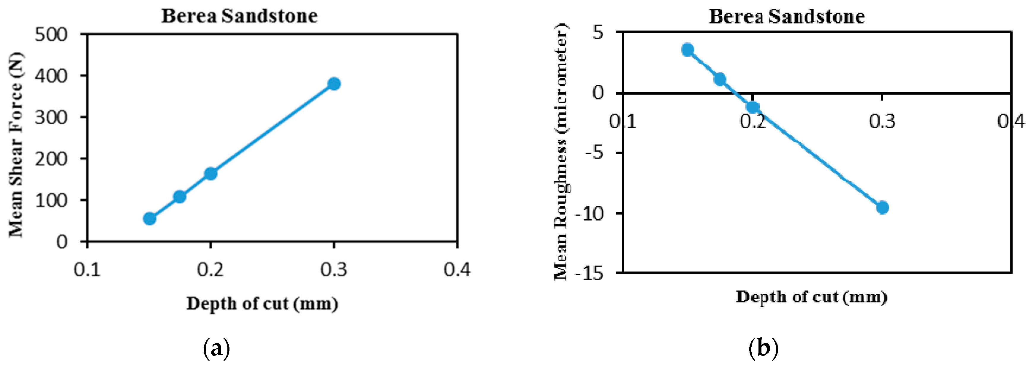
Nicodeme [4] did the scratch tests for three sandstone samples to obtain the averaged peak shear force and the mean cutting load evaluation with the rising DOC. These laboratory test results have proven that the averaged peak shear load increases linearly up to a point, presumed as the transition point between the ductile and brittle failure modes, such that the critical DOC is found at about 0.4 mm for Rhune sandstone (see Figure 2a).

Obtaining data from the ductile mode is critical for rock engineering purposes since these results are employed to find the uniaxial compressive strength value of rock specimens [10]. This situation persuaded researchers over the following years to conduct studies to delineate rock failure mechanisms and their implications. The size effect contribution has been formulated by Bazant et al. [15] for concrete, rock, and metal samples to explain the structure size effect over the failure transition point. The brittleness of material increases with increased structural volume and the nominal stress declines if the structure size goes above a critical point [16]. The nominal stress of cracked structures can be calculated as:

$${\sigma }_{Nu}=\frac{B{\sigma }_t}{\sqrt{1+D/D_0}},$$

(5)

where ${\sigma }_t$ is the tensile strength, $D$ represents structure volume. $D_0$ indicates the critical structure size.

Depending on $D$ and $D_0$ numbers, Equation (5) illustrates two characteristics of the size effect. For small values of $D$ (i.e., $D$ << $D_0$), the size effect can be ignored since ${\sigma }_{Nu}$ is almost constant. If the size of the material is very large ($D$ >> $D_0$), ${\sigma }_{Nu}$ has a relationship with the square root of the structure size and the inclination of bi-harmonic ${\sigma }_{Nu}$ verses $D$ plot is −1/2$\sqrt{D}$ [17]. If the structure is assumed as two-dimensional (2D), the nominal stress can be written as:

$${\sigma }_{Nu}= \frac{F}{bD},$$

(6)

where F shows the peak force value and $bD$ represents the structure cross-section. This formula can be used to calculate the nominal strength of undamaged structures, while Equation (5) is employed for a structure with serious damage.

In terms of the numerical modeling, some works have used the combination of Equations (5) and (6) to obtain the transition point of rock samples [18,19]. He et al. [19] employed the latter formula for shallow depths in their analysis assuming the cutting force has a linear correlation with DOC. On the other hand, the former formula is used for large DOCs to get a better fitting with the experimental results. The entire cutting process is defined as follows:

$${\sigma }_{Nu}=\{\begin{array}{cc}\hfill \frac{F}{bD},& d<D_0\hfill \\ \hfill \frac{B{\sigma }_t}{\sqrt{1+D/D_0}},& d>D_0\hfill \end{array} .$$

(7)

As seen from Equation (7), $D_0$ is the transition point between two different trends. In other words, $D_0$ illustrates the transition for the rock cutting process. Zhou and Lin [18] applied Equation (7) to Rhune sandstone sample to obtain acceptable fits. As highlighted in Figure 2b, this approach does not fit the Rhune sandstone results very well since the higher correlation coefficient value ($R^2)$ is 0.9. The critical DOC for Rhune sandstone is found by fitting cutting data to be 0.8 mm.

Another model for determining the transition point is proposed by He and Xu [20]. In their analysis, they used the specific cutting energy approach and found the critical DOC for limestone samples using the energy consumption difference between two failure modes. The specific cutting energy in the ductile mode for a sharp cutter can be calculated as:

$$E_d=\frac{F_c}{A}=\lambda ϵ,$$

(8)

where λ is a geometric factor related to the back-rake angle. As indicated in Equation (8), the specific cutting energy is not related to the DOC. The specific cutting energy remains constant even if the DOC increases in the strength driven mode; only the back-rake angle of the cutter increases the average cutting force [19].

On the other hand, chip-like cuttings in the brittle mode cause a much bigger damage volume than what is projected. Liu et al. [1] calculated the specific cutting energy in the brittle mode by finding the required cutting energy for removing a piece of rock given as:

$$E_b=k_b{d}^{-4/3}+k_p$$

(9)

where $k_b$ is related to the groove geometry and rock properties (such as Young’s modulus and fracture toughness), d represents DOC, and $k_p$ is a constant value. Equation (9) shows that the specific cutting energy declines with the groove depth in the brittle failure mode. The entire rock cutting process can be written in term of specific cutting energy:

$$E=\{\begin{array}{cc}\hfill \lambda ϵ,& d<d_c\hfill \\ \hfill k_b{d}^{-4/3}+k_p,& d>d_c\hfill \end{array},$$

(10)

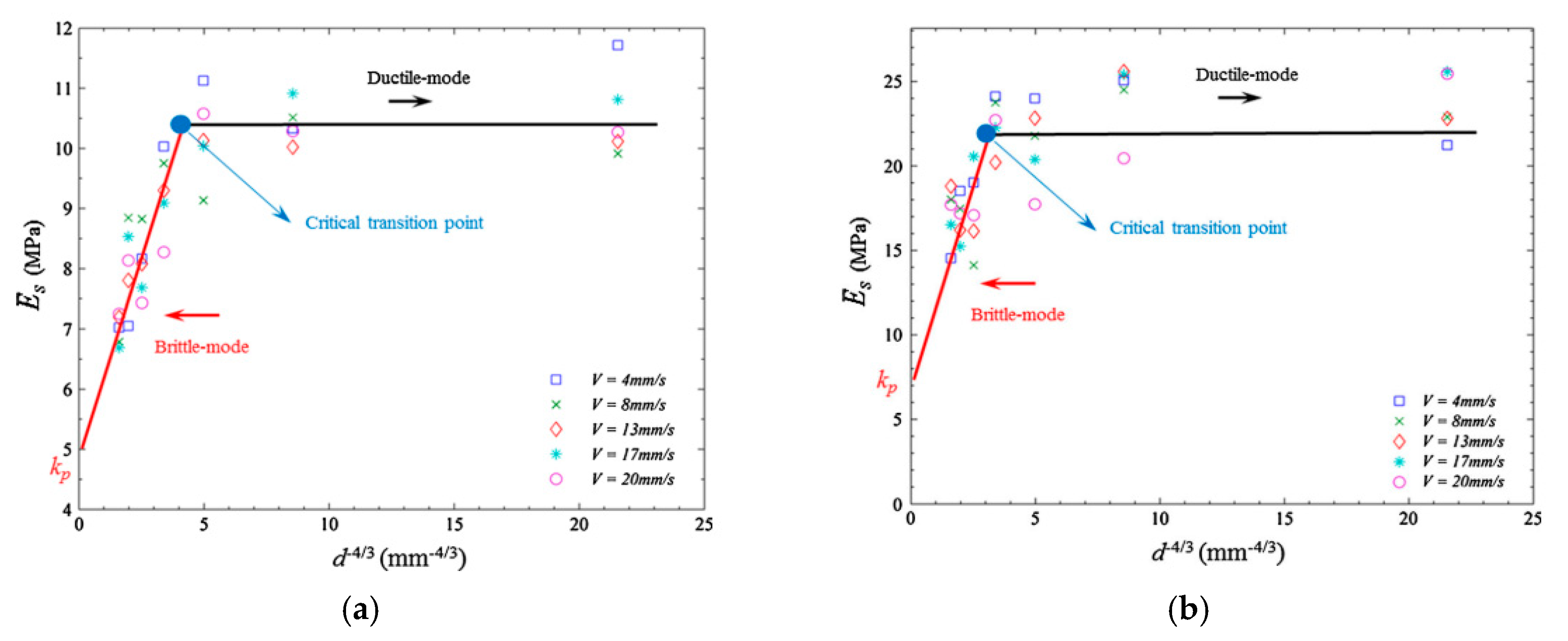
where $d_c$ illustrates the transition of rock cutting. Extensive laboratory experiments have been conducted by He et al. [19], Liu et al. [1], and He and Xu [20] to obtain the failure transition point of Tuffeau limestone and Savonnières limestone to validate the specific cutting energy approach. As illustrated in Figure 3, He and Xu [20] found the transition point of failure modes for two different limestone samples, respectively. However, this approach does not give accurate results when compared with experimental results and the highest number of the correlation coefficient ($R^2)$ is 0.82 in the fitting analysis.

Although these three methods (DD model, size effect method, and the specific energy approach) give approximate numbers for the transition point in different rocks, they all involve a curve fitting step. It is notable that some constants such as $k_b$ and $k_p$ are related to rock properties and back-rake angle so these numbers differ for each sample condition.

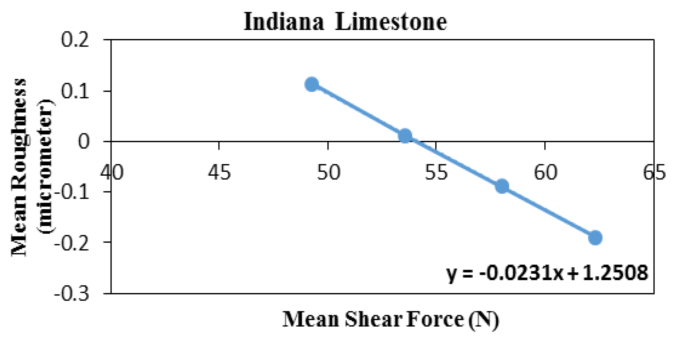
Despite numerous experimental and simulation studies that have been carried out to obtain information about the rock cutting process, the focus has been mainly on using cutter normal and shear forces [6,21]. Even though surface asperities can be measured with less complexity, there have not been any efforts to extract potential data that might be locked in the surface roughness to extract more information. The roughness is basically the difference between the scratched surfaces versus what is supposed to be in an ideal situation that rock is only scratched exactly at the given depth of cut. In the strength driven (ductile) mode, the cutter crushes a core sample to remove particles, so the surface of the groove remains smooth after the cutting process. On the other hand, chipping is a major rock breaking mechanism in the fracture driven (brittle) mode. Therefore, the surface of the cleared path is rough in this mode (see Figure 4).

This paper looks at the groove surface asperity and its relationship with critical DOC through a series of scratch tests conducted on samples of Berea sandstone, Indiana limestone, and Mudstone. The laboratory tests reveal the relationship between the shear force and the surface roughness during scratching. Moreover, the critical DOC is obtained using the groove roughness measured in these sedimentary rock samples. Lastly, the results of this work are expected to provide a more physical explanation for the ductile-brittle transition mechanism without difficulties involved in acquiring force data.

2. The Roughness Model

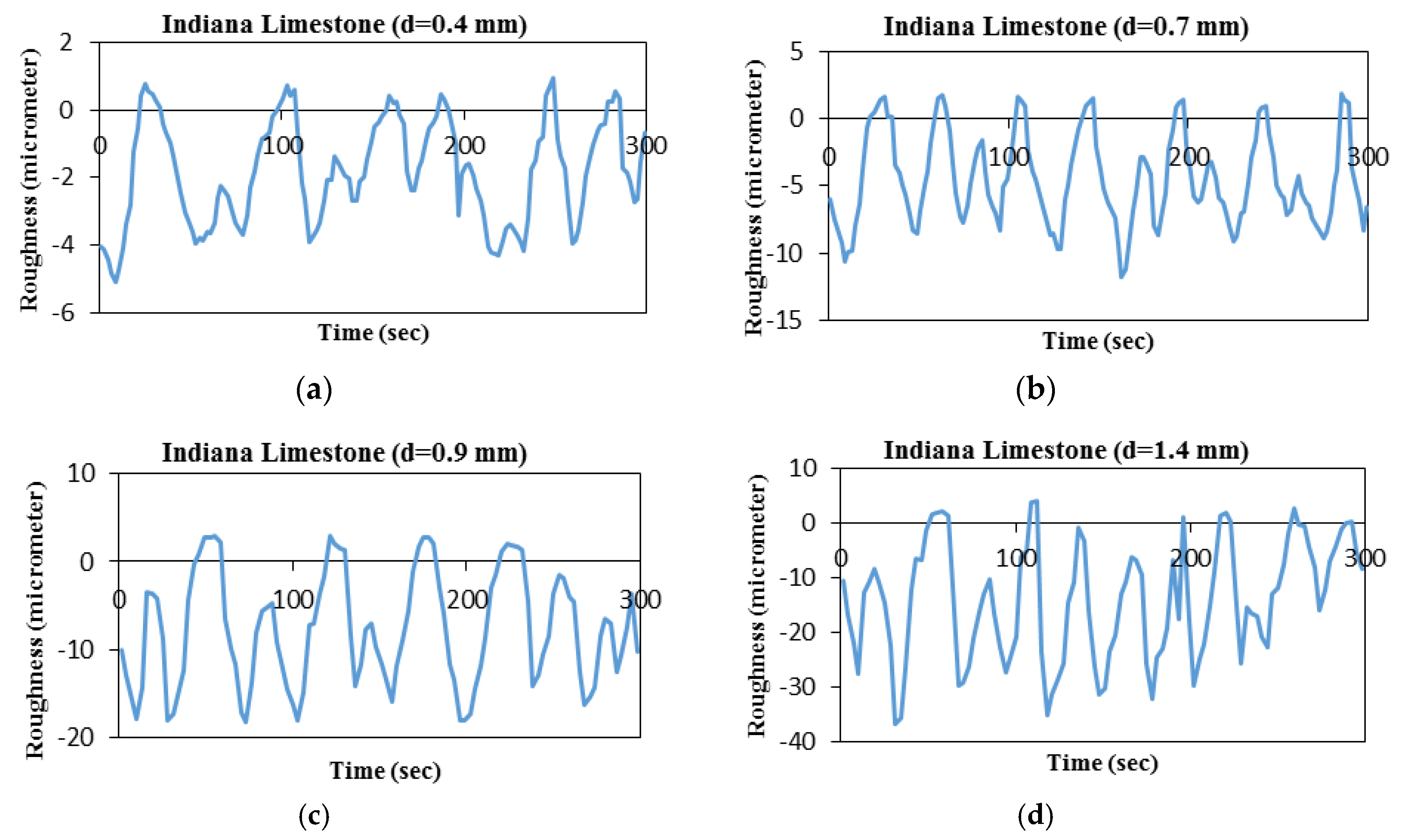
The ductile-brittle failure mode transition in the rock cutting process is an active research topic since it is a crucial issue for the cutter and bit design. The scratch test can be one of the known methods to identify this transitional feature. The observation of each scratch test shows that the rock surface after cutting is rough. The DOC is controlled and imposed by setting the cutter location during the cutting process but there are big height changes on the cleared surface path of rock specimens. Even though the surface roughness value is easily measured by an up-to-date scratch test device, the results have not been analyzed sufficiently to-date. It is notable that our study is basically limited to two-dimensional analysis although rock scratching might be considered as a 3D problem but by avoiding very narrow blades and boundary effects that might reveal along the blade edges, 2D analyses will provide more confidence in our analysis with less level of complexities of any 3D analysis.

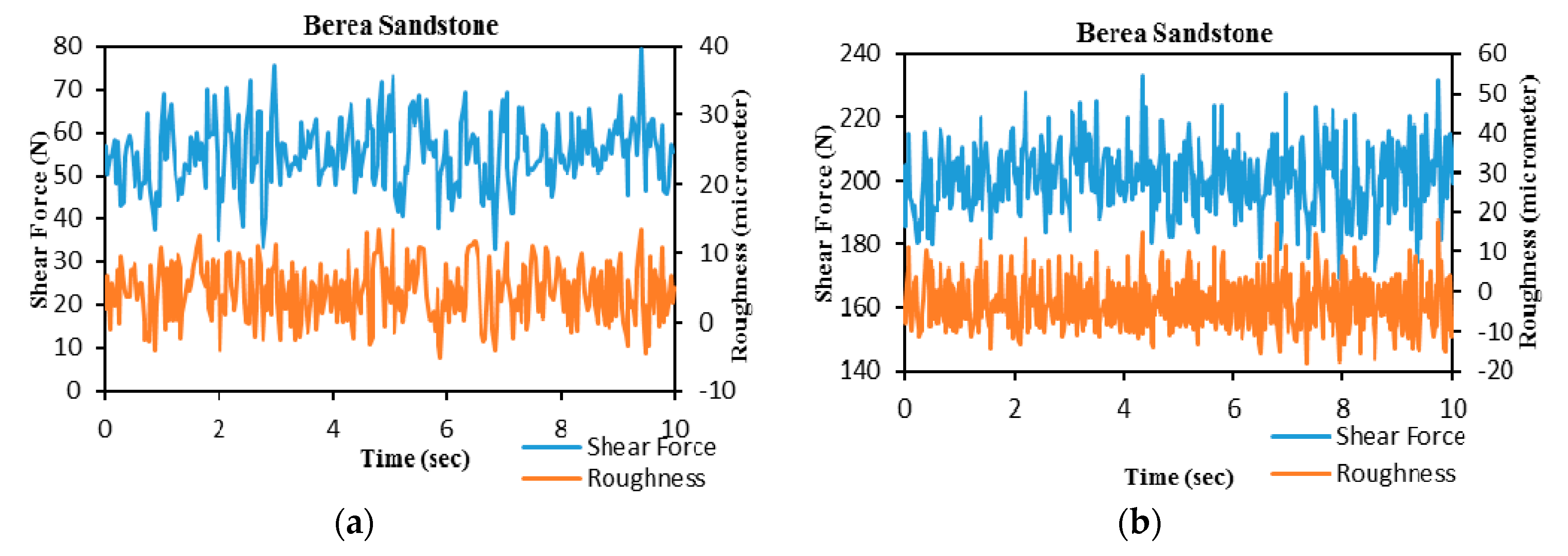
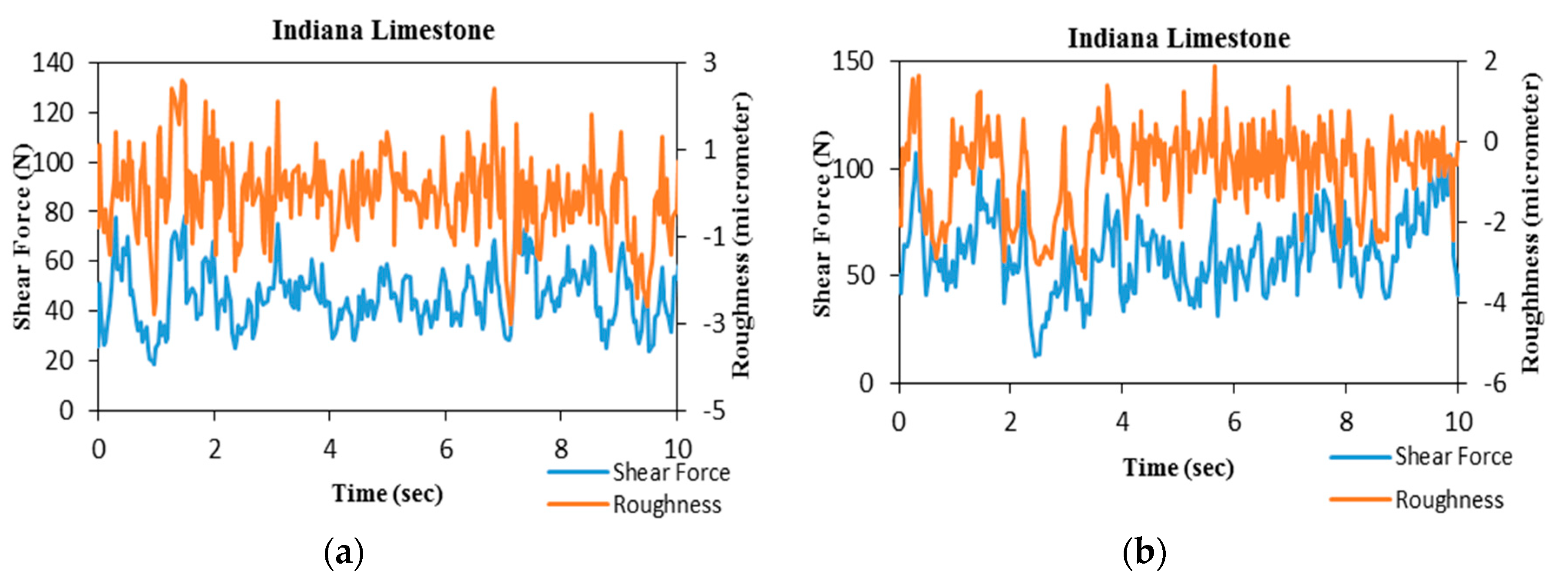
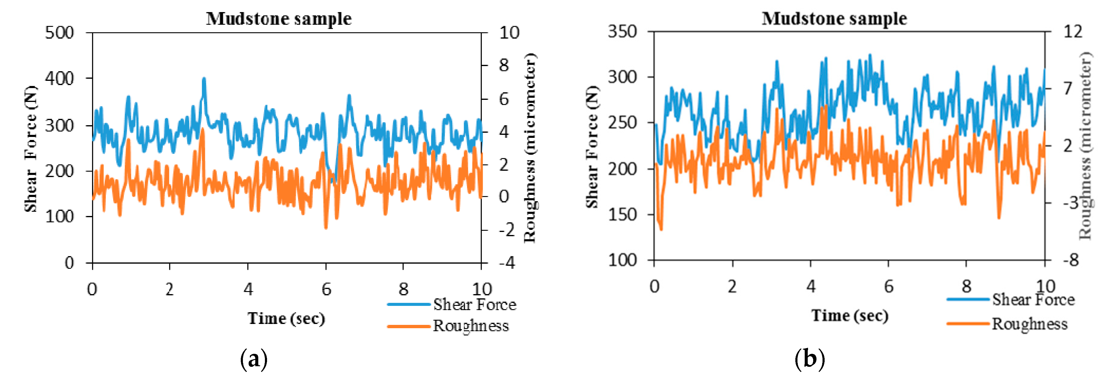
Scratch test results represent lines that show the rock cutting force and the surface roughness of rock follows a similar pattern during the entire cutting process (see Figure 5). In other words, the cutting groove surface is a reflection of the shear force variation, which is the nature of rock cutting. If the fluctuation of the tangential load is moderate, the resultant cuttings are in the form of powder, so the rock surface is smooth after scratching. In contrast, the groove surface is rough when the cutting force shows a big change in a short time as the debris consists of chips.

The combination of the cutting force and groove asperities may reveal a better explanation of the rock cutting process. In the strength driven mode, the debris in front of the cutter is powder. This consists of small particles that cannot strongly resist the cutter movement, and so the tangential force experiences small fluctuations along the entire cut [22]. On the contrary, chips being the major in the brittle mode, these are big particles, and removing them from the groove surface needs more energy, so the high variation is expected in the tangential force component of the measured force. In other words, it can be proposed that small variance of the cutting force is a dominant factor for the cutting type in the ductile dominant failure mode, whereas a sudden change in the shear force leads to major cracks in the brittle dominant failure mode.

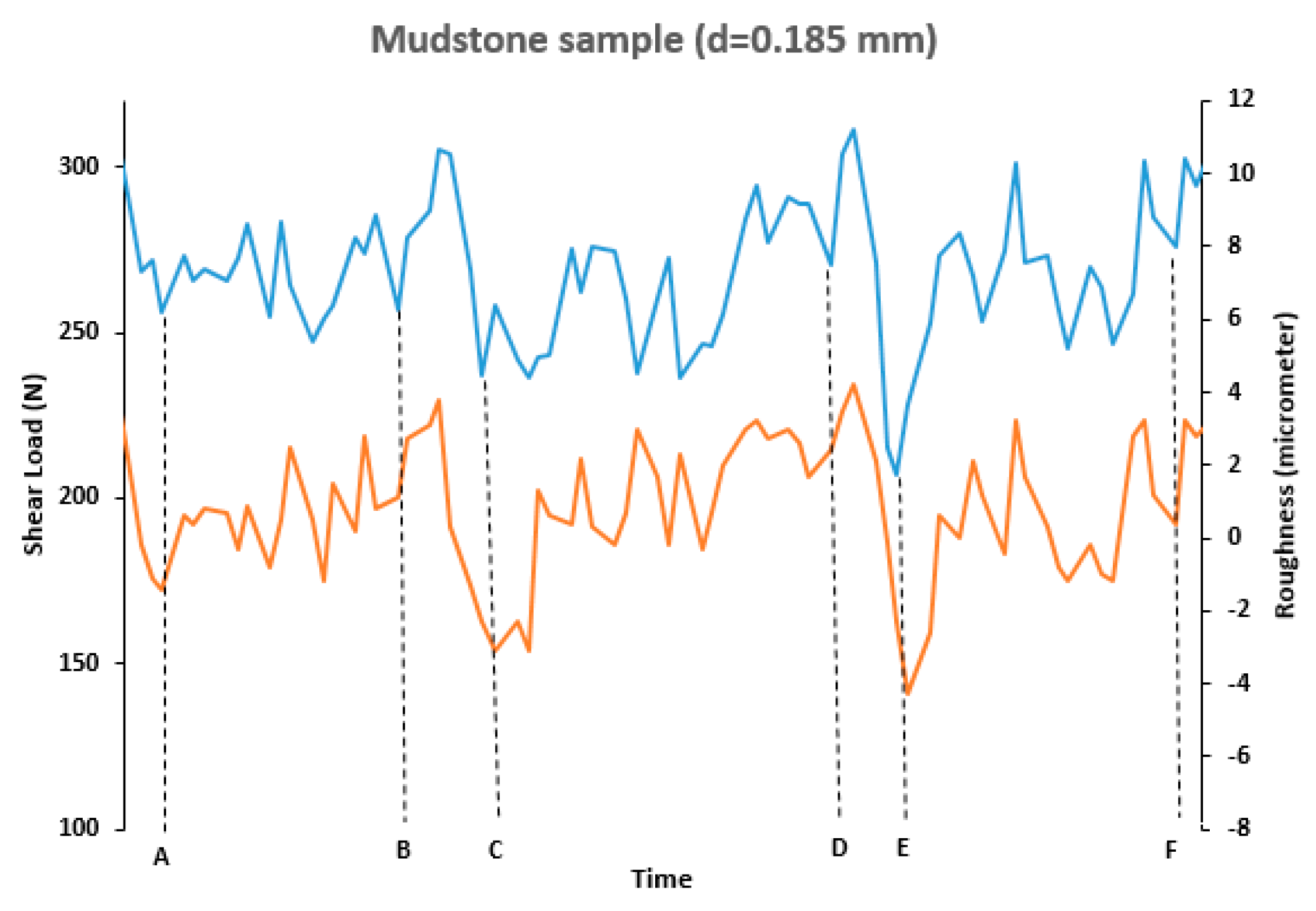
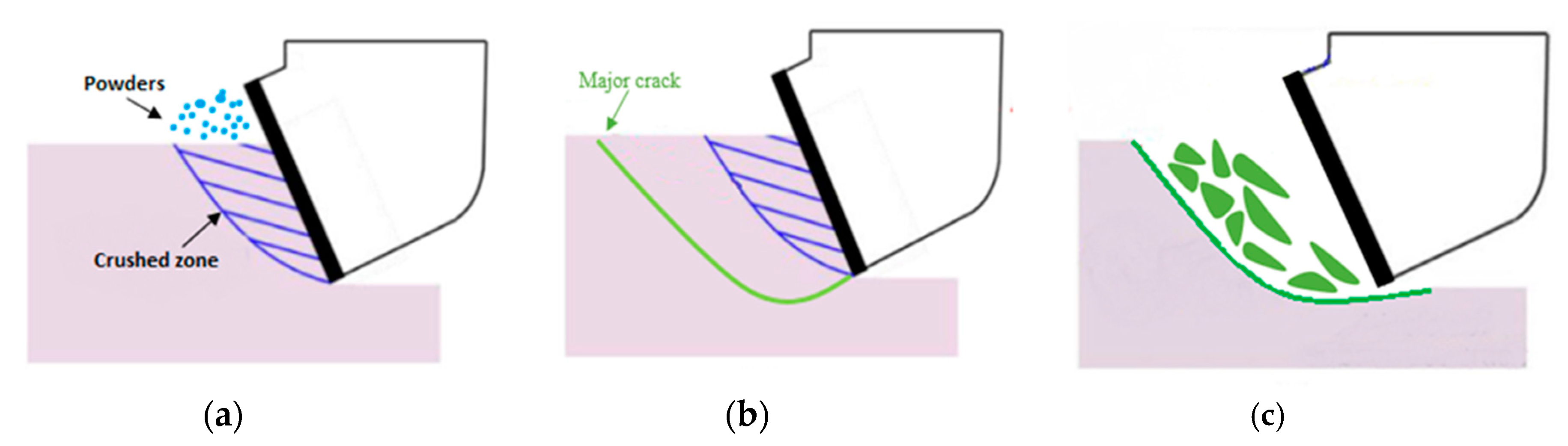
Figure 6 represents the shear force and the surface roughness of mudstone rock sample values during a scratch test. At the beginning of time A, the cutter starts to compress the surface and creates a crushed zone until time B (see Figure 7a). During this time interval, cutting force and surface roughness numbers exhibit small fluctuations. After this period, the cutting force rises and reaches its peak between time B and C. As a result, a major crack defining the chip in front of the cutter is formed (see Figure 7b). Another proof for this explanation is seen in the change of roughness magnitude. The surface roughness value stays within a small range before chipping begins, but the sharp increase of the cutting force causes a big altitude change in surface asperities. After a crack is expelled from the rock surface, the cutting force reduces, and the cutter moves very fast in a short time due to inertia (see Figure 7c). This chip removal leads to deep damage on the groove surface, so it makes for a significant change in surface roughness in this part. After time C, this process as outlined above repeats. In this graph, the time interval between A and B, C and D, and lastly E and F illustrate the ductile failure mode (a smooth cut path), while the results at intervals from B to C and D to E display examples of brittle failure (the groove surface is rough).

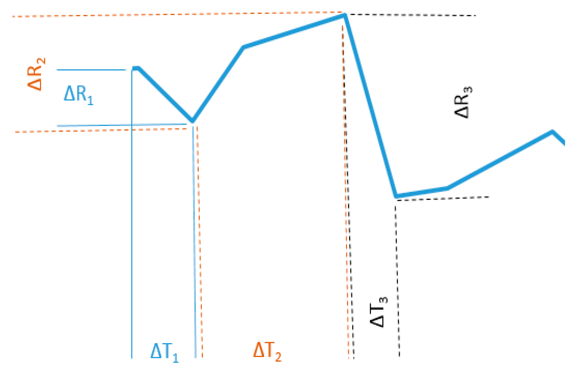
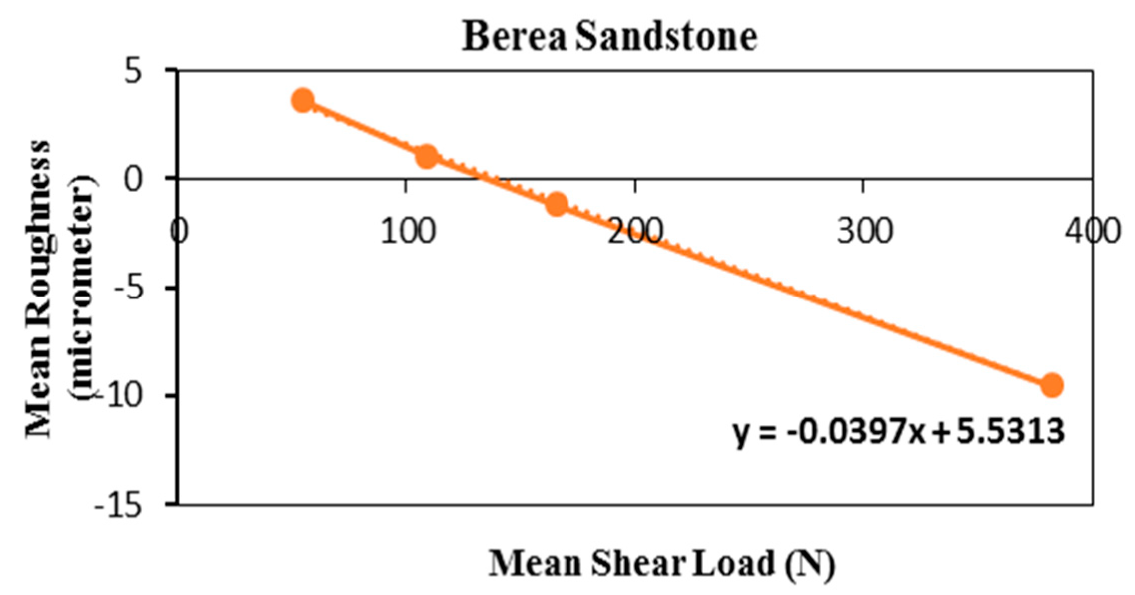
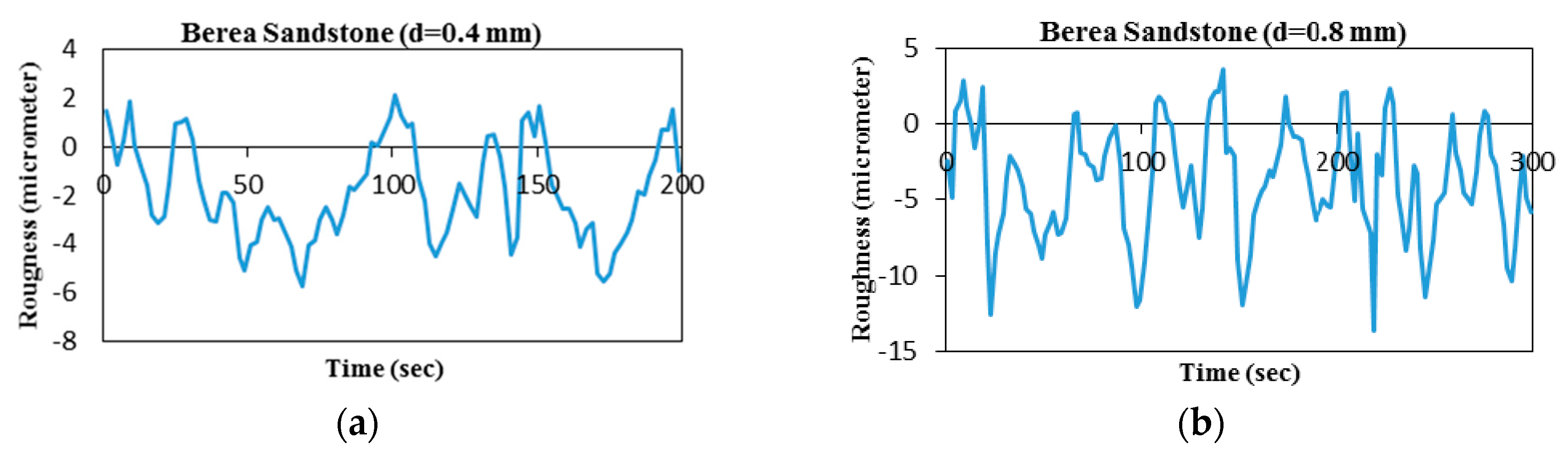
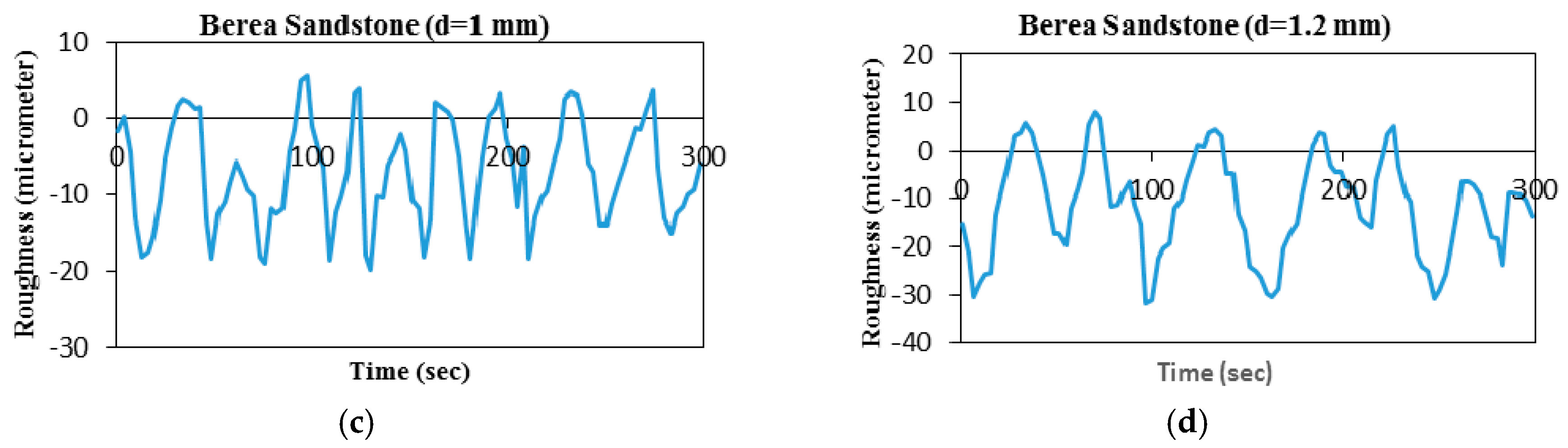
Based on the extensive scratch tests conducted in this research, the surface roughness can be realized as another method for delineating the rock cutting mechanism. It is seen that small asperities on the cut surface and long process time are characteristics of the strength-driven mode. On the contrary, the groove surface has big fluctuations over a short distance/time when the fracture-driven mode is dominant. As shown in Figure 8, $\Delta R$ and $\Delta T$ show the scratched surface altitude difference and the time difference, respectively. The ratio of $\Delta R$ and $\Delta T$ illustrates an average change in the surface roughness is defined as follows:

$$R_t= \frac{\mathsf{\Delta }R}{\mathsf{\Delta }T} ,$$

(11)

It is notable that, due to the discontinuous nature of the measured forces, it is not possible to take its derivative. The value of $R_t$ depends on the failure mode. When the magnitude of $R_t$ is small and cuttings are in the form of powder, the failure mechanism occurs in the ductile mode. If the failure mode is fracture-driven and cuttings are chunks, the value of $R_t$ is high. As shown in Figure 8, $R_t{}_1$ and $R_t{}_2$, which have small surface asperities change over a long time, exemplify the ductile failure mode. On the other hand, $R_t{}_3$ is the biggest and shows features of the fracture-driven failure.

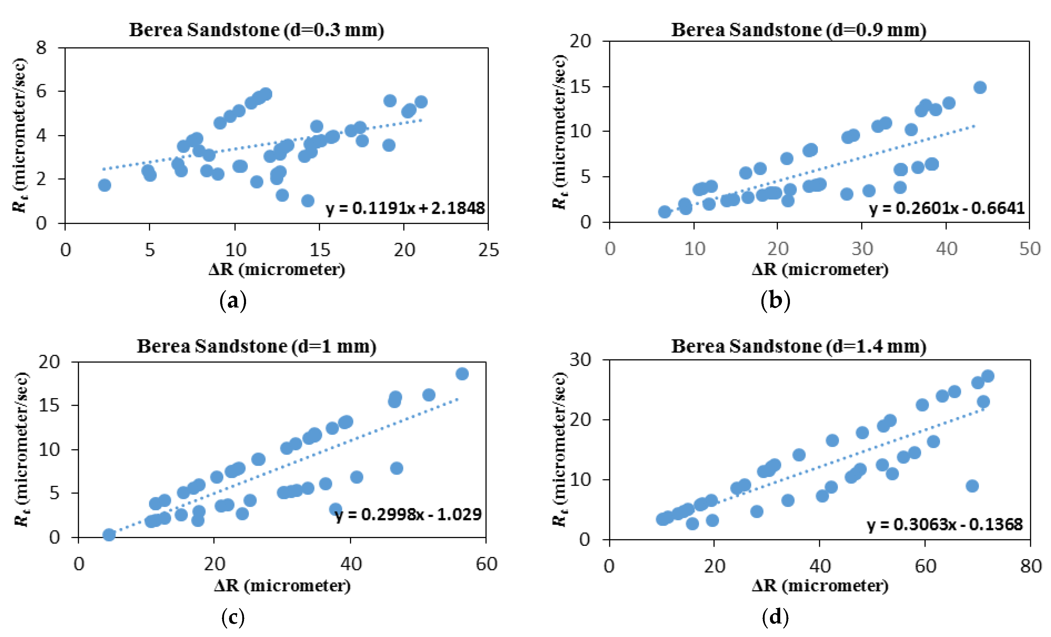
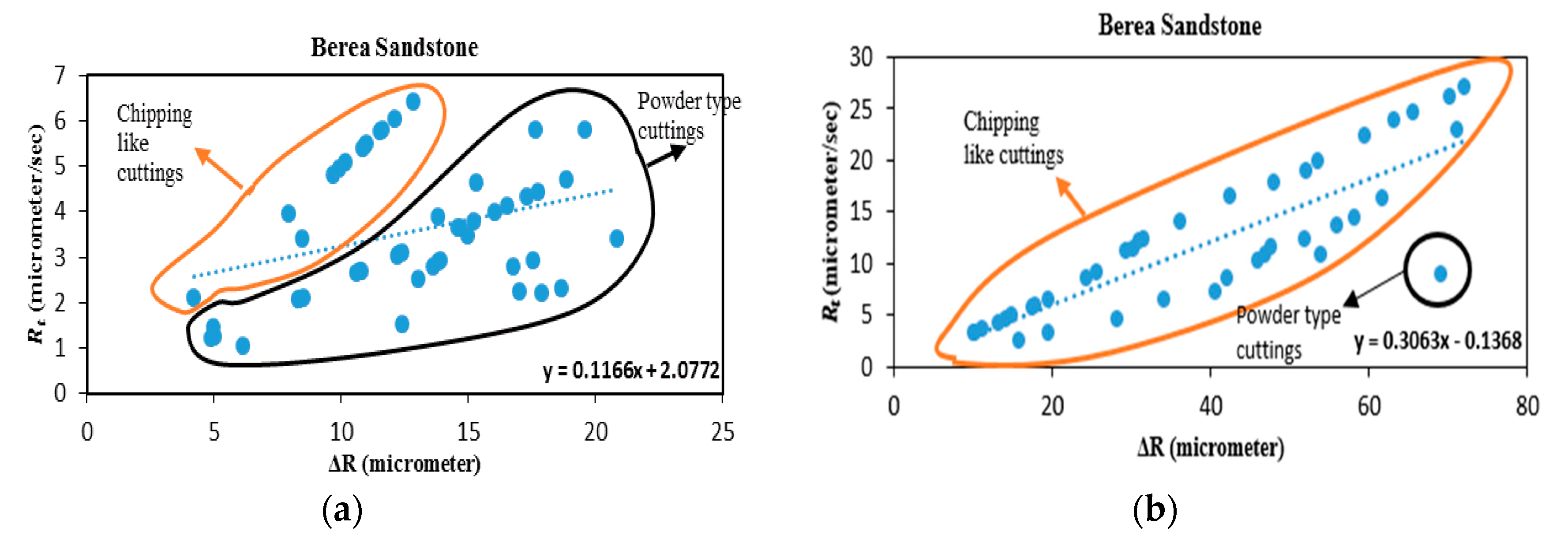
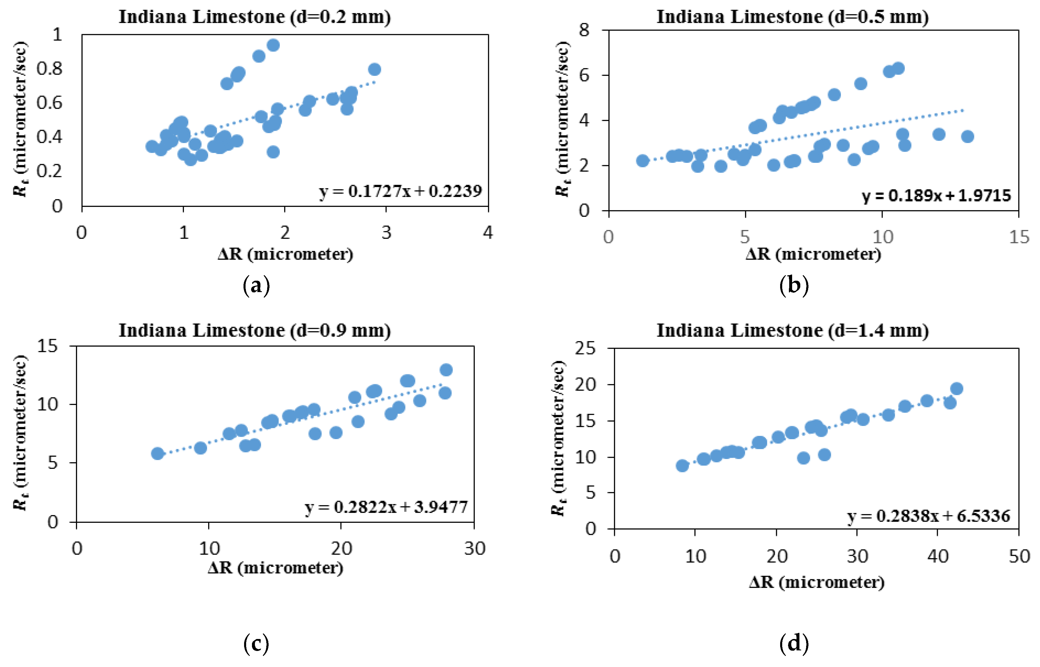
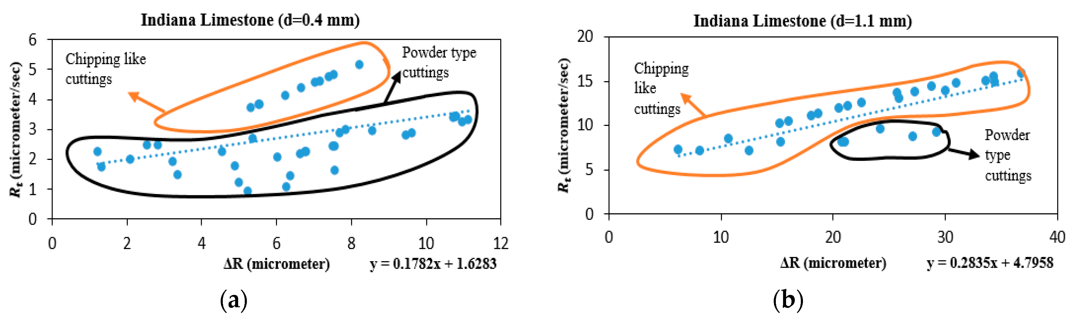
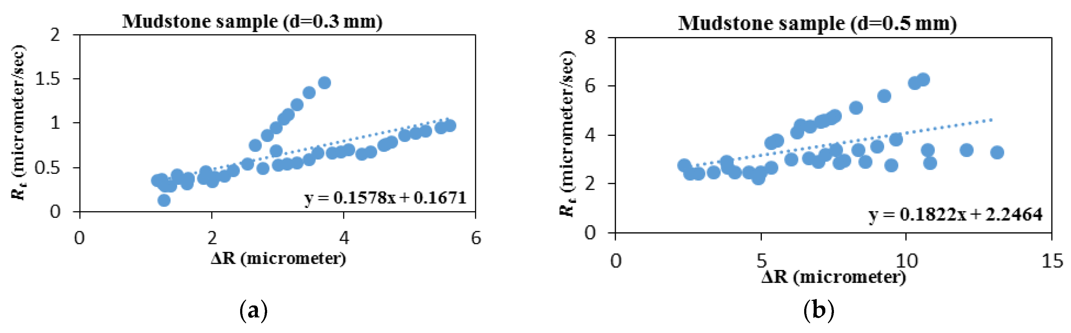
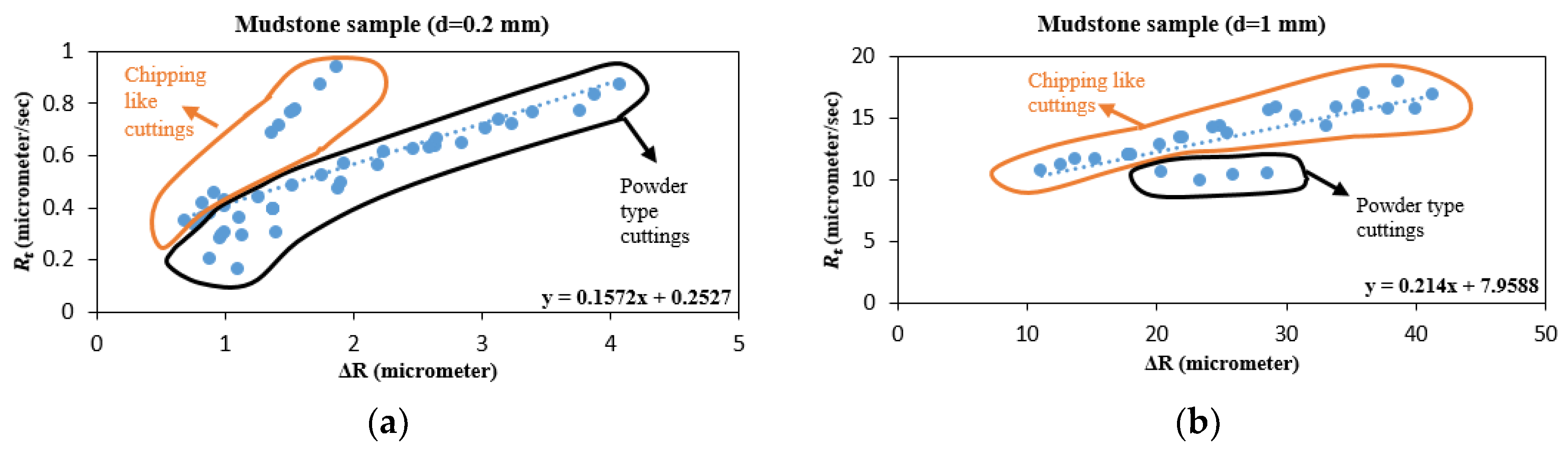
It is expected that data points separate into two trends in the $R_t$ and ΔR graph. The upper trend of this graph belongs to chunk-like cuttings since the roughness of cut surface changes remarkably over a short time. The lower group represents powder type cuttings during the rock cutting process, owing to the smooth surface roughness. In the small DOC of the rock cutting process, lower part points would dominate. However, this density falls off, and some dots show up on the upper side with rising DOC. This trend continues until reaching the transition point. 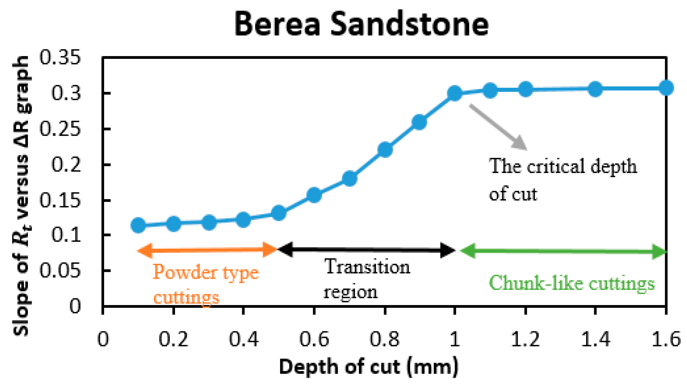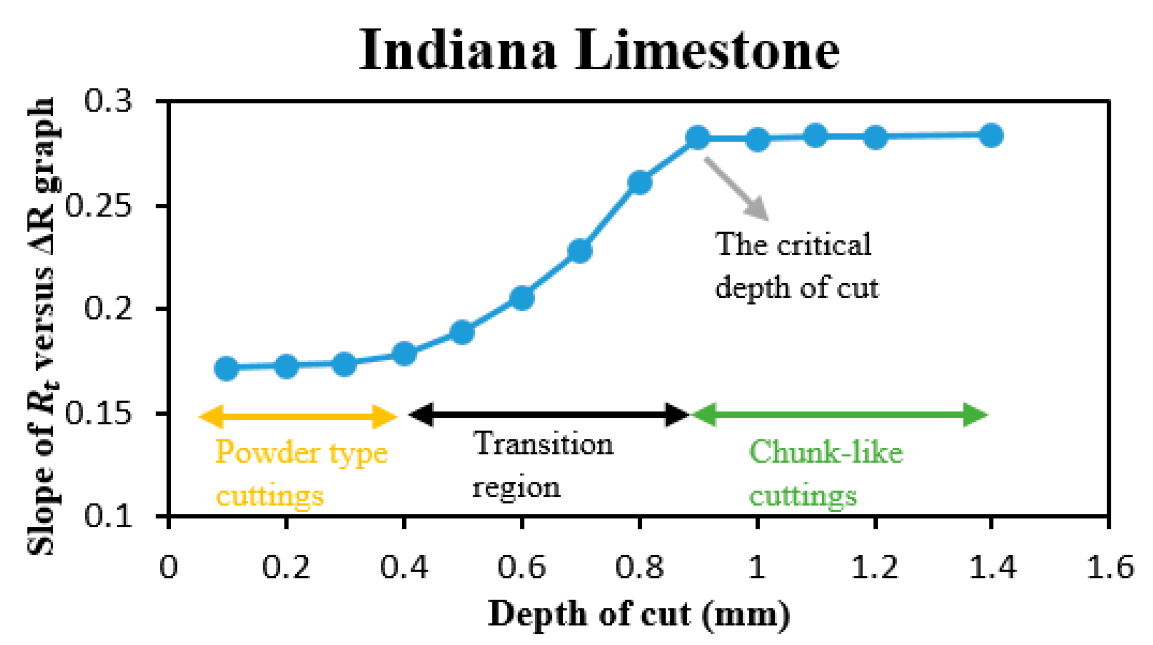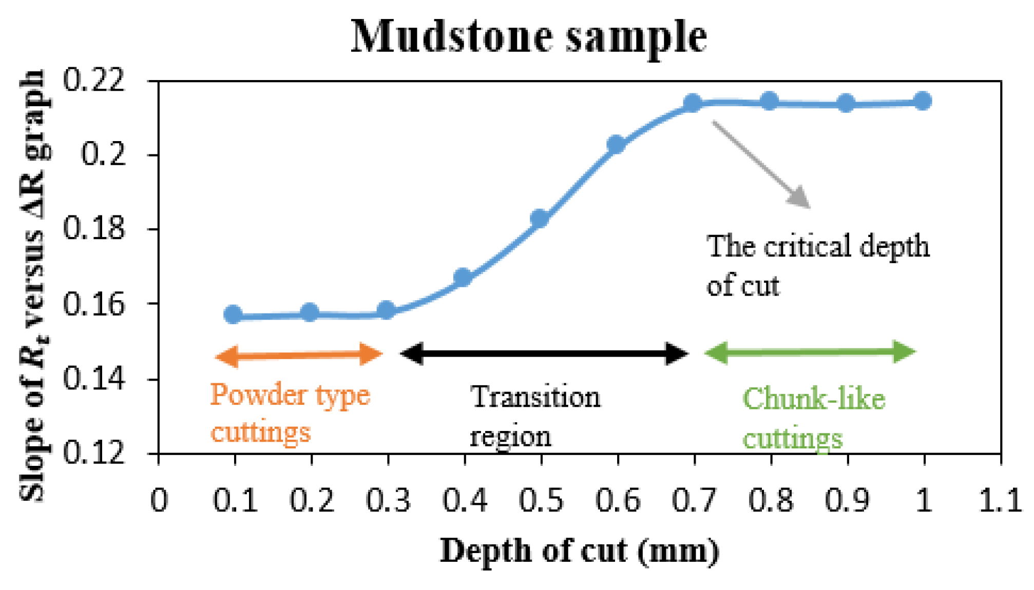Beyond the critical DOC, upper side points are much denser than the lower side ones (see Figure 9). The number of the chips is negligible at small DOCs, where so the slope remains almost steady. Later, chunk-like cuttings start to dominate the graph and the slope of the line goes up sharply until reaching the critical DOC. Then, the slope levels out again because the failure mechanism turns to the brittle mode (no powder cutting). As a result, the slope of $R_t$ and $\Delta R$ chart versus the DOC graph is another way to determine the critical DOC.

3. Experimental Setup

This research required extensive laboratory tests in parallel with numerical simulations to investigate the failure mechanism of rock cutting and the transition point of rock, but the resultant roughness of the cut surface has not been included in the analysis, albeit measuring roughness requires a lesser amount of instrumentation in comparison to force measurements. What is more, measuring surface roughness can be done repeatedly after the test and does not require any complexity. To validate the roughness approach, experimental studies into different rocks have been carried out and reported here. The laboratory tests were conducted with the scratch test system build by TerraTek, now a Schlumberger Company. This device has a fixed slant to hold a blunt or sharp cutter. The DOC and the cutter velocity are controlled and kept constant while the normal and shear forces required for the scratch are measured and recorded accurately over the range of 0 to 2000 N.

In this study, 5 mm width rectangular-shaped sharp cutters are utilized to run tests similar to what has been used by Richard [5], who claimed that this cutter width gives more sensitive results at shallower depths. The back-rake angle of the cutter is fixed at 15°. The experimental results in Richard et al. [10] prove that the scratch test results are close to the UCS test outcomes when the back-rake angle varies between 10° and 20°. The rectangular-shaped cutter gives a better correlation between the scratch test and the uniaxial compression strength test, due to less significant end-effects.

Three common types of sedimentary rocks are scratched in this work: Berea sandstone, Indiana Limestone, and Mudstone (shale) sample with the properties listed in

Table 1. Mechanical and petrophysical properties of rock samples used in this study.

Rock Type	q (Mpa)	Ø (%)	ρ (kg/m3)	K (mD)	E (Gpa)	ν
Berea Sandstone	44.8	19.46	2170	115	13.2	0.2
Indiana Limestone	30.2	16	2290	4	16.1	0.14
Mudstone (Shale) Sample	23	1.05	2300	2.22	15.06	0.238

. All rock samples are drilled with a 1″ diameter hole saw drill bit, and prepared as 5 to 20 mm core samples, so cut grooves have a U-type profile in these experiments.

4. Results and Discussion

4.1. Berea Sandstone

The scratch tests are conducted with different DOCs. First, the Berea sandstone sample is scratched by a rectangular sharp cutter at 0.15, 0.175, 0.2, and 0.3 mm depths, then shear forces and corresponding surface roughness are recorded during these tests are presented in Figure 10. These results not only follow the approach of Detournay and Defourny [12] (i.e., the mean tangential load increases with the DOC) but also reveal the inverse relationship between the DOC and groove asperities (see Figure 11a,b). For example, one may notice that when changes in shear force values during scratching the rock sample are small, the cut surface is smooth, but the roughness value of the groove shows notable fluctuations while the tangential forces display large fluctuations. Another important outcome of these tests is that roughness and the cutting force follow the same pattern during the cutting process. Additionally, these lab results illustrate that the averaged roughness value also follows a downward trend with increasing DOC (see Figure 11b).

In order to verify the ideas proposed in the previous section for determining the transition point for the Berea sandstone, the $R_t$ (the average change in a surface roughness) value is calculated for each measurement point along the scratch path. Zhou and Lin [18] reported that the critical point of Berea sandstone is about 1 mm. Because of the limitation of our scratch test system, i.e., the capacity of the load sensor is limited to 2000 N, the experimental tests could not go beyond the 0.3 mm DOC. To overcome this limitation, another method is used to estimate the scratched groove roughness for each DOC.

Figure 12 indicates an inverse relationship between the mean roughness of the scratched path and the cutting force. The equation illustrated in the graph can be used to calculate the average asperity of the rock surface for each DOC. In the literature, the averaged tangential force has been published for different DOCs in Berea sandstone. The combination of the equation shown in Figure 12 and the mean shear load from published articles can be used to calculate the mean surface roughness value for various DOCs. After finding the average asperity of the groove surface, the scratched rock surface can be reproduced by employing the Weierstrass-Mandelbrot model for the given DOC.

Mehrami et al. [23] used the Weierstrass-Mandelbrot model to generate a rough surface profile z(x), where the altitude along the scratched groove surface at any point x is expressed as:

$$z\left(x\right)=L{\left(\frac{G}{L}\right)}^{\left(D-1\right)}{{\displaystyle \sum }}_{n=0}^{\infty }\frac{\cos \left(\frac{2\pi v^{n}x}{L}\right)}{v^{\left(2-D\right)n}},$$

(12)

where L and v represent the sample length and a scaling parameter, respectively, and G represents the fractal roughness parameter arrived by changing the distance between the peaks and valleys on the surface. In this formula, D, which controls fluctuation frequency, varies between 1 and 2, but the suggested number is 1.5 [24], and v is always bigger than one otherwise, this formula gives a flat surface. Rough surfaces are estimated with higher values of D and G.

In our paper, the cutting speed is assumed to be constant as set in the device, so the above formula can be modified to replace coordinates with the corresponding time in order to compare the surface roughness with the force magnitudes, which are acquired as functions of time. In the new form, z(τ) represents the height of groove asperity at time τ:

$$z\left(\tau \right)=T{\left(\frac{G}{T}\right)}^{\left(D-1\right)}{{\displaystyle \sum }}_{n=0}^{\infty }\frac{\cos \left(\frac{2\pi v^n\tau }{T}\right)}{v^{\left(2-D\right)n}}$$

(13)

where T is the total cutting time. In other words, z(τ) is the instantaneous roughness below the cutter.

As mentioned previously, the average groove roughness has been estimated using the correlation derived from Figure 12. The mean tangential force is then found from published data in the literature for different DOCs. Using these average groove roughness values, the rough surfaces, whose cutting time is 200 s for shallow depths and 300 s for deep depths, are generated using Equation (13) by altering G and D values. Rough surfaces have been generated for different DOCs ranging from 0.1 mm to 1.5 mm in 0.1 mm increments (Figure 13). Figure 13 also illustrates that the grooved surface is much smoother at small DOCs, and the roughness change per unit of time is small. On the other hand, the high average frequency of surface roughness change is an indicator of the brittle failure mechanism at high DOCs.

The $R_t$, which presents the average change in the surface roughness, is calculated along the grooved path and then $R_t$ versus $\Delta R$ graphs are used to better illustrate surface topographic variations (see Figure 14). If $R_t$ and $\Delta R$ are small, it means that the cutter scratches the rock surface in powders, which is a result of the ductile mode failure. As illustrated in Figure 14a, shallow DOCs have small $R_t$ values and this number increases with rising the DOC. On the other hand, large chips are the main components of debris when the DOC is deep enough (see Figure 14c,d). As explained previously, the groove surface altitude change between two points has a positive correlation with increasing DOC. Figure 14 also confirms that ΔR varies in the range of 0–20 µm at small DOCs, whilst it reaches to about 80 µm when the depth of cut increases.

In addition, sometimes DOC variations do not affect the slope of the $R_t$ versus ΔR graph, or it shows a significant rise at only few points. This behavior depends on cutting type during the cutting process. At shallow depths, powder is the dominant cutting type, and the number of chunk-like cuttings is small, so the slope of this graph remains almost constant even though $R_t$ and $\Delta R$ values change constantly. However, this trend diminishes with an increase in the number of chunk-like cuttings. Beyond the transition point, the number of chunk-like cuttings increases, and the slope experiences a sharp increase. In parallel, the groove surface roughness shows significant changes in a short time. These variations further increase as DOC rises. The upward trend of $R_t$ versus $\Delta R$ ends after complete transition to brittle mode, so $R_t$ and $\Delta R$ maintain this trend. Another important observation from this graph is that there are two different linear trends, representing powder cutting tests and chunk-like cutting tests, so the cutting mode transition happening with the rising DOC is crucial in identifying the failure mechanism transition in the rock cutting process (Figure 15).

The slope of the $R_t$ versus $\Delta R$ remain almost constant at small DOCs, then experiences a sharp increase, before reaching an almost constant value as DOC is getting deep enough (Figure 16). Therefore, the rock cutting process can be divided into three parts. First, the cutter crushes the rock surface at shallow DOCs and cuttings are in the form of powder (chunk-like cutting is seen rarely). Therefore, the slope of the $R_t$ versus $\Delta R$ line graph does not change until a considerable amount of chip cuttings are expelled. In the transition mode, powder and chunk-like cuttings are generated simultaneously. The slope of the $R_t$ versus $\Delta R$ remains almost constant in this period because cuttings are almost chips, and so there is a similar increase in $R_t$, the average change in the surface roughness, and $\Delta R$, surface roughness difference. In other words, $R_t$ is independent of time in this period and a height difference between two points of the cut surface is the only component that changes this value. Similarly, in their work, Pang and Goldsmith [25] categorized the cutting process in three sections: a crushed region, a minor crack region, and a major crack region.

The last but most striking result to emerge from these laboratory tests is the alternative method for determining the transition point for the Berea sandstone cutting process. As mentioned previously, the rock scratch process is divided into three periods. In the literature, the critical DOC refers to the point in which the brittle failure mode starts. It is well known that the major cutting sample of this mode is a chip. This explanation refers to the intersection point of the second and third zone, as shown in Figure 16. Because the content of debris consists of chunk-like cuttings after this depth, the critical depth of point for Berea sandstone is found as 1 mm in this work. This result confirms previous results in the literature. Nicodeme [4] used DD method and calculated this point between 1 mm and 1.1 mm, while Zhou and Lin [18] found this value to be about 1 mm by employing the size effect equation.

4.2. Indiana Limestone

Indiana limestone is the second type of rocks studied in this research. The rock is cut at depths of 0.175, 0.18, 0.185, and 0.19 mm. As illustrated in Figure 17, there is a positive correlation between the tangential force and surface roughness in our conducted tests, which is like Berea sandstone. In other words, they have nearly similar line paths along the entire cut. Additionally, the Indiana limestone scratch test results show that the mean grooved surface asperity decreases as DOC increase. Additionally, this positive correlation between the tangential force and the DOC confirms DD model, which proposes that the mean tangential load rises linearly with increasing DOC (see Figure 18). It is also crucial to note that the mean values of shear force and average surface asperity have an inverse correlation (see Figure 19).

The load sensor capacity of our scratch test device cannot allow the Indiana limestone sample to be cut at deep DOCs, even though the transition point of Indiana limestone has been estimated to be over 0.7 mm by Che et al. [21]. The mean tangential component of measured load results for this rock is shown in Figure 19, which gives a correlation between the mean shear load and the mean surface roughness. Hence, the equation is represented in Figure 19 can be used to find the average groove asperities for different DOCs. These average numbers are used to estimate groove surfaces whose total cutting time is 300 s, ranging from 0.1 to 1.4 mm DOCs, by employing the modified Weierstrass-Mandelbrot model (see Equation (13) and Figure 20). The main takeaway from these figures is that the average roughness is small at shallow DOCs, while the altitude of the groove surface shows strong fluctuations in the case of large DOCs.

The $R_t$ versus $\Delta R$ is plotted from 0.1 mm to 1.4 mm to demonstrate the evolution of the rock cutting mechanism of Indiana limestone (see Figure 21). Similar to Berea sandstone, the slope of the $R_t$ versus $\Delta R$ graph, $R_t$ and $\Delta R$ are small at shallow DOCs. In other words, the cutter has a small impact on the rock surface, so the surface would be smooth. $R_t$ and $\Delta R$ show a gradual growth with increasing DOC, but the slope remains almost the same for a while. Even though these three parameters show a significant increase between 0.4 and 0.9 mm DOCs, the slope of this graph again becomes constant above 0.9 mm DOC.

This behavior can be explained using the debris type of the cutting process. At the beginning, there are powder type cuttings throughout the entire test. Powder particles are too small; thus, it cannot cause much resistance against the cutter movement. As a result, small cutting force fluctuations would lead to small changes in $R_t$ and $\Delta R$ and, consequently, the slop of the graph (see Figure 22). However, the chipping type deformation causing significant surface changes after 0.4 mm DOC and, as the result, the slope of the graph goes up significantly until it reaches the critical DOC, which is the endpoint of the transition zone. In this region, powder and chunk-like cuttings are produced simultaneously. Beyond this depth, cutting debris consists mainly of chips and $R_t$ and $\Delta R$ show similar changes. As detailed in Figure 22, the critical DOC for Indiana limestone is found to be 0.9 mm. This value is consistent with previous results. Che et al. [21] used a high-speed camera to determine the transition DOC in Indiana limestone samples ranging between 0.7 mm and 1 mm.

Lastly, Figure 23 illustrates two examples of the $R_t$ versus $\Delta R$ graphs to show cutting type changes with increasing DOC. The amount of powder type cuttings indicates that the failure mechanism is ductile at d = 0.4 mm, while chips are seen, although their number is few. After passing the critical DOC, this situation reverses, and the chunk-like cuttings comprise the majority of the debris. As seen in Figure 23b, the amount of powder type cuttings is negligible compared to the number of chunk-like cuttings at deep DOCs.

4.3. Mudstone (Shale) Sample

In the last part of the experimental efforts, the single cutter scratch test is carried out on mudstone specimens at 0.175, 0.18, 0.185, and 0.19 mm DOCs. The laboratory test results on this rock sample are presented in Figure 24. This data also shows that the tangential force and cut groove surface lines undergo similar changes during the scratching of the mudstone sample.

It is known that the mean cutting force increases with the rising DOC; this relation is represented in Figure 25a. Additionally, the average surface asperity has been calculated for each DOC to determine the relationship between the mean cut groove roughness and DOC (as seen in Figure 25b). A remarkable result to emerge from these experimental results is that there is an inverse correlation between the average shear load and the mean surface asperity during the mudstone cutting process, similar to that of Berea sandstone and Indiana limestone scratch test results (see Figure 26).

As mentioned previously, our tests suffers from the capacity limitation of the load sensor. This drawback prevents running experimental scratch test above the 0.19 mm DOC for this type of rock. At this point, the reported mean tangential force for each DOC in Mudstone sample in the literature is employed and combined with the correlation shown in Figure 26 to obtain the average surface asperity for each DOC. Then, Equation (13) is used to replicate cut rock surface asperities from 0.1 mm to 1 mm DOC. The resultant rock surfaces for DOC ranging from 0.1 mm to 1 mm are generated (e.g., see Figure 27). Fluctuations are small at shallow depths, while the rock surface experiences steep fluctuations at deep DOCs.

Based on our data, it can be easily verified that the change in groove roughness depends on DOC, which is the main motivation in this paper. To assess its validity, $R_t$ (the average change in the surface roughness) and $\Delta R$ (the difference in surface roughness between two points) have been calculated for various DOCs (see Figure 28). It is plausible that these values will grow as the DOC increases. Moreover, they are a good indicator in defining the failure regime of rock. Additionally, the slope of the $R_t$ vs. $\Delta R$ stays constant at the beginning, before increasing sharply in the middle, and then leveling out again at the end.

Surface asperity change ($\Delta R$) and the average change in the surface roughness ($R_t$) are determined along the entire groove to verify the validity of the roughness model; the results are represented in Figure 28. This graph also illustrates the effect of the rising DOC on the rock cutting mechanism. Like previous tests, the mudstone specimen has the lowest $R_t$ and $\Delta R$ at shallow depths due to the small size of debris. Even though these two values experience moderate growth from 0.1 mm to 0.3 mm DOC, the slope of the $R_t$ vs. $\Delta R$ remains almost the same. At this stage, the cutter crushes the surface of the mudstone into powder type cuttings. Here, chipping like cuttings are rarely seen. Beyond 0.4 mm DOC, $R_t$, $\Delta R$, and the slope of the $R_t$ vs. $\Delta R$ show an upward trend. Particularly, the slope of the $R_t$ vs. $\Delta R$ rises sharply up to 0.7 mm DOC. Between 0.4 and 0.7 mm DOC, a new cutting type appears, the cutter not only crushes the rock surface but also produces chips while cutting the mudstone sample. Even though the number of chips is few when DOC is 0.4 mm. In the last part of the slope, $R_t$ vs. $\Delta R$ again remains steady after the DOC of 0.7 mm. This indicates that the cutting type turns almost to chunk-like cuttings. Beyond this cutting depth, $R_t$ and $\Delta R$ have approximately the same trend, so the slope of the plot shows just minor changes.

As mentioned previously, the slope of $R_t$ vs. $\Delta R$ gives us a clue to determine the failure mechanism and the relevant transition point. The critical depth of the mudstone sample is found to be 0.7 mm in this work. The roughness approach is the first model to determine the critical DOC of the shale rock specimen (see Figure 29). This number is meaningful when the tangential force and surface roughness values of the mudstone sample are compared to the Berea sandstone and the Indiana limestone results at similar DOCs. For instance, the mean shear load value is 288.5 N for the mudstone sample (DOC = 0.175 mm), while this load is 108.5 N at the same DOC for the Berea sandstone sample. Namely, more energy is required to cut the mudstone sample at the same depth. As a result of this difference, the mechanical cutter is exposed to damage at large DOCs in the mudstone surface; consequently, this rock shows a bigger absolute value of surface asperity at the same DOC. Therefore, it experiences major cracks at the smaller DOC along the cutting process, which causes shallow critical DOC.

Another advantage of $R_t$ vs. $\Delta R$ is the fact that this graph represents the number of chunk-like cuttings versus powder type cuttings, so the dominant failure mode of the cutting process can be easily identified. It is apparent from Figure 30 that powder is the major cutting type when the DOC is 0.2 mm for this sample. On the other hand, at the 1 mm cutting depth, the powder-type cuttings are negligible.

5. Conclusions

In order to determine the critical DOC for transition from ductile to brittle failure mode and vice versa, a variety of scratch tests were conducted in this work. Previous methods to determine this transition point were mainly concerned about analyzing shear and normal forces acting on the cutter. Our studies show that the cutter damage to the surface of the rock when deeper than the critical DOC depends on the rock type. Therefore, this behavior demonstrates another method to identify the transition point. This new roughness approach is verified using a combination of laboratory tests and numerical analysis to determine the transition point of rock cutting. The greatest achievement of this model is that the critical depth of a shale sample has been determined for the first time. The results show that the surface roughness behaves similar to the tangential measured forces. The laboratory tests prove that the cut groove surface is smooth and that the cutting type is powder at the shallow depths. On the contrary, the altitude difference between two points on the rock surface is high and the cutting type becomes chips when the scratching depth gets deep.

References

1. Liu, W.; Zhu, X.; Jing, J. The analysis of ductile-brittle failure mode transition in rock cutting. J. Pet. Sci. Eng. 2018, 163, 311–319. [Google Scholar] [CrossRef]
2. Haywood, M. Ductile failures in reinforced concrete beams strengthened using fibre reinforced plastics. In Proceedings of the 6th Austroads Bridge Conference, Perth, Australia, 12–15 September 2006. [Google Scholar]
3. Walker, S.; Li, J. The effects of particle size, fluid rheology, and pipe eccentricity on cuttings transport. Soc. Pet. Eng. 2000. [Google Scholar] [CrossRef]
4. Nicodeme, P. Transition between Ductile and Brittle Mode in Rock Cutting, Rapport de Stage d’option Scientifique; Ecole Polytechnique: Palaiseau, France, 1997. [Google Scholar]
5. Richard, T. Determination of Rock Strength from Cutting Tests; The University of Minnesota: Minneapolis, MN, USA, 1999. [Google Scholar]
6. Jaime, M.C.; Zhou, Y.; Lin, J.-S.; Gamwo, I.K. Finite element modeling of rock cutting and its fragmentation process. Int. J. Rock Mech. Min. Sci. 2015, 80, 137–146. [Google Scholar] [CrossRef] [Green Version]
7. Bifano, T.G.; Fawcett, S.C. Specific grinding energy as an in-process control variable for ductile-regime grinding. Precis. Eng. 1991, 13, 256–262. [Google Scholar] [CrossRef]
8. Molloy, P.; Schinker, M.G.; Doll, W. Brittle fracture mechanisms in single point glass abrasion. In Proceedings of the Hague International Symposium, Houston, TX, USA, 1–6 March 1987; pp. 81–88. [Google Scholar]
9. Adachi, J.I.; Detournay, E.; Drescher, A. Determination of rock strength parameters from cutting tests. In Rock Mechanics, Tools and Techniques, Proceedings of the 2nd North American Symposium of Rock Mechanics, Montreal, QC, Canada, 19–21 June 1996; Aubertin, F.H.M., Mitri, H., Eds.; CRC Press: Boca Raton, FL, USA, 1996. [Google Scholar]
10. Richard, T.; Dagrain, F.; Poyol, E.; Detournay, E. Rock strength determination from scratch tests. Eng. Geol. 2012, 147, 91–100. [Google Scholar] [CrossRef]
11. Ersoy, A.; Buyuksagic, S.; Atici, U. Wear characteristics of circular diamond saws in the cutting of different hard abrasive rocks. Wear 2005, 258, 1422–1436. [Google Scholar] [CrossRef]
12. Detournay, E.; Defourny, P. A phenomenological model for the drilling action of drag bits. Int. J. Rock Mech. Min. Sci. Geoméch. Abstr. 1992, 29, 13–23. [Google Scholar] [CrossRef]
13. Zhu, X.; Liu, W.; He, X. The investigation of rock indentation simulation based on discrete element method. KSCE J. Civ. Eng. 2017, 21, 1201–1212. [Google Scholar] [CrossRef]
14. Shojaei, A.; Taleghani, A.D. A Continuum Damage Model to Predict Bit Performance Based on Single Cutter Experiments; International Society for Rock Mechanics and Rock Engineering: Salzburg, Austria, 2015. [Google Scholar]
15. Bazant, Z.P.; Hasegawa, M.; Mazars, J. Size effect in Brazilian split-cylinder tests: Measurements and fracture analysis. ACI Mater. J. 1991, 88, 325–332. [Google Scholar]
16. Van Mier, J.G. Concrete Fracture: A Multiscale Approach; CRC Press: Boca Raton, FL, USA, 2012. [Google Scholar]
17. Bazant, Z.; Le, J. Probabilistic Mechanics of Quasibrittle Structures: Strength, Lifetime, and Size Effect; Cambridge University Press: Cambridge, UK, 2017; pp. 1–21. [Google Scholar] [CrossRef]
18. Zhou, Y.; Lin, J.-S. On the critical failure mode transition depth for rock cutting. Int. J. Rock Mech. Min. Sci. 2013, 62, 131–137. [Google Scholar] [CrossRef]
19. He, X.; Xu, C.; Peng, K.; Huang, G. On the critical failure mode transition depth for rock cutting with different back rake angles. Tunn. Undergr. Space Technol. 2017, 63, 95–105. [Google Scholar] [CrossRef]
20. He, X.; Xu, C. Specific energy as an index to identify the critical failure mode transition depth in rock cutting. Rock Mech. Rock Eng. 2016, 49, 1461–1478. [Google Scholar] [CrossRef]
21. Che, D.; Han, P.; Peng, B.; Ehmann, K.F. Finite element study on chip formation and force response in two-dimensional orthogonal cutting of rock. In Proceedings of the International Manufacturing Science and Engineering Conference ASME, Detroit, MI, USA, 3 October 2014. [Google Scholar]
22. Cheng, Z.; Sheng, M.; Li, G.; Huang, Z.; Shi, H.; Dai, X.; Guo, Z. Cracks imaging in linear cutting tests with a PDC cutter: Characteristics and development sequence of cracks in the rock. J. Pet. Sci. Eng. 2019, 179, 1151–1158. [Google Scholar] [CrossRef]
23. Mehrabi, A.R.; Rassamdana, H.; Sahimi, M. Characterization of long-range correlations in complex distributions and profiles. Phys. Rev. E 1997, 56, 712–722. [Google Scholar] [CrossRef]
24. Wang, S.; Shen, J.; Chan, W.K. Weierstrass-Mandelbrot Function; Wolfram MathWorld: St. Louis, MO, USA, 2006; pp. 1–7. [Google Scholar]
25. Pang, S.S.; Goldsmith, W. Investigation of crack formation during loading of brittle rock. Rock Mech. Rock Eng. 1990, 23, 53–63. [Google Scholar] [CrossRef]
Figure 1. (a) Ductile mode scratching (d = 1 mm) and (b) brittle mode scratching (d = 4 mm) for Berea Sandstone [5].
Energies 13 04496 g001
Figure 2. (a) The cutting force versus depth of cut (DOC) graph for Rhune sandstone [4]. The averaged peak shear load increases linearly up to the transition point. d c is the depth where the linearity ends. Here, the critical DOC is found at about 0.4 mm Rhune sandstone. (b) The nominal stress-DOC graph for Rhune sandstone [18]. Two dashed lines intersect at 0.8 mm, which is the critical DOC.
Energies 13 04496 g002
Figure 3. The specific cutting energy values throughout the rock cutting process: (a) Tuffeau limestone, (b) Savonnières limestone [20]. These graphs show the evolution of the specific energy versus d 4 / 3 . The specific energy does not change with the DOC in the ductile mode.
Energies 13 04496 g003
Figure 4. Surface roughness of Berea sandstone sample after the cutting process: (a) DOC = 0.1 mm, (b) DOC = 0.4 mm. Both pictures are sharing the same scale but roughness cannot be noticed by naked eyes.
Energies 13 04496 g004
Figure 5. The shear force and the groove roughness variation during the cutting process: (a) Berea sandstone (DOC = 0.2 mm), (b) Mudstone (DOC = 0.185 mm).
Energies 13 04496 g005
Figure 6. Variation of the shear force and the surface roughness of the mudstone rock sample during the scratch test.
Energies 13 04496 g006
Figure 7. The schematic picture of cutter and cuttings during the scratching rock sample: (a) the cutting type is a powder; (b) major cracks are formed; (c) the chips are formed in front of the cutter.
Energies 13 04496 g007
Figure 8. Some examples of calculating R t value.
Energies 13 04496 g008
Figure 9. The evolution of R t versus Δ​ R graphs (circular shapes represent the concentration of data points): (a) the DOC is shallow, (b) the DOC is deep.
Energies 13 04496 g009
Figure 10. Scratch test results for a Berea Sandstone sample at different DOCs: (a) d = 0.15 mm; (b) d = 0.2.
Energies 13 04496 g010
Figure 11. Evolution of mean shear force and mean surface roughness versus DOC: (a) mean shear force; (b) mean groove roughness.
Energies 13 04496 g011
Figure 12. Averaged roughness and shear force relationship for Berea sandstone.
Energies 13 04496 g012
Figure 13. Reproduced groove surfaces with increasing DOC: (a) d = 0.4 mm; (b) d = 0.8 mm; (c) d = 1 mm; (d) d = 1.2 mm.
Energies 13 04496 g013aEnergies 13 04496 g013b
Figure 14. Variation of instant roughness change versus roughness change at DOCs: (a) d = 0.3 mm; (b) d = 0.9 mm; (c) d = 1 mm; (d) d = 1.4 mm.
Energies 13 04496 g014
Figure 15. Evolution of chunk like cuttings and powder cuttings at different DOCs: (a) d = 0.2 mm; (b) d = 1.4 mm.
Energies 13 04496 g015
Figure 16. Evolution of R t versus Δ​ R graph slope with the cutting depth for Berea sandstone.
Energies 13 04496 g016
Figure 17. Evolution of the tangential load and the groove asperity at various DOCs: (a) d = 0.18 mm; (b) d = 0.19 mm.
Energies 13 04496 g017
Figure 18. Evolution of the tangential load and the groove asperity at various DOCs: (a) d = 0.18 mm; (b) d = 0.19 mm.
Energies 13 04496 g018
Figure 19. The mean groove roughness versus the tangential force in Indiana limestone.
Energies 13 04496 g019
Figure 20. Variation of groove surfaces at various DOCs: (a) d = 0.4 mm; (b) d = 0.7 mm; (c) d = 0.9 mm; (d) d = 1.4 mm.
Energies 13 04496 g020
Figure 21. Evolution of R t and Δ​ R values with increasing DOC: (a) d = 0.2 mm; (b) d = 0.5 mm; (c) d = 0.9 mm; (d) d = 1.4 mm.
Energies 13 04496 g021
Figure 22. Variation of R t versus Δ​ R graph’s slope versus DOC for Indiana limestone.
Energies 13 04496 g022
Figure 23. Evolution of chunk like cuttings and powder cuttings at different DOCs: (a) d = 0.4 mm; (b) d = 1.1 mm.
Energies 13 04496 g023
Figure 24. Variation of the shear force and the surface roughness during the scratch test of the mudstone sample: (a) d = 0.175 mm; (b) d = 0.185 mm.
Energies 13 04496 g024
Figure 25. Evolution of (a) the mean cutting force and (b) the mean groove asperity versus DOC in mudstone (shale) sample.
Energies 13 04496 g025
Figure 26. The average surface roughness versus the mean tangential force at four different DOCs in the mudstone cutting test.
Energies 13 04496 g026
Figure 27. Produced scratched rock specimen surfaces at different DOCs: (a) d = 0.1 mm; (b) d = 0.5 mm; (c) d = 0.7 mm; (d) d = 0.9 mm.
Energies 13 04496 g027
Figure 28. R t versus Δ​ R evolution with rising DOC: (a) d = 0.3 mm; (b) d = 0.5 mm; (c) d = 0.7 mm; (d) d = 1 mm.
Energies 13 04496 g028aEnergies 13 04496 g028b
Figure 29. The slope of R t versus Δ​ R variation at different DOCs for the mudstone sample.
Energies 13 04496 g029
Figure 30. The number of chipping like cuttings and powder type cuttings at different DOCs: (a) d = 0.2 mm; (b) d = 1 mm.
Energies 13 04496 g030