Abstract
With the aim to solve the problem related to the power chattering and anti-disturbance performance of a photovoltaic (PV) inverter in master–slave-organized islanded microgrid, an anti-disturbance finite-time adaptive sliding mode backstepping (DFA-SMB) controller is designed in this paper. First, the topology and the second-order dynamic model of PV inverter are established based on constant DC voltage and constant reactive power control method. Subsequently, the backstepping method is adopted to perform the control of a high-order system. Moreover, a second-order sliding mode differentiator is used to realize the function of command-filter, solving the differential expansion problem caused by the derivation of virtual controller. Besides, the terminal sliding mode control (TSMC) is introduced into the q-axis controller and d-axis inner loop controller, increasing the robustness and reducing the convergence time of the system. Adaptive control and disturbance-observer (DO) are used to perform the adaptive estimation of model parameters and the observation of lumped disturbances, respectively, enhancing the dynamic characteristics of the controller. Finally, a master–slave-organized islanded microgrid with 100 kW PV array is established in MATLAB/Simulink. The results demonstrate that the proposed control method can effectively reduce power chattering and improve the anti-disturbance ability of the PV system.
1. Introduction
In recent years, distributed energy resources (DERs) have gained more and more attention because of their excellent economy and cleanliness. As the main representative of DERs, photovoltaic (PV) systems are widely used in power generation fields [1,2,3]. A PV system has two operating modes: grid-connected mode and islanded mode [4]. The grid-connection mode refers to the mode the connected microgrid with an external grid. The islanded mode refers to the mode in which the microgrid is not connected with the external grid, and the electric energy produced by the PV system is transmitted to loads or a distribution network directly [5]. An islanded PV microgrid can solve electricity problems in many remote areas where power lines are difficult to set up [6]. In such cases, PV panels, voltage source converters (VSC), filters and energy storage devices can be used to form a PV microgrid to meet electricity demands [7].
The current islanded PV microgrid still has many problems to be addressed and optimized. On the one hand, due to the uncertainty of changes in irradiance and temperature, the output power of the PV system is quite unstable [8]. At present, the proportional-integral (PI) controller is widely used in the PV system. However, the dynamic performance of PI control is relatively poor. With changing the irradiance and temperature, the current in the PV system controlled by the PI controller shows great distortion, leading to the chattering of the output power. On the other hand, compared with grid-connected systems, the islanded PV microgrid is smaller in scale and more susceptible to disturbance. Moreover, the traditional PI controller is unable to meet the requirements of overshoot and fast response in the face of disturbance, threatening the safety of the microgrid and electrical equipment. Therefore, it is very important to improve the anti-disturbance performance of the controller in the islanded microgrid. In addition, the islanded PV microgrid has no reference voltage and frequency [9,10]. Therefore, in this paper, we consider an energy storage system (ESS) in conjunction with the islanded PV system. Based on master–slave-organized control, the inverter of ESS is defined as the master controller to stabilize the voltage and frequency of AC bus [11].
An islanded microgrid has been investigated by many researchers. The fractional-order sliding mode control method was applied on an islanded DER system to realize the system output voltage tracking of the reference voltage [12]; however, a DC source was used instead of DER, and there was no energy storage unit. Later, a decentralized power management system was proposed to be used in an islanded PV-battery microgrid under droop control to realize energy management [13]. The battery supplies power to the microgrid when load demand exceeds the power provided by the PV system, and conversely for charging the battery. However, the controller is a PI-based control method, where the load conversion is not considered. In practice, the system load is constantly changing, and thus, is not limited to a constant load. Reference [14] proposed a two-layer model predictive control in islanded PV microgrid, reducing the operational cost and increasing the robustness of the system. The effectiveness of this method in real-time control of the microgrid was verified by simulation. In [15], a multi-level control framework of islanded PV microgrid was proposed, realizing bus voltage regulation and load distribution. Furthermore, the response time and accuracy of the proposed scheme have been discussed; however, most of the studies did not consider the disturbances in the islanded system. Because of the small system scale and poor stability, improving the robustness and dynamic characteristics of the islanded microgrid is particularly important.
In the field of control science, many nonlinear control methods have been developed for engineering applications. Backstepping control is a type of nonlinear control widely used in engineering [16]. The main idea of backstepping control is to design a virtual controller for each of the higher orders of the system to control the whole system [17]. In the design process of the backstepping controller, the virtual controller for each subsystem should be designed according to the Lyapunov function. Experience in backstepping controller design has shown that the derivative of the virtual controller often exists in the expression of the final controller of the system. The repeated derivation of the virtual controller will sharply increase the calculation complexity of the controller and reduce the operational efficiency of the controller. Therefore, a command-filter is usually added to backstepping controllers, so that the derivative of the virtual controller can be obtained from the integral link, avoiding the analytical derivative of the virtual controller and eliminating its differential expansion [18].
In addition, many researchers discussed sliding mode control (SMC) [19,20,21], which is widely used in microgrid controller design. In [22], a control technique for a battery energy storage supported PV-wind hybrid system was also presented, adopting a soft-switching sliding-mode observer and a non-singular terminal sliding mode controller to realize finite-time control of the system. The results show that the proposed method converges faster than other methods. However, the chattering of the system did not reduce significantly. In [23], an adaptive global fast terminal sliding mode control method using fuzzy neural networks was presented for a single-phase PV grid-connected inverter. Moreover, the tracking error between the inverter output voltage and grid reference voltage converged to zero in finite-time. However, the single-phase inverter model was simple, and the proposed control method should be validated in more complex models. The sliding mode-based control method easily generated large chattering in the system. Therefore, in some studies, the disturbance-observer (DO) was introduced into the controller to suppress the chattering caused by the sliding mode control. A DO was applied in integral sliding mode surface to eliminate external disturbance [24]. The experimental results show that the memory-based DO integral sliding mode has better transient control performance. In [25], high-order DO and DO-SMC controllers were designed, and the lumped disturbances were estimated in the underactuated robotic system, suppressing the mismatch and uncertainty of the system. However, the application of DO in a microgrid is relatively rare.
In this paper, a novel anti-disturbance finite-time adaptive sliding mode backstepping (DFA-SMB) controller is designed for PV inverter in master–slave-organized islanded microgrid, which enhances the anti-disturbance capability of PV system and reduces the power chattering. Moreover, PV inverter is regarded as a slave controller and ESS inverter as a master controller. The control target of the PV inverter is the tracking control of DC-link voltage and reactive power, and the control of active power is realized by controlling DC-link voltage. The contribution of this paper can be summarized as follows:
- Based on constant DC voltage and constant reactive power control method, the dynamic model of PV inverter is established. The active power control channel is converted to the DC voltage control channel, thus no communication is required between the PV array and the inverter. In addition, the adaptive parameter term and lumped disturbance term are taken into account in the model to reduce the output power chattering.
- The terminal sliding surfaces are introduced into the q-axis controller and d-axis inner loop controller, enhancing the robustness and anti-disturbance ability of the system. Moreover, the problem of proving the stability of the parameter coupling term is solved.
- DO is proposed to estimate the lumped disturbances in the PV system and compensate the controller in the feed-forward manner, thus enhancing the dynamic characteristics of the system in the presence of disturbances. Moreover, a method for eliminating the estimation residuals of DO is designed to prove stability. At present, the application of DO in the PV inverter is rarely reported. Therefore, this paper provides the basis for a new approach to design the PV inverter controller in the future.
- A second-order sliding mode differentiator (SOSMD) is introduced to estimate the derivative of virtual control law, which solves the differential expansion in the backstepping control.
The sections of this paper are structured as follows. Section 2 analyses the structure of master–slave-organized islanded microgrid. Section 3 deduces the improved dynamic model of PV inverter. Section 4 describes the design process of the DFA-SMB controller. Finally, the effectiveness of the designed controller is verified by simulation in Section 5.
2. Structure of Master–Slave-Organized Islanded Microgrid
Figure 1 shows a master–slave-organized islanded microgrid with a PV system, where the system is not connected to the external power grid. The electrical energy generated by the PV array is transmitted to the load and distribution network directly. Due to the lack of voltage and frequency reference for the AC bus of the islanded microgrid, the ESS should be regarded as the master control unit, and ESS inverter should adopt constant voltage and constant frequency control strategy to maintain the voltage stability of AC bus. Therefore, ESS must be connected to the AC bus, which is called a centralized energy storage structure. Meanwhile, due to the control effect of ESS inverter, AC bus voltage can be regarded as stable, thus PV system should be regarded as the slave control unit to realize the control of output power of PV array.
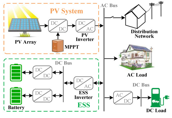
Figure 1.
Structure of master–slave-organized islanded microgrid.
In addition, ESS not only stabilizes the AC bus voltage, but also takes on the function of energy storage. The power generated by PV array varies with the changes in the temperature and solar irradiance, so it is necessary to achieve energy balance in the islanded microgrid. In the system of Figure 1, if the power generated by the PV system is greater than the rated power of the load, the excess power will charge the battery in ESS. Conversely, PV array and ESS together provide power to the load.
In this paper, only the controller of the PV inverter is optimized to improve the output power quality of the PV system. For the control method of the ESS inverter, we use a double-loop PI controller to perform tracking control of the inverter output voltage to the reference voltage. The transformation angle of the ESS is provided by a voltage controlled oscillator (VCO) [12], and transformation angle of the PV system is obtained by the phase-locked-loop (PLL), which is phase-locked to the AC bus.
3. Dynamic Model of PV Inverter
In this section, according to Figure 2, the dynamic model of the PV system is established by using Kirchhoff’s law. Besides, the function of the controller is realized by pulse-width modulation (PWM) generator. The control signal is transmitted to PWM generator and generate six-phase pulse signal to control VSC. Due to the fact that the PV inverter is regarded as slave controller of master–slave-organized islanded microgrid, thus we need to establish a current-controlled mathematical model for PV inverter. The relationship between the three-phase voltage and current in -frame in PV system is shown as follows [26]
where vector , and are the space vectors of the three phase variables , and . and represent the resistance and inductance of R-L filter. Furthermore, the terminal voltage of PV inverter can be expressed as , where is the three-phase PWM modulating wave. So, Equation (1) can be rewritten as
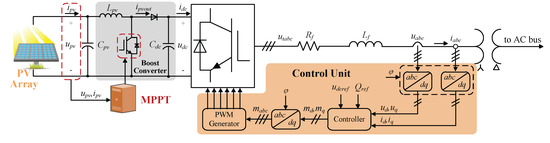
Figure 2.
Detailed structure and control loop of photovoltaic (PV) system.
Transform model (2) from -frame to -frame as [26]
where , , , , and are components of d and q axes of three-phase variables , and , respectively. According to reference [26], separating the d-axis and q-axis components of (3) as
where . In the DC side of PV system, the relationship between DC voltage and current , can be expressed as
where is the output current of boost circuit, is the DC side current of inverter, and is the DC-link capacitance.
In -frame, active power and reactive power in the system can be calculated as
Neglecting the power consumption of inverter and filter circuit, the active power equation between DC side and terminal side of PV system in -frame can be written as [27]
In conclusion, the current-controlled mathematical model of islanded PV system is summed up as follows
In model-based control, the control effect depends on the accuracy of model information. However, in the actual operation of the system, there are measurement errors in resistance , inductance , and capacitance . Therefore, the adaptive control is introduced to achieve online parameter identification. The adaptive parameters are defined as follows:
thus the mathematical model Equation (11) can be rewritten as
where , and are lumped disturbances of PV system, and will be observed by DO.
4. DFA-SMB Controller Design and Stability Analysis
In this section, a novel DFA-SMB controller is designed for PV inverter to enhance the anti-disturbance capability of the PV system and reduce the power chattering. The control goal is to stabilize the DC bus voltage and control the output power. The following is the design process of the controller. In the design process, represents the estimated value of the corresponding variable •, represents the estimated error defined as . Figure 3 illustrates the structure of designed DFA-SMB controller. Obviously, the whole controller is a double-loop control structure. The design of the controller is based on sliding mode backstepping control. Moreover, adaptive control and disturbance-observer are used to perform the adaptive estimation of model parameters and the observation of lumped disturbances respectively, which enhances the dynamic characteristics of the controller.
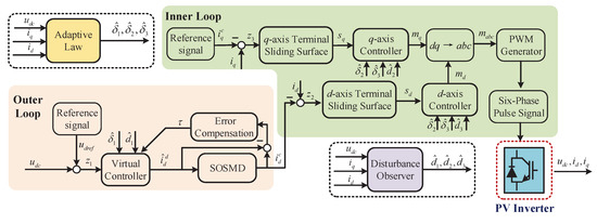
Figure 3.
Block diagram of disturbance finite-time adaptive sliding mode backstepping (DFA-SMB) controller for PV inverter.
4.1. Virtual Controller Design with Sosmd
Define the DC-link voltage tracking error as
where is DC-link reference voltage. Differentiating both side of Equation (14), we can get
To stabilize the Equation (15), we choose the Lyapunov function as , then, the derivative of can be calculated as
Then, according to Lyapunov asymptotic stability theory, the derivative of must satisfy the condition that it is negative definite. Therefore, considering the influence of adaptive control and DO, we choose the virtual controller from Equation (16) as
where is positive scalar. is the observation error boundary of disturbance and satisfies . is the adaptive law of , and , where and are positive constants. is defined in Equation (21). is the signum function represent as
According to Figure 3, the virtual controller is in the outer loop structure, and its output signal is used as a reference for the inner loop controller after passing through SOSMD.
In the design of the traditional backstepping controller, it is often necessary to use the derivative of the designed virtual controller. There will be a large number of differential processes affecting the control effect of the controller. As a result, SOSMD is introduced to replace the traditional command-filter in [18], which can eliminate the problem of differential expansion and guarantee the convergence of the filtering error in finite-time. The SOSMD is defined as [28]
where and are positive constants, is the virtual control law designed in Equation (17), and are estimated values of and .
Remark 1.
Choose proper parameters and , then the estimation error of SOSMD will converge in finite-time [28].
Define the error compensating signal by
where represents the output signal of the SOSMD.
Redefine the error as
Taking into account Equations (14), (17) and (20), the derivative of is calculated as
where is defined in Equation (25).
To stabilize error , the Lyapunov candidate function is selected as , and then the derivative of can be calculated as
and the adaptive law of is selected as
where represents the projection operator(see in the Appendix A) which guarantee the bounds of parameters estimation, is a positive scalar.
4.2. Controller Design with Terminal Sliding Mode Surfaces
Define the -frame current error
In order to further improve the robustness of the system, the terminal sliding mode control (TSMC) is introduced into the q-axis controller and d-axis inner loop controller. Define the terminal sliding mode surface
where and are the designed constant of sliding mode surface, , , and are the positive odd numbers which , .
Let us take as an example. Set , then can be rewritten as
when the system reaches the sliding surface, , Equation (27) can be calculated as
and the time that the system reaches the equilibrium point along the sliding surface can be calculated as [29]
The time for the system to move from any initial state to the sliding surface is defined as . Thus, the TSMC method can make the system converge from any initial state to the equilibrium point in finite-time . Similarly, the time required for the system to reach the equilibrium point along the sliding surface can be calculated.
In order to stabilize the whole system, the Lyapunov function is designed as
where (i = 2,3) represent adaptive gains.
Define and as terminal attractors. Then, combining Equations (23) and (30), the derivative of the Lyapunov function can be calculated as
Considering sliding mode reaching law
and the controllers and in -frame are designed as
where , , , are the designed positive constants. and are the observation error boundaries of disturbance and which satisfy , , , , where , , and are positive scalars. Furthermore, represents the saturation function defined as
where is the layer of the sliding surface.
Moreover, also according to Equation (32) and considering the boundedness of parameter estimation, the adaptive update laws of and are designed as
where , are positive scalars.
4.3. Design of the Disturbance-Observer
The initial DO is designed as
where is the observer gain vector. Substituting (37) into (39), we can get
In Equation (40), since the derivative of the state variable x cannot be directly measured, the process of derivation will amplify the noise of the state variable and affect the accuracy of interference estimation. Therefore, in this paper, the auxiliary variable is proposed to avoid the derivation of the state variable.
Define auxiliary variable , , thus Equation (40) can be rewritten as
Consequently, the improved DO for the PV inverter can be expressed as
The disturbance-observer in this paper is designed in continuous-time. By means of auxiliary variable , the improved DO can obtain the estimated disturbance value without calculating the derivative of the state variable x, so it is not necessary to design a filter link, in which the design process of the observer is simplified.
4.4. Stability Analysis
In order to consider the stability of DO, reselect Lyapunov candidate function as
Subsequently, the derivative of can be calculated as
Note that the term in Equation (45) has the following unequal relationship
Similarly
Furthermore, in order to eliminate the coupling term , define , then we can obtain
Assuming the condition can be satisfied, then inequality Equation (48) can be represented as
Evidently, this condition can be achieved by adjusting the parameter .
Subsequently, substituting Equations (42), (46), (47) and (49) into (45), and according to the definition of saturation function, we obtain
Through Young’s inequality, has the following unequal relationship
Similarly, has the following unequal relationship
Based on the literature [28], the filtering error of SOSMD is bounded in finite-time, thus compensated tracking error is bounded, indicating that all the signals in the control system can be regarded as semi-globally uniformly ultimately bounded.
5. Results and Analysis
In this section, based on Figure 1, a 100 kW master–slave-organized islanded PV microgrid was established in MATLAB/Simulink to verify the accuracy of the designed DFA-SMB controller. The parameters of the PV system and DFA-SMB controller are summarized in Table 1 and Table 2. There are many parameters generated in the design of the DFA-SMB controller. In the simulation, we have debugged all the parameters to achieve the best control effect. Firstly, we remove the DO and parameter adaptive control in the controller, and set the sliding mode parameters and to 0. Then adjust the parameters , and to make the system reach a relatively satisfactory state. Subsequently, adjust the sliding mode parameters , to make the system robust when a disturbance occurs. Finally, the adaptive and DO parameters are adjusted to reduce the chattering and tracking errors of the system.

Table 1.
The basic parameters of PV system.
Table 2.
Parameters of DFA-SMB controller.
The entire simulation process lasts 2 s. The controller starts at t = 0.05 s. When t = 0.4 s, the incremental conductance maximum power point tracking (MPPT) controller intervenes, and the PV system reaches the maximum power point. In addition, the influence of load variation on a PV inverter in islanded microgrid has been studied. When t = 1.65 s, the three-phase balanced load accessed to the system changes from 63 kW to 115 kW. When t = 1.8 s, three-phase six-pulse nonlinear diode-bridge accessed to simulate the non-linear load, and the total load power reaches 134 kW.
Figure 4 shows the curves of irradiance and temperature in the simulation. The output power of the PV array decreases as the irradiance drops or the temperature rises. When the temperature is 25 and the irradiance is 1000 , the output power of the PV array reaches the rated value of 100 kW.
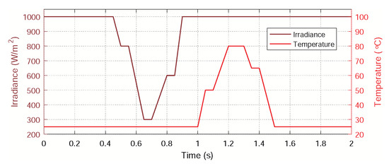
Figure 4.
The curves of irradiance and temperature.
In order to fully verify the advancement of DFA-SMB controller, the designed controller is compared to finite-time adaptive command-filtered backstepping (FACB), command-filtered backstepping (CB) [18], and PI controllers in the simulation. Figure 5 shows the DC bus voltage of the PV system using different controllers, with set to 500 V. Comparing the voltage tracking performance of the other three strategies, the proposed DFA-SMB scheme can track the DC-link voltage stably, with fast convergence rate and less steady-state error. Especially, with changing the irradiance, temperature and load change, the proposed control ensures that the voltage fluctuates within a small range. However, in the same case, the DC voltage under PI control has the largest deviation from the reference value. Because of the introduction of adaptive TSMC, the control effect under DFA-SMB and FACB scheme is better than that under CB and PI, indicating that after considering adaptive TSMC in CB, the effect of disturbance on DC voltage is restrained and the robustness of the system is improved. Moreover, by comparing the control effects of DFA-SMB and FACB controllers, the role of DO in the controller is verified. The lumped disturbances of PV the system observed by DO are shown in Figure 6. The proposed DO can observe the disturbances and provide estimated disturbance information to the controller, improving the anti-disturbance ability of the system. Moreover, if there are no disturbances in the system, the DO observation values are also approximately equal to the unknown part of the dynamic model. A comparison of the control effect between DFA-SMB and FACB controller indicates that the DO in the DFA-SMB controller can further reduce the tracking error when a disturbance occurs, and the impulse generated during the load variation can also be restrained. Consequently, the DFA-SMB controller is superior to the other three controllers in the DC voltage control and has better dynamic characteristics and robustness in the presence of disturbances.
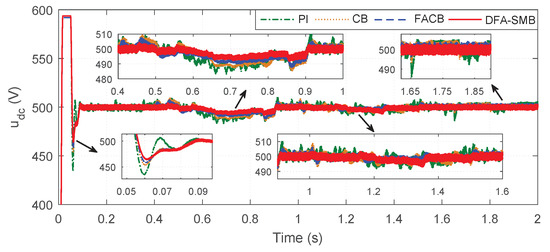
Figure 5.
Tracking performance of DC voltage under different controllers.
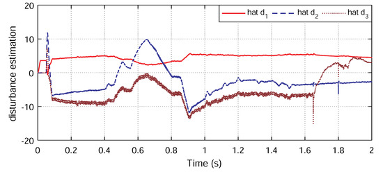
Figure 6.
Lumped disturbances observed by disturbance-observer (DO).
The same conclusion can be drawn from Figure 7, indicating the output active power comparison of the PV system under different controllers. The chattering problem of the active power curve is the most serious under PI control, and there is a large fluctuation during load variation at 1.65 s and 1.8 s. In contrast, the active power curves controlled by CB and FACB controllers are relatively smooth, but they are still sensitive to external disturbances. In addition, by observing lumped disturbances with DO, the fluctuation in the output active power is further reduced, and the impact of load variation on the output power is significantly suppressed.
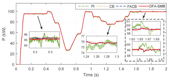
Figure 7.
Active power curves under different controllers.
Figure 8 illustrates the estimated values of the adaptive parameters designed in Equation (12). It can be seen that the estimated values of the parameters fluctuate near the actual value when the system runs. The adaptive control can adjust the system parameters appropriately to improve the control effect in face of system parameter disturbances. Thus, the adaptive estimation is not only an identification of the parameter values, but also allows the system to better cope with external interference in a dynamic and robust manner. Figure 9a shows the input and output signal of the SOSMD, where it can be seen that the output signal is basically consistent with the input signal. It means that the SOSMD works in a stable state. Figure 9b depicts the compensation signal curve of the SOSMD.
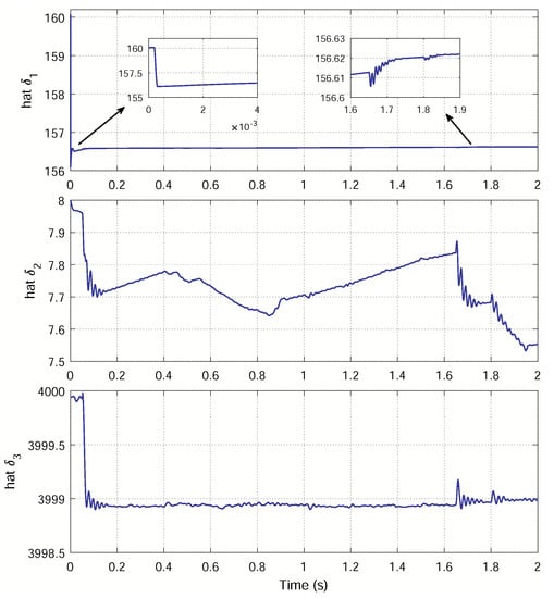
Figure 8.
Adaptive estimation of system parameters.
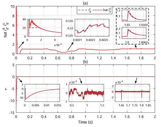
Figure 9.
(a) Input and output signals of second-order sliding mode differentiator (SOSMD). (b) Compensation signal of SOSMD.
In the simulation, the reference value of q-axis is set to 0, that is to say, we want the output reactive power of the PV system to be 0. Phase-contrast between the output voltage and current in the PV system under the DFA-SMB controller is shown in Figure 10a. This shows that the DFA-SMB controller is also effective in reactive power control. Figure 10b shows the output three-phase current of the PV system under the DFA-SMB controller. The output current of the PV system changes steadily when solar irradiance and temperature change, and the output power is changed by varying the current. Therefore, the quality of the output power depends on the output current. In Figure 11, we compare the total harmonic distortion (THD) of the output current controlled by different controllers when the system is stable. It is worth noting that the THD of PV system output current under DFA-SMB scheme is , while it is under PI control, under CB control and under FACB. We concluded that DFA-SMB also has excellent control performance in steady-state, meeting the requirement of power quality. Furthermore, Figure 12 shows the three-phase current curve in the presence of load variations under the DFA-SMB controller. The system is disturbed due to load transformation at 1.65 s and 1.8 s, while the output current under DFA-SMB controller has little distortion when a disturbance occurs and can quickly return to stability, thus further verifying the dynamic performance and robustness of the DFA-SMB controller.
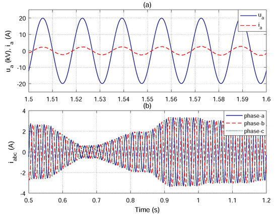
Figure 10.
(a) Phase contrast between output voltage and current in PV system under DFA-SMB controller at t = 1.5–1.6 s. (b) Output three-phase current of PV system under DFA-SMB controller at t = 0.5–1.2 s.
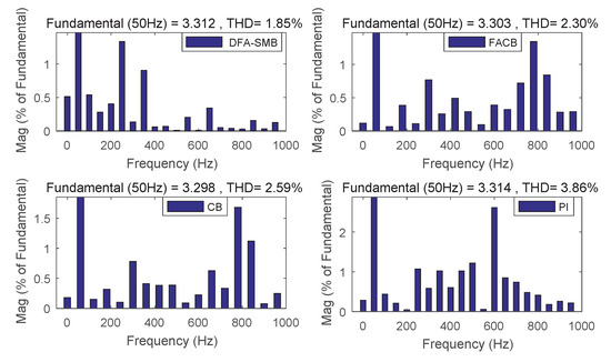
Figure 11.
Total harmonic distortion (THD) analysis of PV system output current under different controllers.
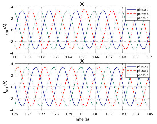
Figure 12.
Current waveform of PV system during load conversion under DFA-SMB controller.
6. Conclusions
In this paper, a novel DFA-SMB controller for PV inverter in master–slave-organized islanded microgrid has been successfully developed to enhance the anti-disturbance capability of the PV system and reduce the power chattering. The DFA-SMB control strategy is based on a backstepping control strategy. Moreover, the SOSMD, adaptive parameter estimation method, TSMC and DO are integrated in the controller, reducing the amount of calculations of the controller and improving the anti-disturbance performance. In MATLAB/Simulink, a 100 kW PV system has been established in a master–slave-organized islanded microgrid, and the control effects between DFA-SMB and FACB, CB, PI for PV inverter are compared. The results show that the DC voltage is more stable, and the active power curve is smoother using the DFA-SMB controller. In the presence of disturbance, the DFA-SMB controller can also minimize the effect of the disturbance on the system as much as possible. Therefore, DFA-SMB is verified to have better static, dynamic characteristics and robustness than the other three controllers. Future investigation will be focused on two goals: (i) to build an experimental platform to verify the effectiveness of the proposed controller; (ii) based on the DFA-SMB controller, investigate the fixed-time control of the system and the cooperative control strategy of a multi-PV system and multi-energy storage system.
Author Contributions
Conceptualization: C.Y.; writing—original draft: S.N. and Y.D.; funding acquisition: X.H. and D.Z.; validation: Y.D.; methodology: C.Y. and S.N. All authors have read and agreed to the published version of the manuscript.
Funding
This work was partially supported by the National Natural Science Foundation of Jiangsu Province (BK20181021), the Open Research Fund of Jiangsu Collaborative Innovation Center for Smart Distribution Network(XTCX201902), Industry-University-Research Cooperation Project of Jiangsu Province (BY2019023) and Scientific research fund project of Nanjing Institute of Technology (JCYJ201817).
Conflicts of Interest
The authors declare no conflict of interest.
Appendix A
In this paper, the role of the discontinuous projection operator [30] is to prevent the excessive estimation of the parameters in the DFA-SMB controller in PV system, thus ensuring the boundedness of the adaptive parameter estimation. We define the equation , where is the actual value of the estimated parameter, and are the adaptive estimation of the parameter and estimation error, respectively. The adaptive law with the discontinuous projection operator is designed as:
where is a designed positive constant, and f is the designed adaptive function. Furthermore, we can define the function of discontinuous projection operator as:
where represents the upper limit of the estimated value of . The projection operator for any adaptive function f has the following conclusions [30]:
A.1.
A.2.
References
- Zhou, X.; Wang, J.; Ma, Y. Linear active disturbance rejection control of grid-connected photovoltaic inverter based on deviation control principle. Energies 2020, 13, 3790. [Google Scholar] [CrossRef]
- Wu, Y.; Lin, H. Standards and guidelines for grid-connected photovoltaic generation systems: A review and comparison. IEEE Trans. Ind. Appl. 2017, 53, 3205–3216. [Google Scholar] [CrossRef]
- Rahmani, R.; Moser, I.; Seyedmahmoudian, M. Multi-agent based operational cost and inconvenience optimization of PV-based microgrid. Solar Energy 2017, 150, 177–191. [Google Scholar] [CrossRef]
- Li, J.; Li, Y.; Wu, L. Optimal operation for community-based multi-party microgrid in grid-connected and islanded modes. IEEE Trans. Smart Grid 2018, 9, 756–765. [Google Scholar] [CrossRef]
- Ma, L.; Xu, G. Distributed resilient voltage and reactive power control for islanded microgrids under false data injection attacks. Energies 2020, 13, 3828. [Google Scholar] [CrossRef]
- Zeng, Z.; Shao, W. Reconnection of micro-grid from islanded mode to grid-connected mode used sliding Goertzel transform based filter. IET Renew. Power Gener. 2017, 11, 1041–1048. [Google Scholar] [CrossRef]
- Damavandi, M.Y.; Neyestani, N.; Chicco, G.; Shafie-khah, M.; Catalão, J.P.S. Aggregation of distributed energy resources under the concept of multienergy players in local energy systems. IEEE Trans. Sustain. Energy 2017, 8, 1679–1693. [Google Scholar] [CrossRef]
- Díaz, N.L.; Guarnizo, J.G.; Mellado, M.; Vasquez, J.C.; Guerrero, J.M. A robot-soccer-coordination inspired control architecture applied to islanded microgrids. IEEE Trans. Power Electron. 2016, 32, 2728–2742. [Google Scholar] [CrossRef]
- Lou, G.; Gu, W.; Wang, L.; Xu, B.; Wu, M.; Sheng, W. Decentralised secondary voltage and frequency control scheme for islanded microgrid based on adaptive state estimator. IET Gener. Transm. Distrib. 2017, 11, 3683–3693. [Google Scholar] [CrossRef]
- Gholami, S.; Aldeen, M.; Saha, S. Control strategy for dispatchable distributed energy resources in islanded microgrids. IEEE Trans. Power Syst. 2018, 33, 141–152. [Google Scholar] [CrossRef]
- Delghavi, M.B.; Yazdani, A. Sliding-mode control of AC voltages and currents of dispatchable distributed energy resources in master-slaveorganized inverter-based microgrids. IEEE Trans. Smart Grid 2019, 10, 980–991. [Google Scholar] [CrossRef]
- Delghavi, M.B.; Shoja-Majidabad, S.; Yazdani, A. Fractional-order sliding-mode control of islanded distributed energy resource systems. IEEE Trans. Sustain. Energy 2016, 7, 1482–1491. [Google Scholar] [CrossRef]
- Mahmood, H.; Michaelson, D.; Jiang, J. Strategies for independent deployment and autonomous control of PV and battery units in islanded microgrids. IEEE J. Emerg. Sel. Top. Power Electron. 2015, 3, 742–755. [Google Scholar] [CrossRef]
- Sachs, J.; Sawodny, O. A two-stage model predictive control strategy for economic diesel-PV-battery island microgrid pperation in rural areas. IEEE Trans. Sustain. Energy 2016, 7, 903–913. [Google Scholar] [CrossRef]
- Mathew, P.; Madichetty, S.; Mishra, S. A multi-level control and optimization scheme for islanded PV based microgrid: A control frame work. IEEE J. Photovolt. 2019, 9, 822–831. [Google Scholar] [CrossRef]
- Arsalan, M.; Iftikhar, R.; Ahmad, I.; Hasan, A.; Sabahat, K.; Javeria, A. MPPT for photovoltaic system using nonlinear backstepping controller with integral action. Sol. Energy 2018, 170, 192–200. [Google Scholar] [CrossRef]
- Roy, T.K.; Mahmud, M.A. Active power control of three-phase grid-connected solar PV systems using a robust nonlinear adaptive backstepping approach. Sol. Energy 2017, 153, 64–76. [Google Scholar] [CrossRef]
- Farrell, J.A.; Polycarpou, M.; Sharma, M.; Dong, W. Command filtered backstepping. IEEE Trans. Autom. Control 2009, 54, 1391–1395. [Google Scholar] [CrossRef]
- Du, W.; Yang, G.; Pan, C.; Xi, P.; Chen, Y. A sliding-mode-based duty ratio controller for multiple parallelly-connected DC–DC converters with constant power loads on MVDC shipboard power systems. Energies 2020, 13, 3888. [Google Scholar] [CrossRef]
- Cucuzzella, M.; Incremona, G.P.; Ferrara, A. Design of Robust Higher Order Sliding Mode Control for Microgrids. IEEE Trans. Autom. Sci. Eng. 2015, 5, 393–401. [Google Scholar] [CrossRef]
- Xu, D.; Zhang, W.; Jiang, B.; Shi, P.; Wang, S. Directed-graph-observer-based model-free cooperative sliding mode control for distributed energy storage systems in DC microgrid. IEEE Trans. Ind. Inform. 2020, 16, 1224–1235. [Google Scholar] [CrossRef]
- Pradhan, S.; Singh, B.; Panigrahi, B.K.; Murshid, S. A composite sliding mode controller for wind power extraction in remotely located solar. IEEE Trans. Ind. Electron. 2019, 66, 5321–5331. [Google Scholar] [CrossRef]
- Zhu, Y.; Fei, J. Adaptive global fast terminal sliding mode control of grid-connected photovoltaic system using fuzzy neural network approach. IEEE Access 2017, 5, 9476–9484. [Google Scholar] [CrossRef]
- Zhang, J.; Liu, X.; Xia, Y.; Zuo, Z.; Wang, Y. Disturbance observer-based integral sliding-mode control for systems with mismatched disturbances. IEEE Trans. Ind. Electron. 2016, 63, 7040–7048. [Google Scholar] [CrossRef]
- Huang, J.; Ri, S.; Fukuda, T.; Wang, Y. A disturbance observer based sliding mode control for a class of underactuated robotic system with mismatched uncertainties. IEEE Trans. Autom. Control 2019, 64, 2480–2487. [Google Scholar] [CrossRef]
- Delghavi, M.B.; Yazdani, A. Islanded-mode control of electronically coupled distributed-resource units under unbalanced and nonlinear load conditions. IEEE Trans. Power Deliv. 2011, 26, 661–673. [Google Scholar] [CrossRef]
- Ajami, A.; Shotorbani, A.M.; Aagababa, M.P. Application of the direct Lyapunov method for robust finite-time power flow control with a unified power flow controller. IET Gener. Transm. Distrib. 2012, 6, 822–830. [Google Scholar] [CrossRef]
- Levant, A. Higher-order sliding modes, differentiation and outputfeedback control. Int. J. Control 2003, 76, 924–941. [Google Scholar] [CrossRef]
- Zheng, X.M.; Li, L.; Zheng, J.F.; Feng, Y. Non-singular terminal sliding mode backstepping control for the uncertain chaotic systems. In Proceedings of the 2008 2nd International Symposium on Systems and Control in Aerospace and Astronautics, Shenzhen, China, 10–12 December 2008. [Google Scholar] [CrossRef]
- Cai, Z.; De Queiroz, M.S.; Dawson, D.M. A sufficiently smooth projection operator. IEE Proc. Control Theory Appl. 2006, 51, 135–139. [Google Scholar] [CrossRef]


© 2020 by the authors. Licensee MDPI, Basel, Switzerland. This article is an open access article distributed under the terms and conditions of the Creative Commons Attribution (CC BY) license (http://creativecommons.org/licenses/by/4.0/).