Sustainable Protected Cropping: A Case Study of Seasonal Impacts on Greenhouse Energy Consumption during Capsicum Production

 ,
, 
 and
and 
Abstract

1. Introduction
- (1)
- Understand daily energy consumption during the crop cycle, identifying key factors (e.g., peak daily energy consumption, average energy consumption, etc.);
- (2)
- Analyse energy consumption and yield data with climate conditions using key variables, particularly specific temperature ranges within and outside of the high-tech greenhouse facility, as the basis for improving current sustainable practices in protected cropping in Australia;
- (3)
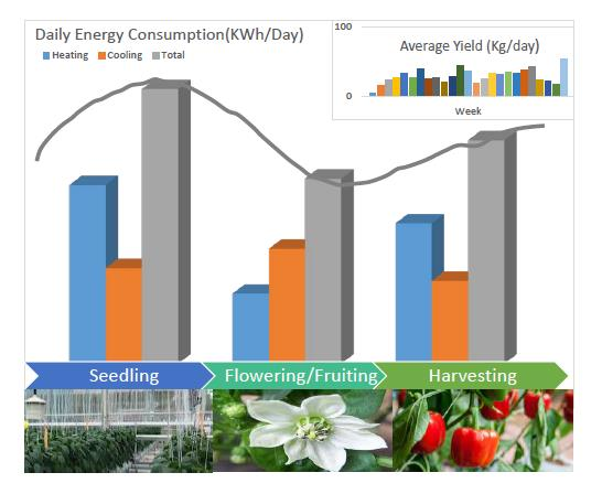
- Compare energy consumption over three different stages of the crop production (seedling, flowering/fruiting, and harvesting) and three seasons (spring, summer and autumn) lifecycle as the basis for developing guidelines and strategies for sustainable protected cropping;
- (4)
- Compare daily cooling, heating and total energy consumption over associated periods, predominantly identified as cooling, heating and mixed cooling/heating seasons, respectively.
2. Research Methodology
2.1. Baseline Model
2.2. Data Collection
3. Data Analysis and Results
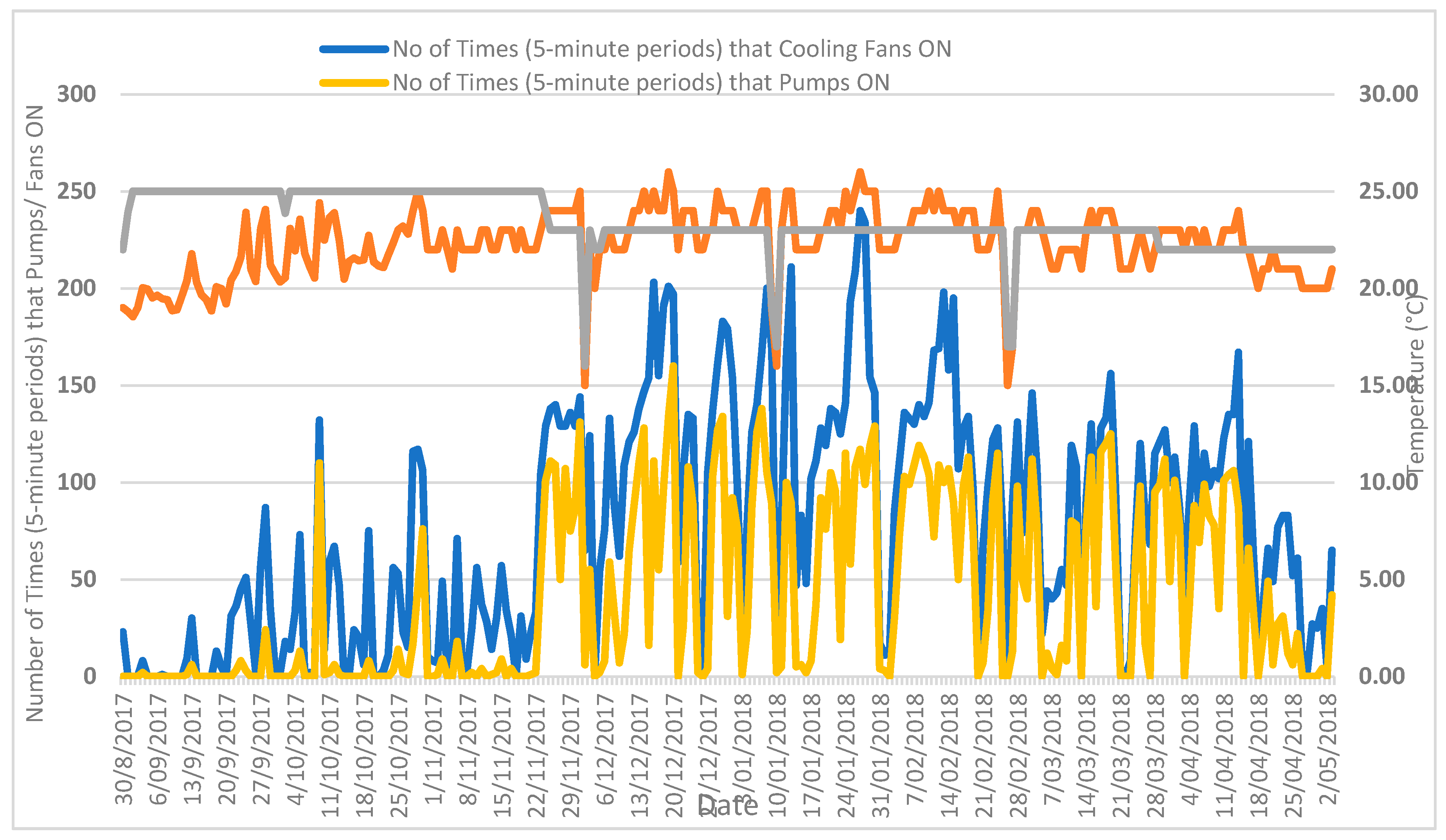
3.1. Analysis of Cooling, Heating, Power Consumption and Yield Data
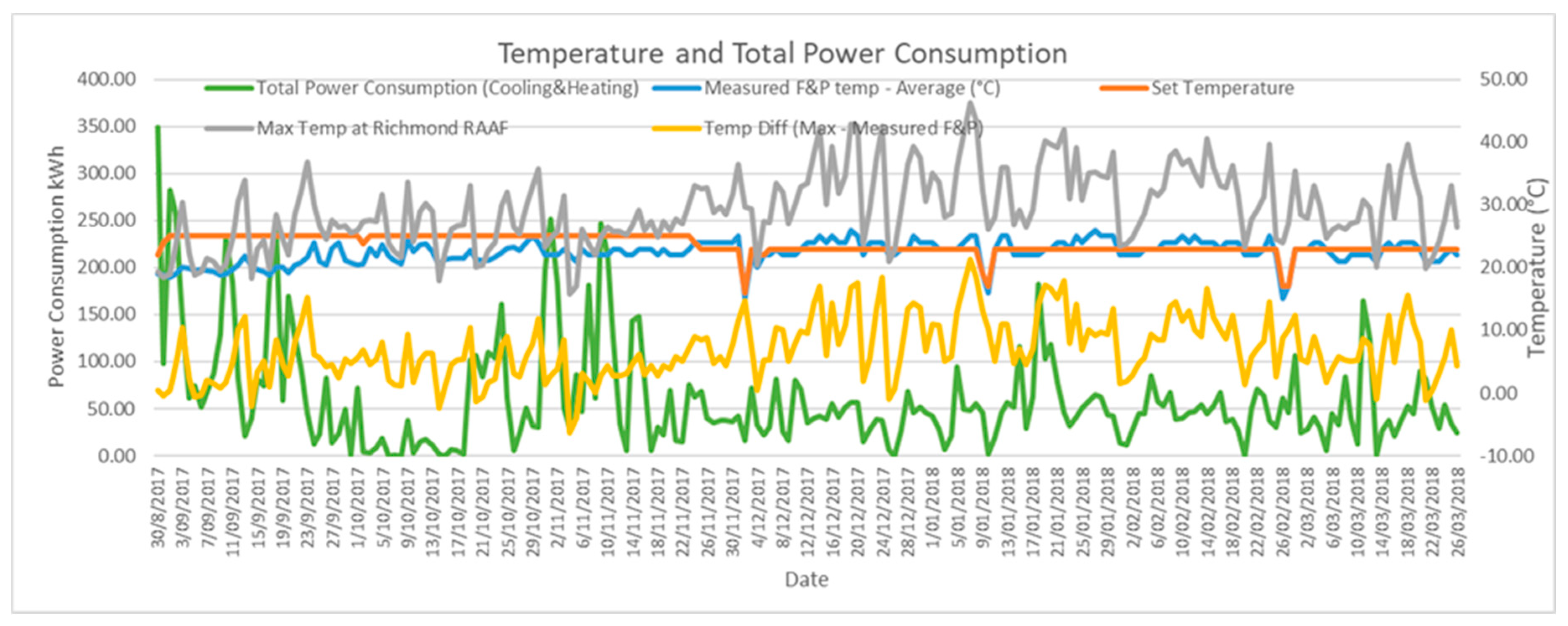
3.2. Overview of Temperatures and Power Consumption of a Greenhouse Capsicum Crop Cycle
3.3. Analysis of Energy Cost Based on Plant Growth Stages
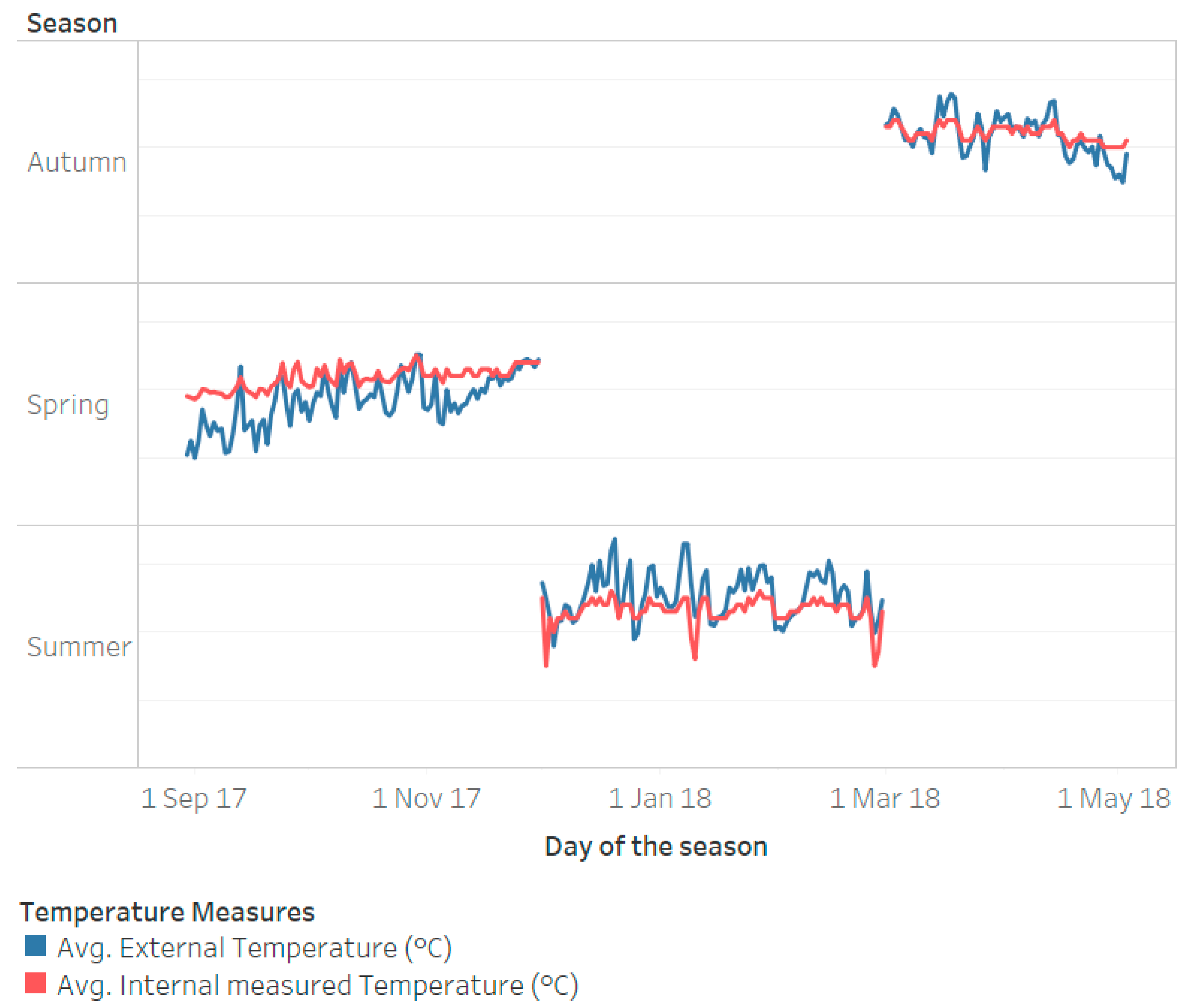
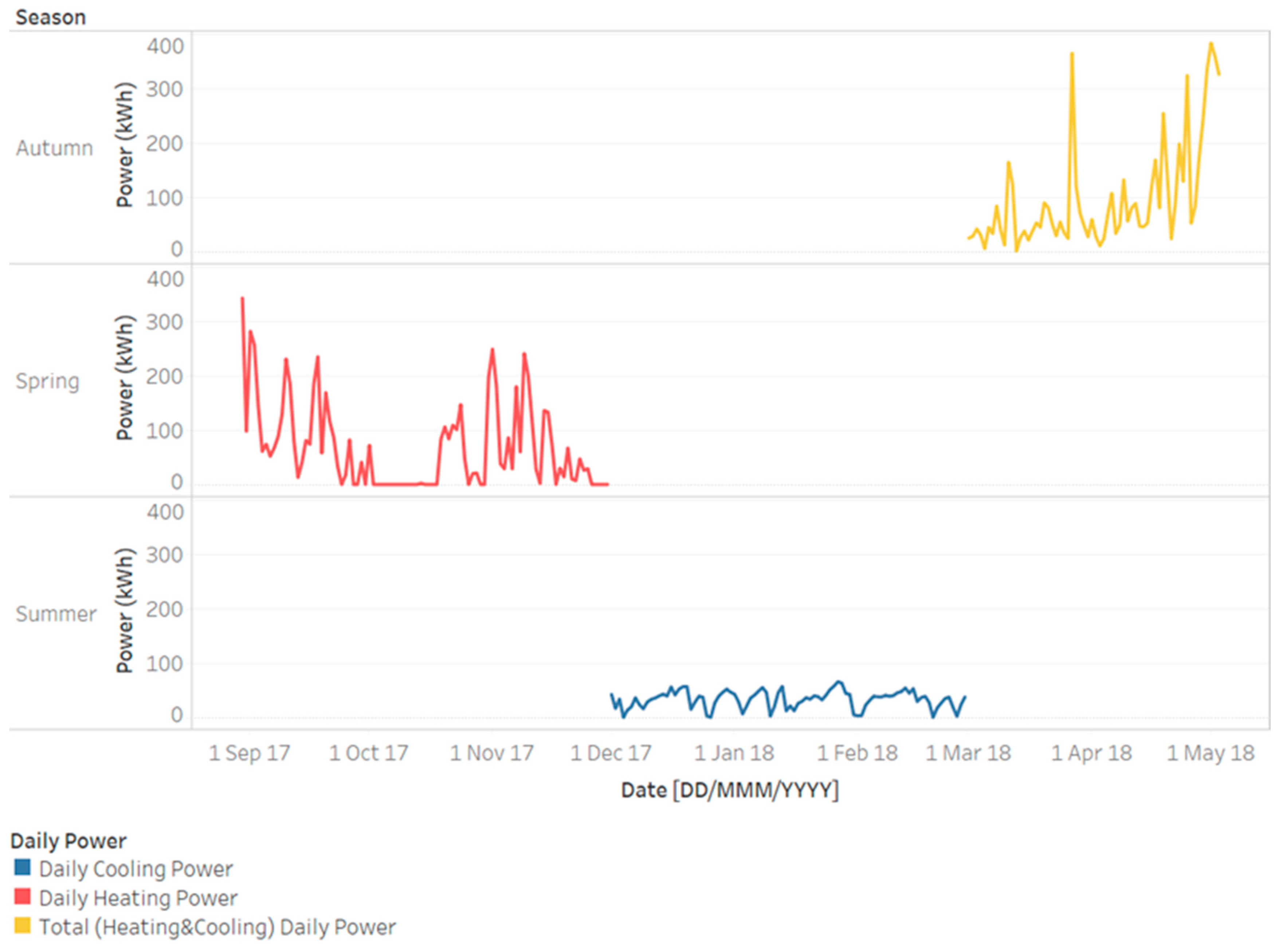
3.4. Analysis of Energy Cost Based on Seasons
3.5. Analysis of Cooling, Heating and Total Energy Consumption Cross Seasons for Crop Management Decision Making
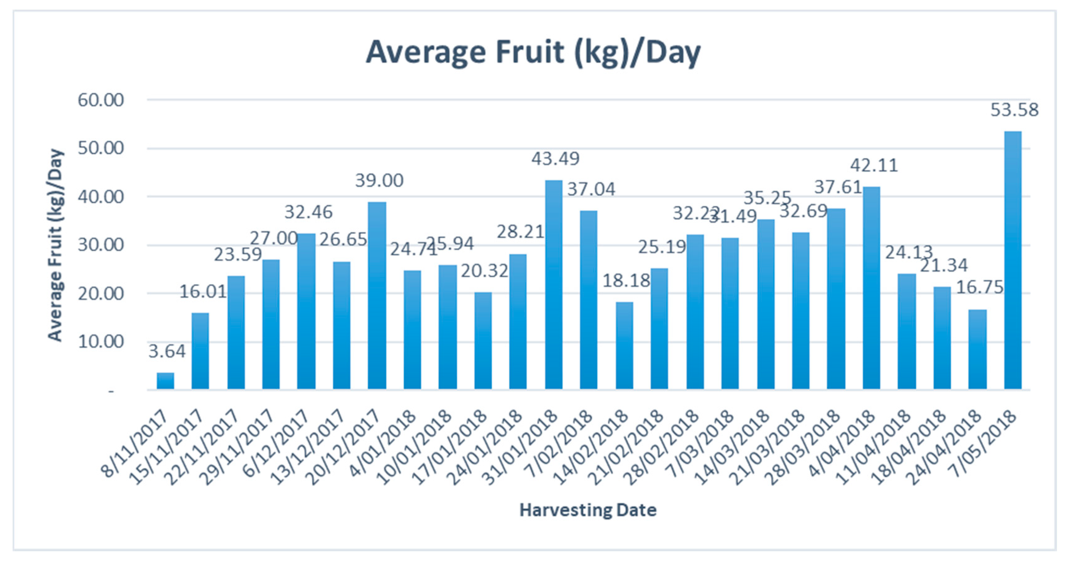
3.6. Analysis of Crop Production
4. Discussion
5. Conclusions
Author Contributions
Funding
Acknowledgments
Conflicts of Interest
Appendix A. Key Variables, Descriptive Statistics, and Correlation and Regression Analyses

| Variable | Unit of Measure | Description | Details |
|---|---|---|---|
| Fan and pump (F&P) active | Active or Non-active | Fan and Pump–ON/OFF | Water is circulated if required. Involves multiple stages. Variable F&P is a binary variable. Record of 1 means both fan and pump are ON. |
| Cooling active | Active or Non-active | Fan is ON/OFF | This is a binary variable. Record of 1 means fan is ON. |
| Meas F&P temp | Celsius (°C) | Measured F&P temperature | This is the measured temperature in the facility, also recorded under environmental measures. |
| Temp F&P active | Celsius (°C) | Temperature setting to activate cooling. | This temperature setting is changed as crop matures. This could be based on advice from growers. |
| Variable | Unit of Measure | Variable Description |
|---|---|---|
| Meas heat t | Celsius (°C) | The calculated value determined by Priva based on the user settings and other influences that have been included. |
| Meas return 1 (Wall) | Celsius (°C) | The measured water temperature on the return line of the heating pipes (at exit) on the wall. This measurement point is immediately prior to exiting the room |
| Meas wt 1 (Wall) | Celsius (°C) | The measured water temperature on the supply line of the heating pipes (at entry) on the wall. This measurement point is just at the entry of wall system to the room (same location as the exit point in the room) |
| Meas return 2 (Floor) | Celsius (°C) | The measured water temperature on the return line of the heating pipes (at exit) on the floor. This measurement point is just before the exiting the room |
| Meas wt 2 (Floor) | Celsius (°C) | The measured water temperature on the supply line of the heating pipes (at entry) on the floor. This measurement point is just at the entry of floor system to the room (same location as the exit point in the room) |
| Wall (system 1) total (KWH) | KWH | The cumulative total kWh consumption for the day of the wall heating. |
| Floor (system 2) total (KWH) | KWH | The cumulative total kWh consumption for the day of the floor heating. |
| Key Descriptive Statistics | Seedling | Flowers/Fruits | Harvesting |
|---|---|---|---|
| Mean | 3.68 | 8.54 | 26.79 |
| Standard Deviation | 5.59 | 10.35 | 16.12 |
| Range | 22.85 | 38.04 | 65.36 |
| Minimum | 0 | 0 | 0 |
| Maximum | 22.85 | 38.04 | 65.36 |
| Sum | 117.65 | 324.42 | 4741.73 |
| Count (No of days) | 32 | 38 | 177 |
| Measured F&P Temp-Average (°C) | Temp Diff (Max-Measured F&P Temp) | Total Cooling Power Consumption by Fan and Pump | Total Heating Power Consumption by Wall and Floor | Total Power Consumption (Cooling and Heating) | |
|---|---|---|---|---|---|
| Measured F&P temp-Average (°C) | 1.00 | ||||
| Temp Diff (Max-Measured F&P Temp) | 0.48 | 1.00 | |||
| Total cooling power consumption by Fan & Pump | 0.73 | 0.76 | 1.00 | ||
| Total Heating Power Consumption by Wall and Floor | −0.49 | −0.28 | −0.39 | 1.00 | |
| Total Power Consumption (Cooling and Heating) | −0.35 | −0.12 | −0.18 | 0.98 | 1.00 |
| Key Descriptive Statistics | Daily Power Consumption (Cooling)-kWh | Daily Power Consumption (Heating)-kWh |
|---|---|---|
| Mean | 3.68 | 103.78 |
| Standard Deviation | 5.59 | 89.71 |
| Range | 22.85 | 343.00 |
| Minimum | 0 | 0 |
| Maximum | 22.85 | 343.00 |
| Sum | 117.65 | 3321.00 |
| Temperature Differential | Definition |
|---|---|
| Diff A | Set temperature—Outside Average Temperature |
| Diff B | Maximum outside temperature—Set Temperature |
| Diff C | Measured temperature—Outside Average Temperature |
| Diff D | Maximum outside temperature—Measured Temperature |
| Diff E | Set temperature—Measured temperature |
| Diff F | Maximum outside temperature—Minimum outside temperature |
| Diff G | Measured temperature—Minimum outside temperature |
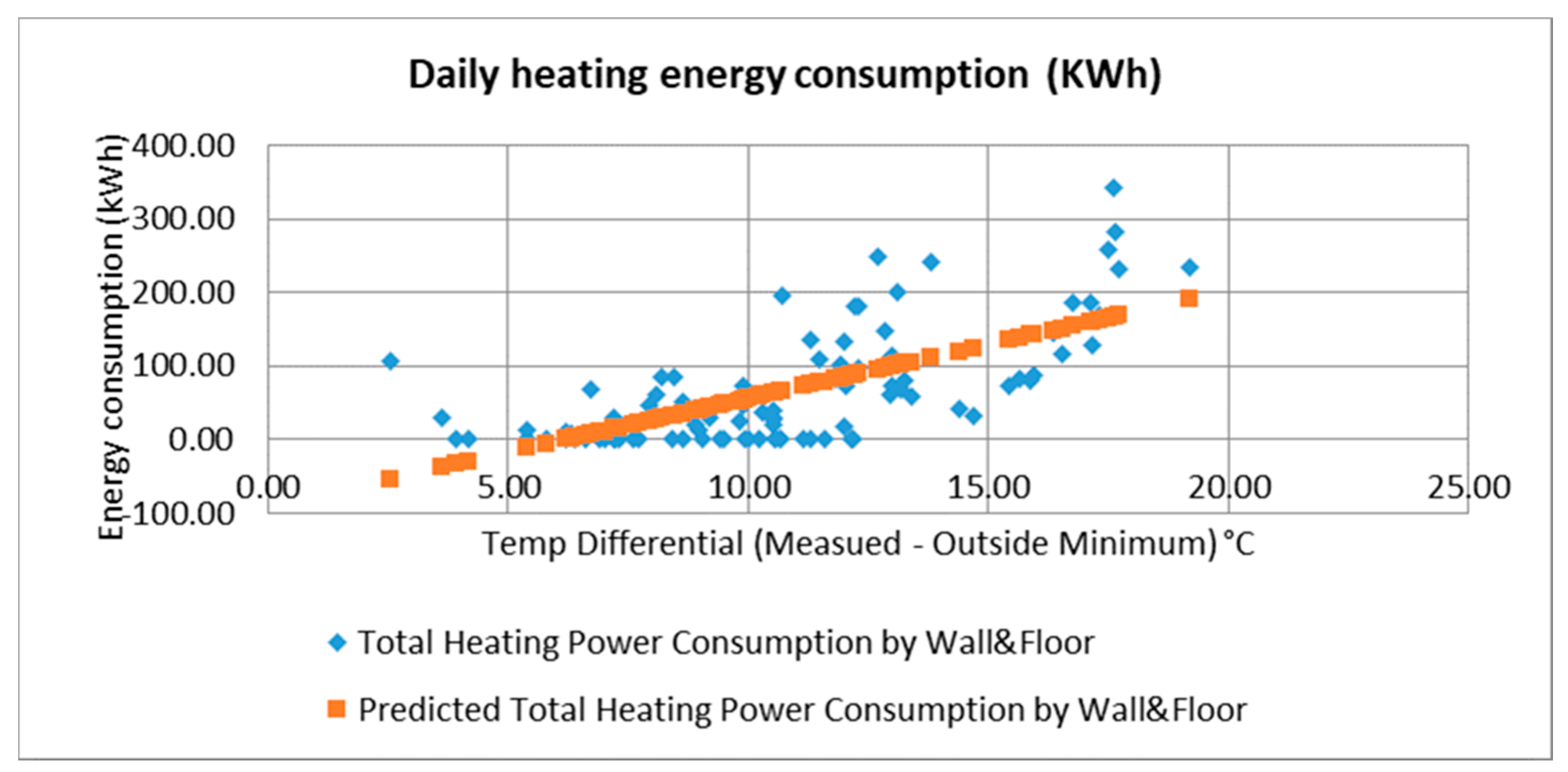
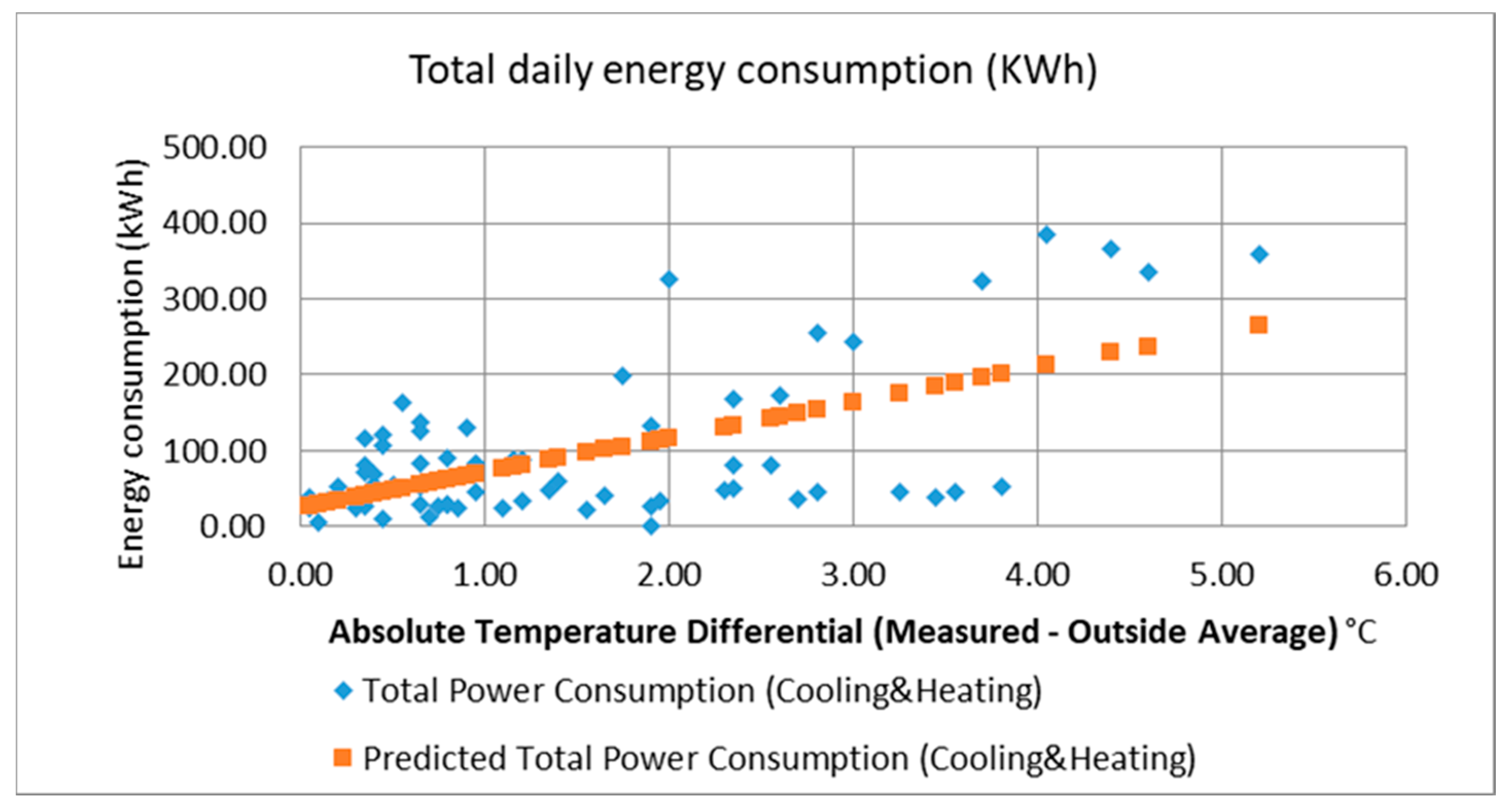
| Season/Main energy type | Temperature Differential | Daily Energy Consumption (KWh) | Regression Coefficients | Regression Equation |
|---|---|---|---|---|
| Spring/Heating | Measured-Min. Outside Temperature | Daily heating energy consumption | Multiple R: 0.68 R Square: 0.46 Intercept: −90.70 Gradient: 14.62 | Y = 14.62X − 90.70 |
| Summer/Cooling | Maximum Outside Temp-Measured | Daily cooling energy consumption | Multiple R: 0.67 R Square: 0.45 Intercept: 11.04 Gradient: 2.23 | Y = 2.23X + 11.04 |
| Autumn/Total energy | Measured-Outside Average Temp. | Daily total energy consumption | Multiple R: 0.61 R Square: 0.37 Intercept: 24.64 Gradient: 46.28 | Y = 46.28X +2 4.64 |
Appendix B. Details of Energy System Parameters, Measurement and Monitoring
- Combustion value of natural gas:
- ○
- Lower: 31.65 MJ/m3
- ○
- Upper: 35.17 MJ/m3
- The screen details used in the WSU greenhouse setup:
- ○
- Energy saving 45%
- ○
- Radiation limitation 50%
- ○
- Air exchange limitation 80%
- Energy saving based on the position of the screen:
- ○
- 1/8 at 70% screen cover
- ○
- 1/2 at 85% screen cover
- Specific capacity:
- ○
- 1.7 × (Pipe diameter [mm]/51) × (Number of pipes per cover/Roof width [m]). This is for round pipes only.
- ○
- Example 1 of the calculation of the Specific capacity:
- ○
- The pipe is round and has a diameter of 45 mm
- ○
- The cover width is 4 m
- ○
- There are 5 pipes per roof
- ○
- From the data above it appears that Formula 1 from the table above should be used. Completing the formula gives: Specific capacity = 1.7 × (45/51) × (5/4) = 1.9 W/(m2·°C)
- ○
- The formula above for the pipes gives us 2.1 W/(m2·°C) in compartments 1–9 for the floor pipes
- Specific area:
- ○
- Example of the calculation of the Specific area:
- ○
- The pipe is round and has a diameter of 51 mm (=0.051 m)
- ○
- The cover width is 3.2 m
- ○
- There are 4 pipes per roof
- ○
- From the formulas and data above the Specific area is determined as follows: Specific area = (4 × 0.051 × 100)/3.2) = 6.38%
- ○
- The number above is what is used in compartments 1–9 for the floor pipes
- The energy specifics of the air handling units (fan/heat exchanger unit) such as fan details as per WSU greenhouse settings:
- ○
- Fan motor: 1.8 kW
- ○
- Fan capacity: 4000 (m3/h)
- ○
- Pump capacity: 200 W
- ○
- Specific capacity: 33.7 W/(m2·°C)
- Those details were provided by ACIS during the commissioning of the job.
- Indication of the energy delivery/continuity coefficient of a spiral, expressed in Watts per m2 of spiral area (the area setting indicated above for each degree Celsius difference between the spiral and air that runs along the spiral).
- Different forms of energy are available for the different sources.
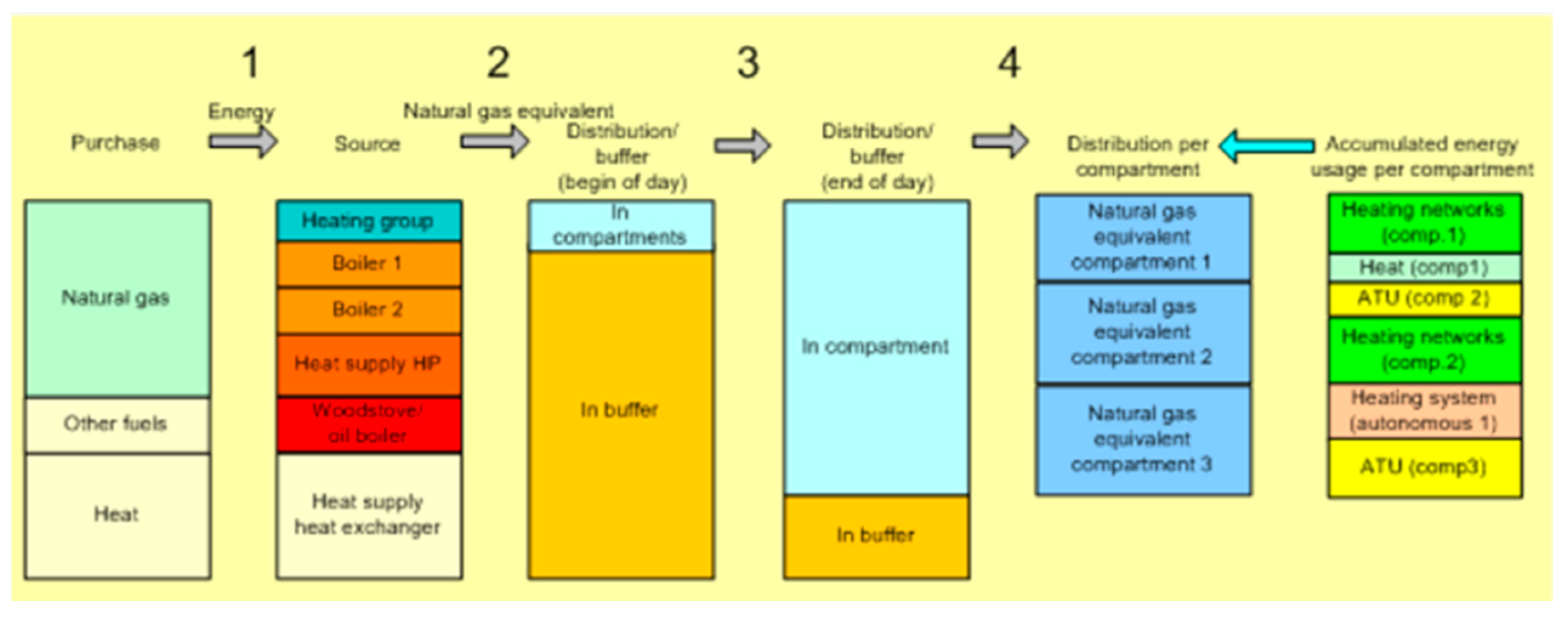
- The central sources such as the boiler, Heating Pump and the heat exchanger first supply the produced heat to the buffer (system dependent). The energy that arrives in the buffer from the start of the day onwards is converted into a gas equivalent using the natural gas equivalent conversion factor.
- 3.
- Emptying the buffer makes the heat available in the compartments. In this example, at the end of the day not all the purchased energy has been consumed in the compartments. A small fraction is still left in the buffer. Only the fraction of the energy that has actually been consumed in the compartments is allocated to the compartments.
- 4.
- For the distribution of the sum of the gas equivalents, the dealer must link the air treatment systems present to the corresponding compartment and any autonomous heating systems to the corresponding compartments.
- 5.
- Internally, the control determines per compartment the sum of the heat capacity of the heating networks (compartment and autonomous) and the air treatment systems. If an (autonomous) heating control or air treatment control is located in several compartments at the same time, the ratio of the heated surfaces and the compartment surfaces is decisive.
- 6.
- The total of the gas equivalents consumed over all compartments is distributed among the compartments. This distribution is based on the ratio of the heat capacity sums. In this way, transport losses are spread across the various compartments.

- 2 Max electricity network capacity
- Absolute max electricity import
- Max import from current clock hour.

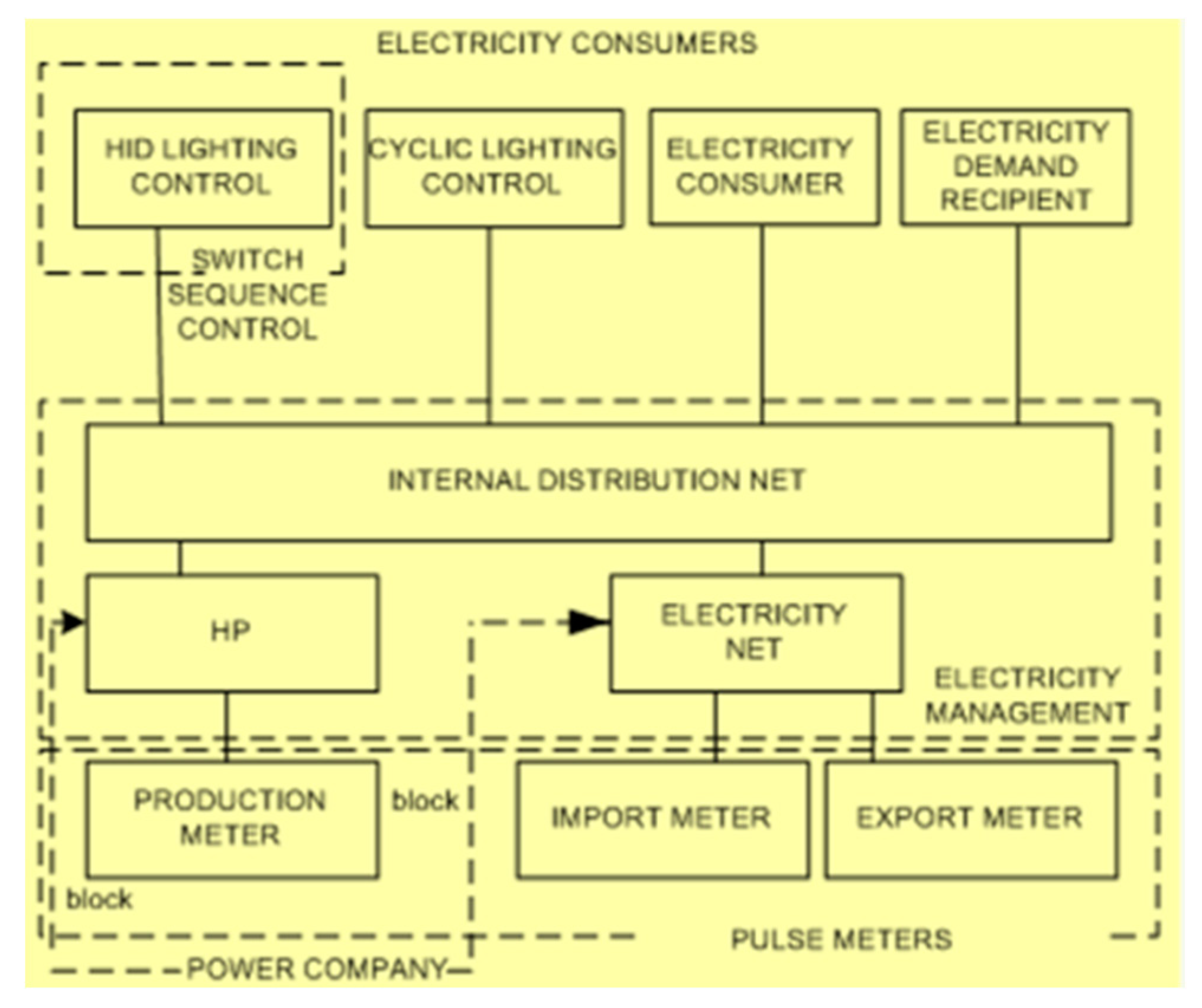
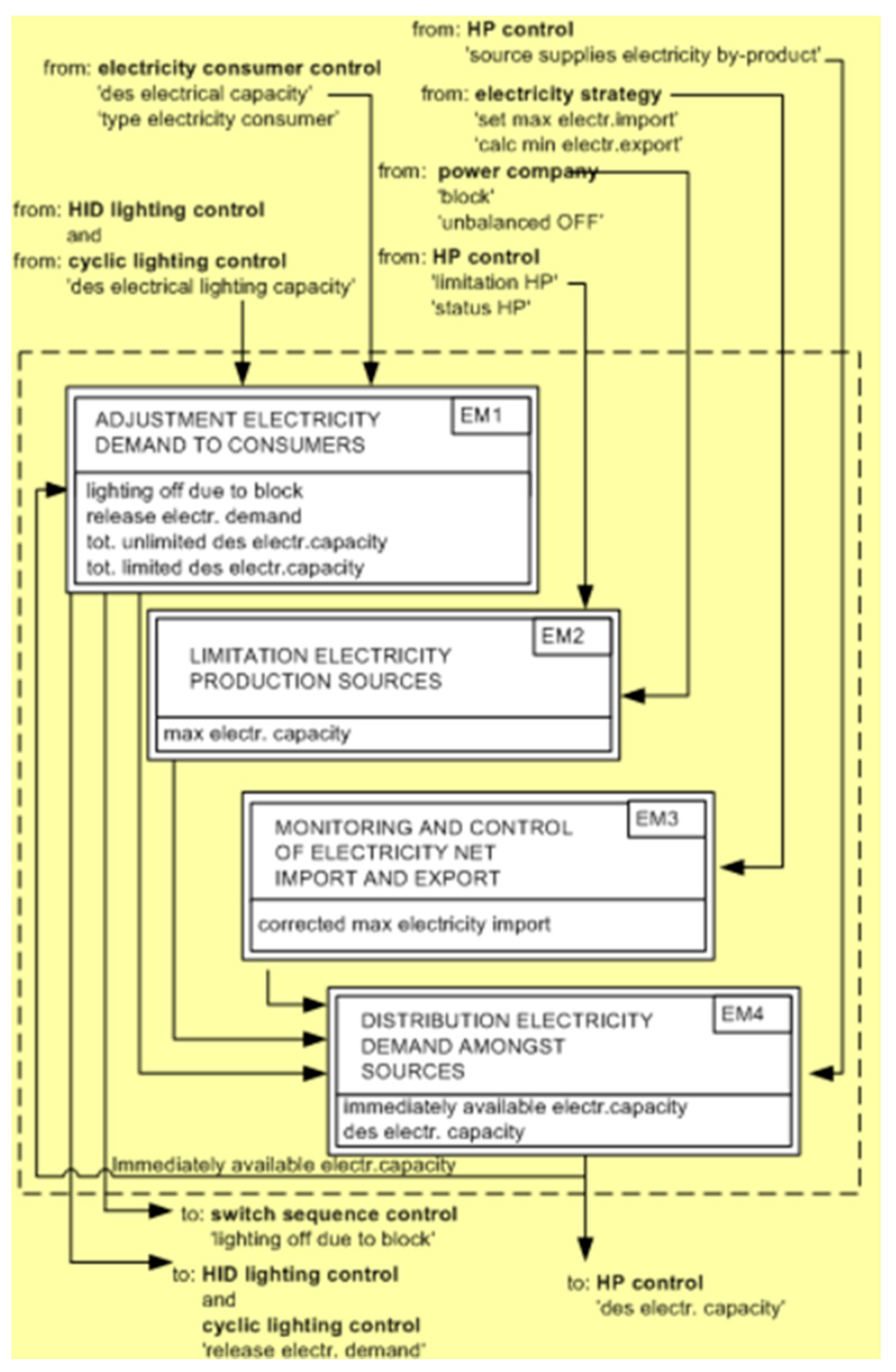
- Demands from the connected lighting systems (growing light and cyclic lighting, electricity consumers and recipients of electricity demand) are collected in module EM1-Adjustment electricity demand to consumers. In addition, the electrical capacity that is available immediately is used in conjunction with the set sequence numbers for electricity consumption by the various lighting systems and electricity consumers to determining which lighting systems may be switched on.
- The maximum electrical capacity is determined for each source in module EM2-Limitation electricity production sources. This also uses the block-out signal for the relevant source or a central ‘unbalanced OFF’ signal that can switch off one or more CHPs simultaneously. In the case of the CHP it also checks whether it is being limited by any other causes (Limitation CHP).
- If possible, the imported electrical capacity is readjusted in module EL3-Monitoring and controlling electricity network import and export, if the measured import capacity exceeds the set import limit. This module also ensures that an alarm is generated if the maximum import capacity is exceeded or if insufficient capacity is exported.
- The collected electricity demand is distributed across the available electricity sources in module EM4-Distribution electricity demand amongst sources. In so doing, the maximum capacity and the electricity by-product (for CHPs only) of the relevant sources are taken into account.
- Based on electricity demand, the CHP control switches on an CHP.

References
- Torrellas, M.; Antón, A.; Ruijs, M.; Victoria, N.G.; Stanghellini, C.; Montero, J.I. Environmental and economic assessment of protected crops in four European scenarios. J. Clean. Prod. 2012, 28, 45–55. [Google Scholar] [CrossRef]
- Zarei, M.J.; Navab, K.; Afshin, M. Life cycle environmental impacts of cucumber and tomato production in open-field and greenhouse. J. Saudi Soc. Agric. Sci. 2017, 18, 249–255. [Google Scholar] [CrossRef]
- Bartzas, G.; Zaharaki, D.; Komnitsas, K. Life cycle assessment of open field and greenhouse cultivation of lettuce and barley. Inf. Process. Agric. 2015, 2, 191–207. [Google Scholar] [CrossRef]
- Dias, G.M.; Ayer, N.W.; Khosla, S.; Van Acker, R.; Young, S.B.; Whitney, S.; Hendricks, P. Life cycle perspectives on the sustainability of Ontario greenhouse tomato production: Benchmarking and improvement opportunities. J. Clean. Prod. 2017, 140, 831–839. [Google Scholar] [CrossRef]
- Del Borghi, A.; Gallo, M.; Strazza, C.; Del Borghi, M. An evaluation of environmental sustainability in the food industry through Life Cycle Assessment: The case study of tomato products supply chain. J. Clean. Prod. 2014, 78, 121–130. [Google Scholar] [CrossRef]
- Rosenzweig, C.; Parry, M.L. Potential impact of climate change on world food supply. Nature 1994, 367, 133–138. [Google Scholar] [CrossRef]
- Gruda, N.; Bisbis, M.; Tanny, J. Impacts of protected vegetable cultivation on climate change and adaptation strategies for cleaner production–a review. J. Clean. Prod. 2019, 225, 324–339. [Google Scholar] [CrossRef]
- Bambara, J.; Athienitis, A.K. Energy and economic analysis for the design of greenhouses with semi-transparent photovoltaic cladding. Renew. Energy 2019, 131, 1274–1287. [Google Scholar] [CrossRef]
- Stanghellini, C.; Oosfer, B.; Heuvelink, E. Greenhouse Horticulture: Technology for Optimal Crop Production; Wageningen Academic Publishers: Wageningen, The Netherlands, 2019. [Google Scholar]
- Geilfus, C.M. Protected Cropping in Horticulture. In Controlled Environment Horticulture; Springer: Cham, Switzerland, 2019; pp. 7–17. [Google Scholar]
- Castilla, N.; Montero, J.I. Environmental control and crop production in Mediterranean greenhouses. In Proceedings of the International Workshop on Greenhouse Environmental Control and Crop Production in Semi-Arid Regions 797, Tucson, AZ, USA, 20–24 October 2008; pp. 25–36. [Google Scholar]
- Torrellas, M.; Antón, A.; López, J.C.; Baeza, E.J.; Parra, J.P.; Muñoz, P.; Montero, J.I. LCA of a tomato crop in a multi-tunnel greenhouse in Almeria. Int. J. Life Cycle Assess. 2012, 17, 863–875. [Google Scholar] [CrossRef]
- Flores, H.; Villalobos, J.R.; Ahumada, O.; Uchanski, M.; Meneses, C.; Sanchez, O. Use of supply chain planning tools for efficiently placing small farmers into high-value, vegetable markets. Comput. Electron. Agric. 2019, 157, 205–217. [Google Scholar] [CrossRef]
- Smith, G. An Overview of the Australian Protected Cropping Industry [EB/OL]. Available online: https://www.graemesmithconsulting.com/images/documents (accessed on 27 May 2019).
- Bae, K.S.; Chung, S.O.; Kim, K.D.; Hur, S.O.; Kim, H.J. Implementation of remote monitoring scenario using CDMA short message service for protected crop production environment. J. Biosyst. Eng. 2011, 36, 279–284. [Google Scholar] [CrossRef]
- Baille, A. Greenhouse structure and equipment for improving crop production in mild winter climates. In International Symposium Greenhouse Management for Better Yield & Quality in Mild Winter Climates. Acta Hort. 1997, 491, 37–48. [Google Scholar]
- He, X.; Qiao, Y.; Liu, Y.; Dendler, L.; Yin, C.; Martin, F. Environmental impact assessment of organic and conventional tomato production in urban greenhouses of Beijing city, China. J. Clean. Prod. 2016, 134, 251–258. [Google Scholar] [CrossRef]
- Blengini, G.A.; Busto, M. The life cycle of rice: LCA of alternative agri-food chain management systems in Vercelli (Italy). J. Environ. Manag. 2009, 90, 1512–1522. [Google Scholar] [CrossRef] [PubMed]
- Cellura, M.; Ardente, F.; Longo, S. From the LCA of food products to the environmental assessment of protected crops districts: A case-study in the south of Italy. J. Environ. Manag. 2012, 93, 194–208. [Google Scholar] [CrossRef]
- Payen, S.; Basset-Mens, C.; Perret, S. LCA of local and imported tomato: An energy and water trade-off. J. Clean. Prod. 2015, 87, 139–148. [Google Scholar] [CrossRef]
- Rabbi, B.; Chen, Z.H.; Sethuvenkatraman, S. Protected cropping in warm climates: A review of humidity control and cooling methods. Energies 2019, 12, 2737. [Google Scholar] [CrossRef]
- Almeida, J.; Achten, W.M.; Verbist, B.; Heuts, R.F.; Schrevens, E.; Muys, B. Carbon and water footprints and energy use of greenhouse tomato production in Northern Italy. J. Ind. Ecol. 2014, 18, 898–908. [Google Scholar] [CrossRef]
- Campiotti, C.; Viola, C.; Alonzo, G.; Bibbiani, C.; Giagnacovo, G.; Scoccianti, M.; Tumminelli, G. Sustainable Greenhouse Horticulture in Europe. J. Sustain. Energy 2012, 3, 1–5. [Google Scholar]
- Vadiee, A.; Martin, V. Energy management in horticultural applications through the closed greenhouse concept, state of the art. Renew. Sustain. Energy Rev. 2012, 16, 5087–5100. [Google Scholar] [CrossRef]
- Wubs, A.M.; Heuvelink, E.; Marcelis, L.F. Abortion of reproductive organs in sweet pepper (Capsicum annuum L.): A review. J. Hortic. Sci. Biotechnol. 2009, 84, 467–475. [Google Scholar] [CrossRef]
- Srinivasan, K. Biological activities of red pepper (Capsicum annuum) and its pungent principle capsaicin: A review. Crit. Rev. Food Sci. and Nutr. 2016, 56, 1488–1500. [Google Scholar] [CrossRef] [PubMed]
- Bonachela, S.; Quesada, J.; Acuña, R.A.; Magán, J.J.; Marfà, O. Oxyfertigation of a greenhouse tomato crop grown on rockwool slabs and irrigated with treated wastewater: Oxygen content dynamics and crop response. Agric. Water Manag. 2010, 97, 433–438. [Google Scholar] [CrossRef]
- Jolliffe, P.A.; Gaye, M.M. Dynamics of growth and yield component responses of bell peppers (Capsicum annuum L.) to row covers and population density. Sci. Hortic. 1995, 62, 153–164. [Google Scholar] [CrossRef]
- Díaz-Pérez, J.C.; Hook, J.E. Plastic-mulched bell pepper (Capsicum annuum L.) plant growth and fruit yield and quality as influenced by irrigation rate and calcium fertilization. HortScience 2017, 52, 774–781. [Google Scholar]
- Dufault, R.J.; Schultheis, J.R. Bell pepper seedling growth and yield following pretransplant nutritional conditioning. HortScience 1994, 29, 999–1001. [Google Scholar] [CrossRef]
- Rameshwaran, P.; Tepe, A.; Yazar, A.; Ragab, R. Effects of drip-irrigation regimes with saline water on pepper productivity and soil salinity under greenhouse conditions. Sci. Hortic. 2016, 199, 114–123. [Google Scholar] [CrossRef]
- Berkers, E.; Geels, F.W. System innovation through stepwise reconfiguration: The case of technological transitions in Dutch greenhouse horticulture (1930–1980). Technol. Anal. Strateg. Manag. 2011, 23, 227–247. [Google Scholar] [CrossRef]
- Aramyan, L.H.; Lansink, A.G.; Verstegen, J.A. Factors underlying the investment decision in energy-saving systems in Dutch horticulture. Agric. Syst. 2007, 94, 520–527. [Google Scholar] [CrossRef]
- Guo, X.; Hao, X.; Khosla, S.; Kumar, K.G.S.; Cao, R.; Bennett, N. Effect of LED interlighting combined with overhead HPS light on fruit yield and quality of year-round sweet pepper in commercial greenhouse. In Proceedings of the VIII International Symposium on Light in Horticulture 1134, East Lansing MI, USA, 22–26 May 2016; pp. 71–78. [Google Scholar]


| Start | Ends | Number of Days | Percentage of Days | |
|---|---|---|---|---|
| Seedling Stage | 30/August/2017 | 30/September/2017 | 32 | 13% |
| Flowering and Fruiting Stage | 1/October/2017 | 10/November/2017 | 38 | 15% |
| Harvesting Stage | 11/November/2017 | 7/may/2018 | 177 | 72% |
| Key Descriptive Statistics | Seedling Stage | Flowering and Fruiting Stage | Harvesting Stage |
|---|---|---|---|
| Mean | 107.46 | 55.38 | 68.61 |
| Standard Deviation | 87.63 | 65.64 | 69.73 |
| Range | 348.00 | 251.00 | 383.93 |
| Minimum | 0.75 | - | - |
| Maximum | 348.75 | 251.00 | 383.93 |
| Sum | 3438.65 | 2104.42 | 12,143.73 |
| Count (No of days) | 32 | 38 | 177 |
| Measured F&P temp-Average (°C) | Temp Diff (Max-Measured F&P) | |||||
|---|---|---|---|---|---|---|
| Seedling | Flowers/Fruits | Harvesting | Seedling | Flowers/Fruits | Harvesting | |
| Measured F&P temp-Average (°C) | 1.00 | 1.00 | 1.00 | |||
| Temp Diff (Max-Measured F&P) | 0.42 | 0.58 | 0.43 | 1.00 | 1.00 | 1.00 |
| Total cooling power consumption by F&P | 0.88 | 0.84 | 0.70 | 0.41 | 0.72 | 0.76 |
| Total Heating Power Consumption by Wall and Floor | −0.66 | −0.22 | −0.42 | −0.22 | −0.20 | −0.26 |
| Total Power Consumption (Cooling and Heating) | −0.62 | −0.09 | −0.29 | −0.20 | −0.09 | −0.10 |
| Descriptive Statistics Measure | Daily Energy (Heating and Cooling) Consumption (KWh)-Spring | Daily Energy (Heating and Cooling) Consumption (KWh)-Summer | Daily Energy (Heating and Cooling) Consumption (KWh)-Autumn |
|---|---|---|---|
| Mean | 76.90 | 48.11 | 96.95 |
| Standard Error | 7.93 | 2.93 | 12.26 |
| Median | 52 | 45.44 | 53.58 |
| Standard Deviation | 76.46 | 27.77 | 98.08 |
| Maximum | 348.75 | 182.45 | 382.93 |
| Sum | 7151.73 | 4330.17 | 6204.9 |
| Sum (Heating only) | 6318.00 (88%) | 1360.00 (31%) | 4825.00 (78%) |
| Sum (Cooling only) | 833.73 (12%) | 2970.17 (69%) | 1379.90 (22%) |
| Count | 93 | 90 | 64 |
| Season | Months | Category of Energy Consumption |
|---|---|---|
| Spring | September, October, November | Heating |
| Summer | December, January, February | Cooling |
| Autumn | March, April, May | Both heating and cooling |
| Winter | June, July, August | Heating |
© 2020 by the authors. Licensee MDPI, Basel, Switzerland. This article is an open access article distributed under the terms and conditions of the Creative Commons Attribution (CC BY) license (http://creativecommons.org/licenses/by/4.0/).
Share and Cite
Samaranayake, P.; Liang, W.; Chen, Z.-H.; Tissue, D.; Lan, Y.-C. Sustainable Protected Cropping: A Case Study of Seasonal Impacts on Greenhouse Energy Consumption during Capsicum Production. Energies 2020, 13, 4468. https://doi.org/10.3390/en13174468
Samaranayake P, Liang W, Chen Z-H, Tissue D, Lan Y-C. Sustainable Protected Cropping: A Case Study of Seasonal Impacts on Greenhouse Energy Consumption during Capsicum Production. Energies. 2020; 13(17):4468. https://doi.org/10.3390/en13174468
Chicago/Turabian StyleSamaranayake, Premaratne, Weiguang Liang, Zhong-Hua Chen, David Tissue, and Yi-Chen Lan. 2020. "Sustainable Protected Cropping: A Case Study of Seasonal Impacts on Greenhouse Energy Consumption during Capsicum Production" Energies 13, no. 17: 4468. https://doi.org/10.3390/en13174468
APA StyleSamaranayake, P., Liang, W., Chen, Z.-H., Tissue, D., & Lan, Y.-C. (2020). Sustainable Protected Cropping: A Case Study of Seasonal Impacts on Greenhouse Energy Consumption during Capsicum Production. Energies, 13(17), 4468. https://doi.org/10.3390/en13174468