Abstract
In recent years, many motor fault diagnosis methods have been proposed by analyzing vibration, sound, electrical signals, etc. To detect motor fault without additional sensors, in this study, we developed a fault diagnosis methodology using the signals from a motor servo driver. Based on the servo driver signals, the demagnetization fault diagnosis of permanent magnet synchronous motors (PMSMs) was implemented using an autoencoder and K-means algorithm. In this study, the PMSM demagnetization fault diagnosis was performed in three states: normal, mild demagnetization fault, and severe demagnetization fault. The experimental results indicate that the proposed method can achieve 96% accuracy to reveal the demagnetization of PMSMs.
1. Introduction
Permanent magnet synchronous motors (PMSMs) are widely used for consumer products and in industry. However, PMSMs often experience a significant temperature increase under high speed or high load operation. The heat may lead to irreversible demagnetization and degrade the performance of PMSMs. For the purpose of predictive maintenance, several studies on demagnetization fault diagnosis of PMSMs were performed; signal analysis and intelligent learning algorithm are common methods.
Many signal analysis methods have been developed based on frequency-domain and time-frequency domain analysis. Ishikawa [1] proposed a demagnetization fault diagnosis method for PMSMs based on vibration signals, which were analyzed using a fast Fourier transform (FFT); the demagnetization situation was determined by comparing the difference in the frequency and amplitude between normal and demagnetization motors. Many physical signals can also be used for fault diagnosis [1,2,3,4,5,6], but the additional installed sensors increase the cost. To reduce cost, the demagnetization fault diagnosis using stator current signal analysis is also popular as it does not require installation of additional sensors [7].
Given the ease of handling of nonlinear dynamic systems, machine learning algorithms have been widely used in fault diagnosis fields such as photovoltaic arrays, marine diesel engines, and hydraulic brake systems [8,9,10]. The dynamic PMSM model is also a nonlinear system [11], and thus several recent studies used machine learning techniques for PMSM demagnetization fault diagnosis. Zhu [2] proposed a PMSM demagnetization fault diagnosis method using a back propagation neural network (BPNN) with acoustic noise data; however, an additional microphone must be used, which is more expensive for data collection. Kao [12] developed PMSM fault classification with a convolutional neural network model that predicts five failure modes. The abovementioned investigations were carried out using a supervised learning model, which has been a popular method for fault diagnosis research in recent years [12,13,14,15,16,17,18,19]. However, it is hard to accurately label different demagnetization states from numerous experimental data. To simplify label engineering, in this paper, a PMSM demagnetization fault diagnosis method is proposed using an unsupervised learning model. No additional sensor is required in the data collection process, and five different physical signals (current, voltage, speed, power, and torque) are captured directly from the motor driver. Using multiple physical signals simultaneously is helpful for reducing the influence of data noise instead of using only a single physical signal. The proposed fault diagnosis method is divided to two parts: the autoencoder and the K-means algorithm. The autoencoder is used to confirm whether the motor is demagnetized, and the demagnetization level is determined by K-means clustering. The flowchart of demagnetization fault diagnosis is shown in Figure 1.
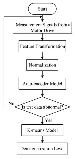
Figure 1.
Flowchart of demagnetization fault diagnosis.
This paper is organized as follows: In Section 2, the experimental setup and data processing are introduced. In Section 3, the PMSM demagnetization state is detected by using the autoencoder. In Section 4, the PMSM demagnetization level is obtained based on K-means clustering. Section 5 presents the experimental result. Finally, discussion and conclusions of the work are presented in Section 6.
2. Experimental Setup and Data Processing
To establish a machine learning model, the first step was data collection and pre-processing. This section introduces PMSM experimental setup with different demagnetization state, then the data processing methods are outlined.
2.1. Demagnetization Fault Implementation
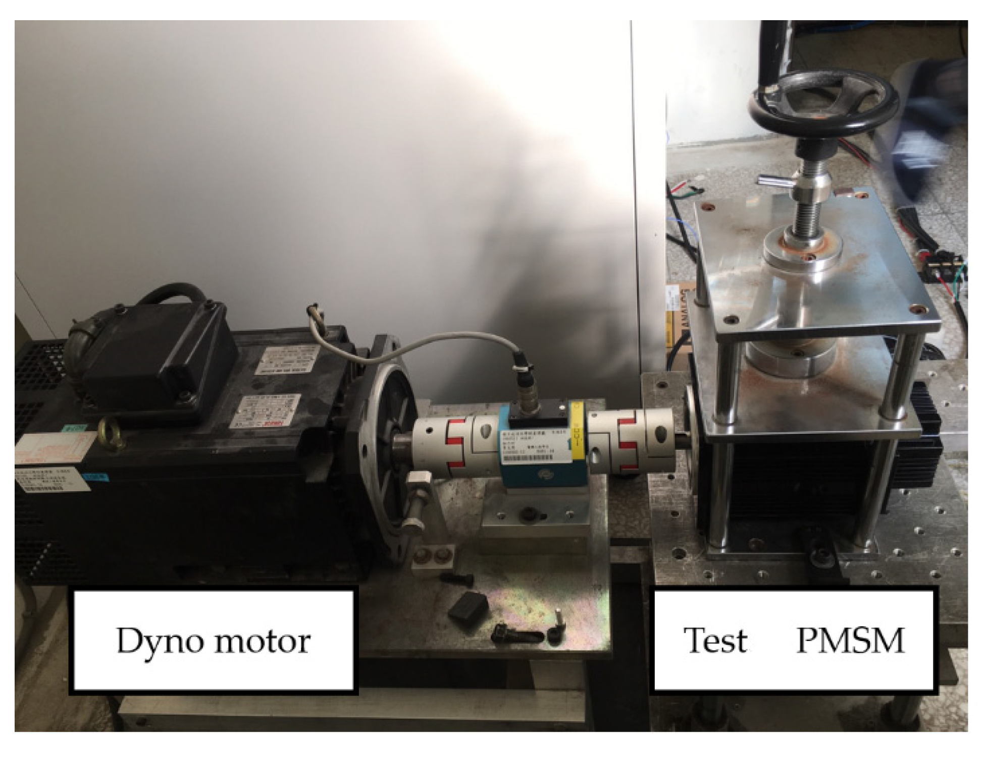
In this study, the experimental data were collected in healthy and demagnetization fault conditions. To create a demagnetization fault in a PMSM, the PMSM was fixed by a dyno motor, and a reverse excitation current was applied on d-axis to generate a reverse magnetic field [20], as shown in Figure 2.
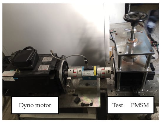
Figure 2.
Test bench to actualize demagnetization fault in a PMSM.
The specifications of the test PMSMs used in this paper are shown in Table 1, which are divided into three categories. The first is in the normal state; the second has 10% demagnetization, called the mild demagnetization fault; and the third has 25% demagnetization, called the severe demagnetization fault.

Table 1.
Specification of test PMSM.
2.2. Data Collection
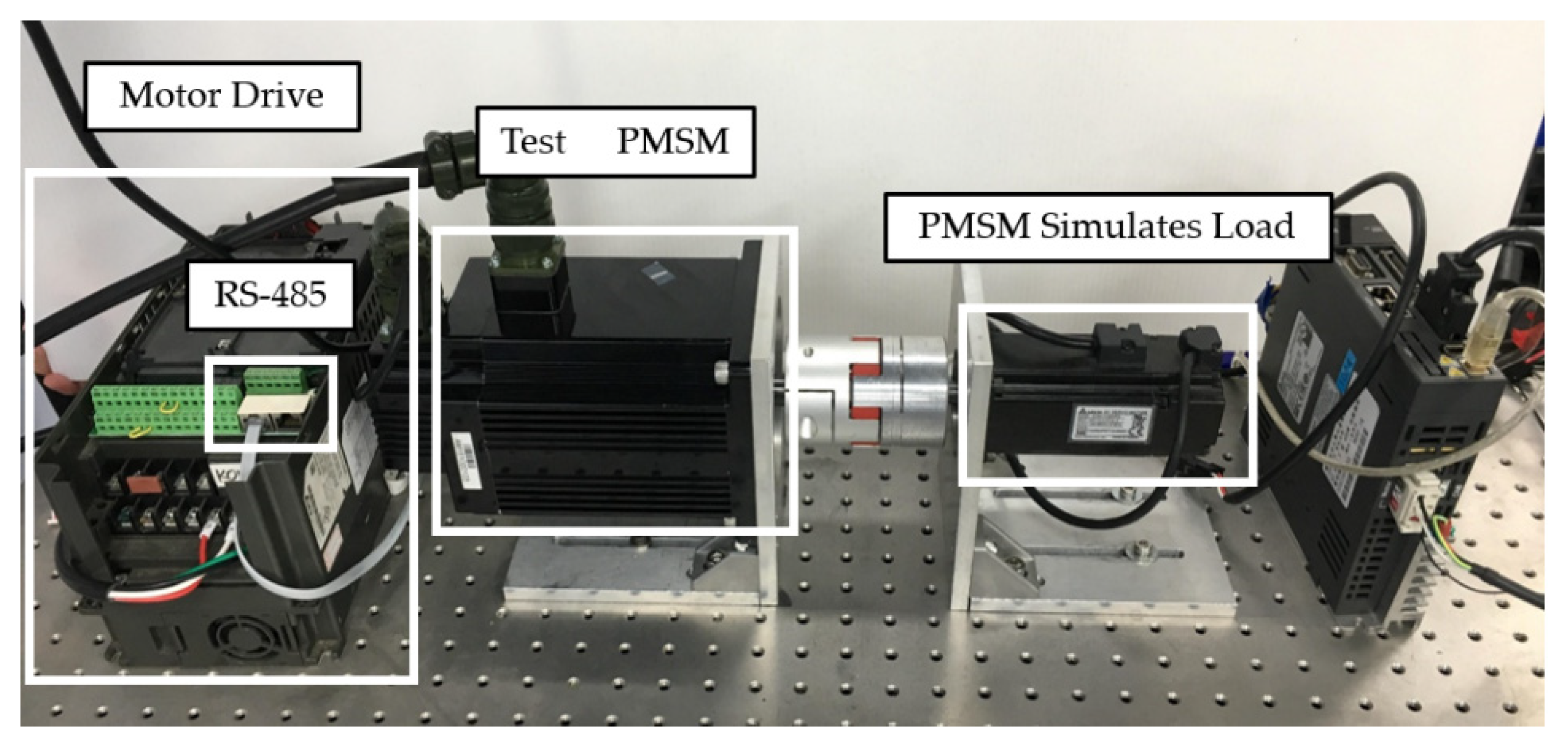
Figure 3 shows the data collection experimental setup, the test PMSM with different demagnetization degrees operated at the desired speed, and a smaller power PMSM (400 W) was controlled to give a load to the test PMSM. Both motors were operated simultaneously to collect training data.
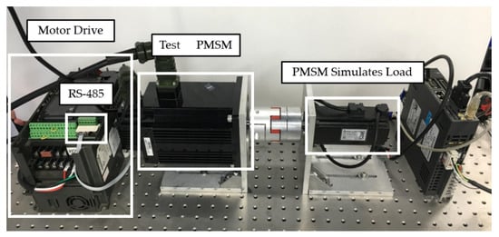
Figure 3.
Experimental setup for collecting data.
Data were acquired performed using the RS485 module for 1 s with a sampling frequency of 1000 Hz to comply with the Nyquist sampling theorem because the maximum speed of the motor was 2000 rpm and the maximum electric angular frequency was 133.33 Hz. Five physical signals (current, voltage, speed, power, and torque) were collected from the motor drive under different PMSM operation conditions. Based on the T–N curve of the test PMSM provided by the vendor, the PMSM operation is limited in the “continue duty” region during data collection, as shown in Figure 4.
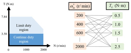
Figure 4.
PMSM operation conditions based on the T–N curve.
The data collection can be divided to two parts: training data and test data. The training data were used to train the unsupervised model (auto-encoder); thus, the data were collected from normal PMSM operation. A normal PMSM was operated at speeds between 200 and 2000 rpm and loads between 0.5 and 2.5 Nm. There was a total of 50 operation conditions, and the data collection was repeated 20 times in each operation condition; thus, 1000 datasets were obtained for training an unsupervised model. Similarly, the test data were collected from normal and demagnetized PMSM in 10 random operation conditions; thus, there were a total of 600 datasets, as shown in Table 2.

Table 2.
Classification of data collection.
2.3. Data Processing
Initially, we obtained the five physical signals: current, voltage, speed, power, and torque, from the motor drive through the RS485 module. Subsequently, we converted these five time-series signals into root mean square (RMS). It was obtained from the following expression:
where means the five physical signals, is the sampling data, and is the RMS of each 1000 sampling data.
Through the procedure of feature transformation, the original 5000 data points were compressed into five data points for reducing the data capacity. Afterward, these data were normalized by dividing the maximum current, maximum voltage, maximum speed, maximum power, and maximum torque, respectively. It was obtained from the following expression:
where means the maximum value in all , and is the normalization of the . The equation excludes the limitation of data units and improved the convergence speed and accuracy of the unsupervised learning model through normalization [21].
3. PMSM Demagnetization State Detection
This section introduces the training process of an autoencoder. Next, it describes how to fit a normal surface. Finally, the anomaly detection is presented in detail.
3.1. Autoencoder Training
We started with selecting an unsupervised learning model. The lack of need for prior labeling, effective feature extraction of data, and filtering of noise are advantages of autoencoders [22]. Therefore, we used the autoencoder as an unsupervised dimension reduction model. An autoencoder is a type of artificial neural network, and the difference between the two is that the output layer has the same number of nodes as the input layer, with the purpose of reconstructing its inputs instead of predicting the target value given inputs. Therefore, the labeling process is not required to enable learning in advance and is regarded as an unsupervised learning model. Its architecture is mainly divided into two parts: the first is a decoder and the second is an encoder. To simplify, we assume a neural network is composed of a single hidden layer. The encoder maps the input vector in the hidden representation as follows:
where is a non-linear activation function, is a weight matrix, and is a bias vector. The decoder part tries to reconstruct the input by using the following expression:
where is a weight matrix of the decoder and is the decoder bias vector. Substituting Equation (1) into Equation (2), the total autoencoder was obtained using the following expression:
The autoencoder model was trained using a training dataset composed of only normal data and minimizing the mean squared error (MSE) loss function:
where p contains all the parameters of the autoencoder, i.e., the elements of , , , and . The autoencoder previously presented is composed of only two layers: one for the encoder and one for the decoder; their number was increased to create a deep autoencoder. In general, the feature space has lower dimensionality than the input space , and the feature vector is regarded as a compressed representation of the input . Hence, we performed the dimensionality reduction through the encoder part. In this paper, the training process does not stop until the loss converges. We saved the encoder part from the trained autoencoder and the feature vector was extracted from the training dataset to the next step. The feature vector was set as three-dimensional vector to visualize the results.
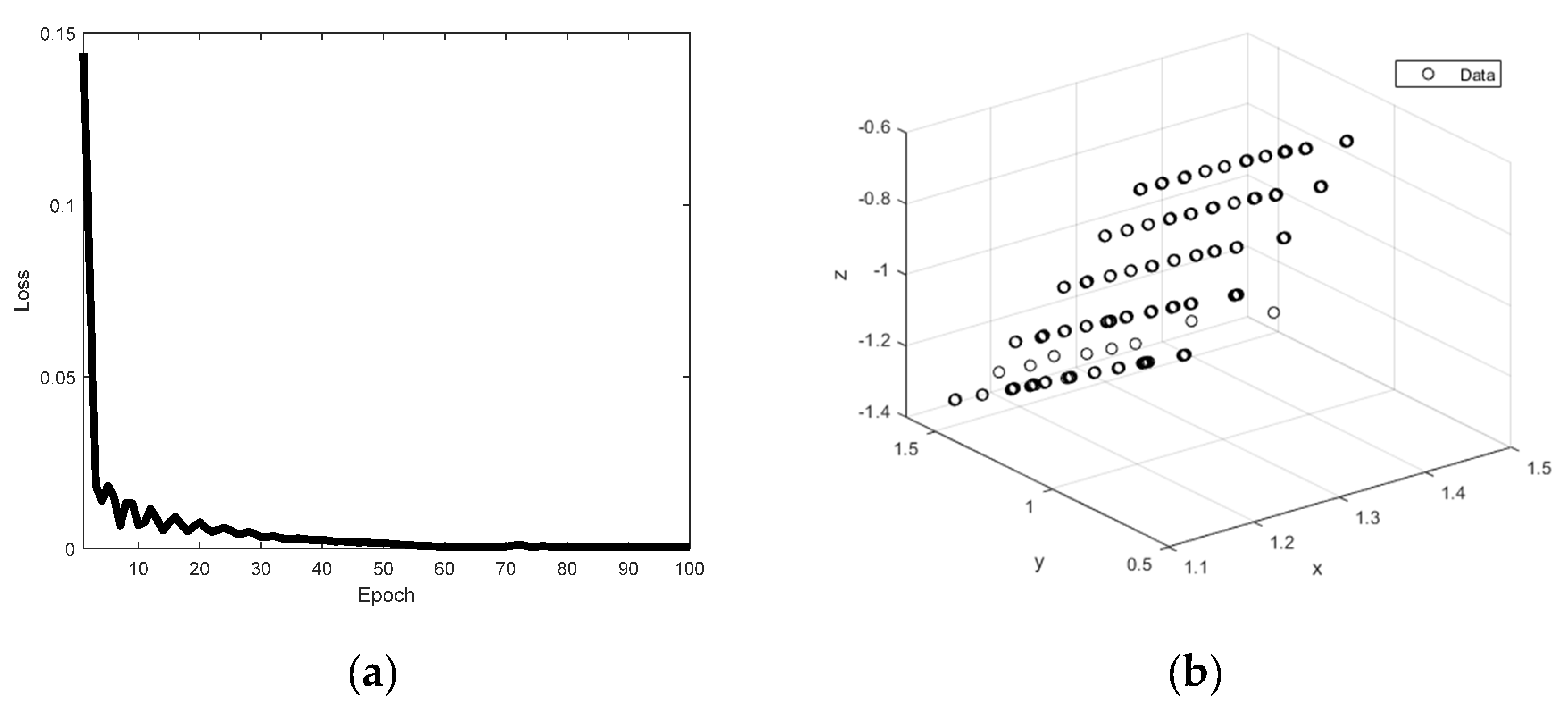
In the training process, we trained the autoencoder through the normalized training dataset composed of normal data only. The parameter settings of the proposed autoencoder are shown in Table 3. The autoencoder was trained using the Adam algorithm [23] with the learning rate of 0.001, with 100 epochs. In addition, the hyperbolic tangent function was selected as the activation function and the mean squared error was chosen as the loss function. As shown in Figure 5a, the model loss converged after training for 100 epochs. Therefore, it met the standard of completing the model training, and the three-dimensional vectors of training dataset is displayed in Figure 5b.

Table 3.
Parameter settings of the autoencoder.

Figure 5.
Results of model training: (a) model loss and (b) the three-dimensional vectors of training dataset.
3.2. Surface Fitting
Initially, we obtained the three-dimensional vector from the training dataset. Subsequently, we used the three-dimensional vector to fit a surface called the “normal surface” because the training dataset consisted of only normal data. The normal surface was obtained using the following expression:
where , , and are the three-dimensional coordinates of the space , and , , and are all the parameters of the normal surface. Fitting the normal surface was performed using the linear least squares method that minimized the sum of squared residuals [24]:
where , , and are from the three-dimensional vector . In this paper, the fitting process did not stop until the R-squared was higher than 0.9. We also saved the normal surface for the anomaly detection.
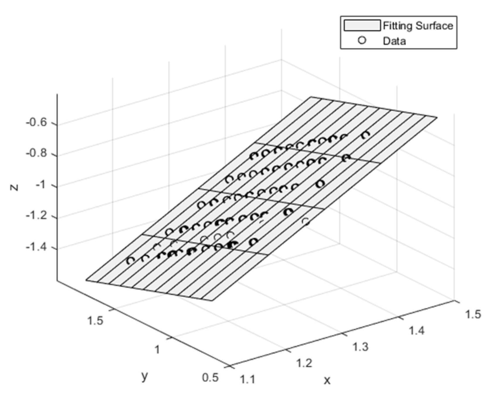
In the experiment, we fitted the normal surface with the three-dimensional vectors of training dataset and calculated some statistical metrics to evaluate the fit. Figure 6 plots the normal surface. The parameters of , , and are presented and the common statistical metrics such as the sum of squared error (SSE), root mean squared error (RMSE), and R-squared are also presented in Table 4. SSE and RMSE were close to 0, and R-squared was greater than 0.9. Hence, it met the standard of completing the surface fitting, and we saved the trained encoder and the normal surface for the purpose of anomaly detection.

Figure 6.
Normal surface.

Table 4.
Parameter settings and metrics of the normal surface.
3.3. Anomaly Detection
We started by loading the encoder that was trained during the autoencoder training stage. Next, we used the preprocessed test data as the input of the encoder. Carrying out the encoder was the last ste, to obtain the three-dimensional vector from the test data.
Next, we loaded the normal surface that was fitted in the surface fitting stage, and obtained the three-dimensional vector from the test data. After, we computed the distance from the to the normal surface from the following Equation:
where , , and are from the three-dimensional vector ; is the distance from the to the normal surface; and , , and are the parameters of the normal surface. Then, a judgement equation was constructed to determine whether the data were abnormal. The judgement equation is expressed as:
where is the threshold, is the distance from the to the normal surface. If the distance is less than or equal to the threshold , the motor state is 0, which means that the motor is under a normal state; on the contrary, if the distance is greater than the threshold , the motor state becomes one, which means that the motor is under an abnormal state. The distance between and the normal surface can determine whether demagnetization has occurred. To determine the demagnetization level, we needed to incorporate the next stage of clustering.
In the experiment, we used the preprocessed test data as the input, loaded the trained encoder, and obtained the three-dimensional vectors of test data. Figure 7 shows the three-dimensional vectors of test data.
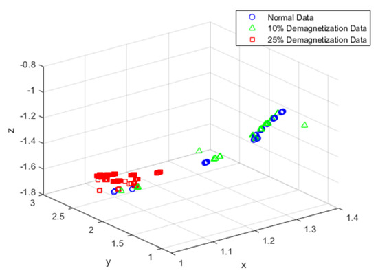
Figure 7.
Three-dimensional vectors of test data. The distribution of three test PMSMs: blue circles represent data for the normal PMSM, green triangles represent data for the PMSM with 10% demagnetization fault, and red squares represent data for PMSM with 25% demagnetization fault.
We also plotted test points on a normal surface, as shown in Figure 8a. Since the normal surface was obtained by minimizing the sum of squared residuals from training data, the maximum residual was a threshold value to determine if demagnetization had occurred. In this study, the threshold ϵ was set to 0.00102 to distinguish between normal and abnormal data. Figure 8b shows the distance from each test point to the normal surface and the threshold. In this figure, blue bars represent the distance for the normal PMSM, green bars represent the distance for the PMSM with 10% demagnetization fault, red bars represent the distance for PMSM with 25% demagnetization fault, and the black horizontal line represents the threshold. This figure also illustrates that the more the PMSM was demagnetized, the farther the distance point to the normal surface. Therefore, we used the threshold to distinguish between normal and abnormal data. The confusion matrix of anomaly detection is displayed in Table 5. In the 600 test data, 576 predictions were correct and 24 were errors. Table 6 shows the accuracy of anomaly detection; the accuracy of the normal and abnormal were 94.5%, and 96.8%, respectively. The overall accuracy of anomaly detection was 96%.
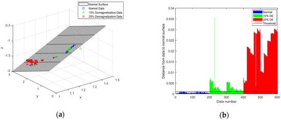
Figure 8.
Results of anomaly detection: (a) three-dimensional vectors of test data and the normal surface; (b) distance from the test data to the normal surface.

Table 5.
Confusion matrix of anomaly detection.

Table 6.
Accuracy of anomaly detection.
4. PMSM Demagnetization Level Clustering
In this study, we chose the K-means clustering as an unsupervised clustering model. This algorithm does not require prior labeling, is relatively simple to implement, scales to large datasets, and guarantees convergence [25]. The K-means algorithm is an iterative algorithm that tries to partition the dataset into K distinct non-overlapping clusters where each data point belongs to only one group. It tries to make the inter-cluster data points as similar as possible while also keeping the clusters as different as possible. It assigns data points to a cluster such that the sum of the squared distance between the data points and the cluster’s centroid is minimum. The less the variation within clusters, the more homogeneous the data points within the same cluster.
Initially, we obtained the three-dimensional vector from the test data, surmising that the motor state is abnormal from the anomaly detection. Subsequently, we used the three-dimensional vector as the input of the K-means model. Next, the model classified if the demagnetization fault in PMSM was severe. If the demagnetization fault was mild, the diagnosis system continued; however, if the demagnetization fault was severe, the diagnosis system sent a warning signal.
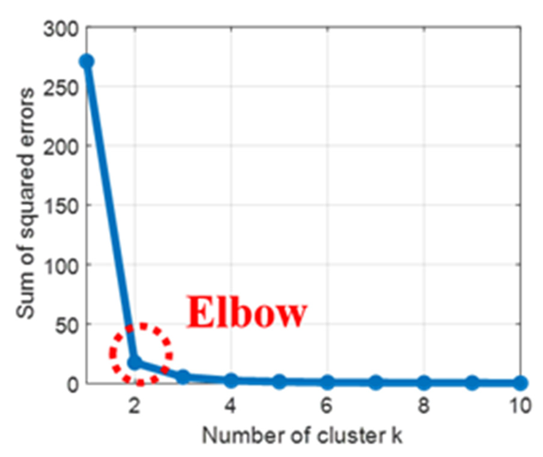
It was difficult to choose the number of clusters in the K-means clustering. Therefore, a method called elbow method was proposed by Robert in 1953. It uses the sum of squared errors (SSE) within the cluster to measure the quality of the cluster. As the number of clusters increases, the SSE in the cluster continues to decrease. This method contends that increasing the number of clusters will not enhance the effect of clustering. Therefore, there is an “elbow”, which is the optimal number of clusters.
Applying the elbow method to the abnormal test data, the experimental results are shown in Figure 9. The horizontal axis represents the number of clusters, and the vertical axis represents SSE. We observed from the figure that the most severe stage of decline is from clusters 1 to 2, and followed by a slow downward trend. Therefore, the number of clusters 2 is regarded as an elbow and also becomes the number of clusters in the K-means clustering.
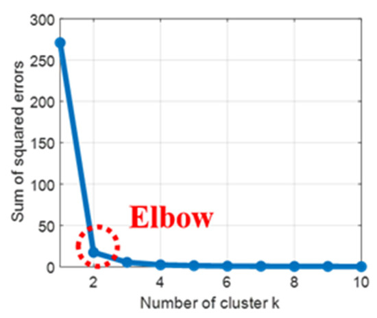
Figure 9.
Result of elbow method.
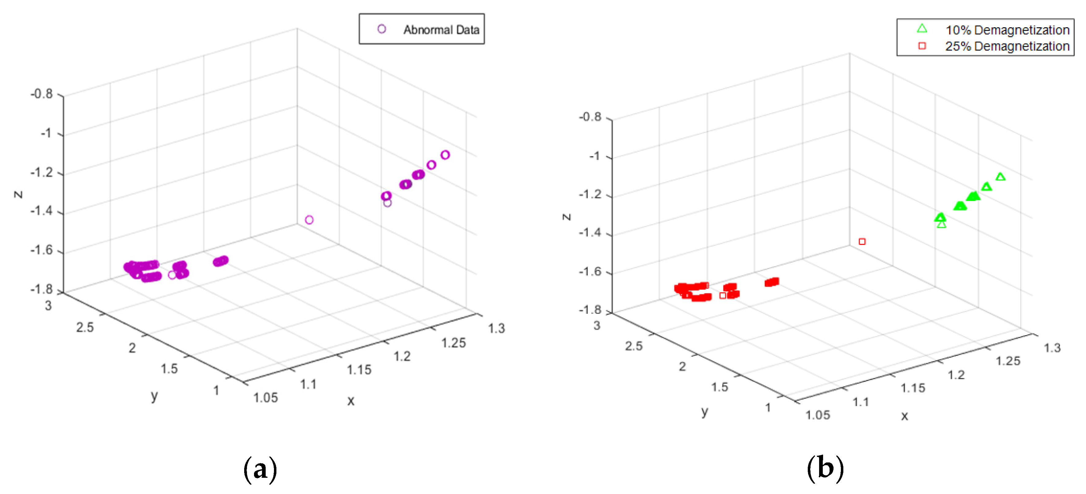
In the experiment, we obtained the three-dimensional vectors of test data considered abnormal in anomaly detection, as shown in Figure 10a. Then, K-means clustering was used for clustering. Figure 10b displayed the result of the K-means clustering, and we found that the abnormal data was divided into two clusters: one cluster was mainly composed of the PMSM with 10% demagnetization fault; the second cluster was mainly composed of the PMSM with 25% demagnetization fault. The confusion matrix of clustering is displayed in Table 7. Of the 398 test data considered abnormal, 386 predictions were correct and 12 were errors. Table 8 shows the accuracy of clustering, the accuracies of the PMSM with 10% demagnetization fault and the PMSM with 25% demagnetization fault were 99.5%, and 100%, respectively. The overall accuracy of clustering was 97%.
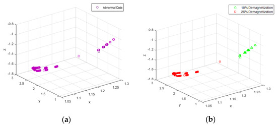
Figure 10.
Clustering: (a) data considered abnormal in anomaly detection and (b) results of clustering.

Table 7.
Confusion matrix of clustering.

Table 8.
Accuracy of clustering.
5. Experimental Results
Combining the anomaly detection and clustering, the confusion matrix of the total test data is summarized in Table 9. Of the 600 test data, 575 predictions were correct and 25 were errors. Table 10 shows the accuracy of test dataset, the normal PMSM, the PMSM with 10% demagnetization fault, and the PMSM with 25% demagnetization fault: 94.5%, 93%, and 100%, respectively. The overall accuracy of our proposed method was 96%. The experimental results showed that the proposed unsupervised demagnetization fault diagnosis system in PMSM can accurately diagnose demagnetization faults in a real environment.

Table 9.
Confusion matrix of test dataset.

Table 10.
Accuracy of test dataset.
6. Conclusions
In this paper, an unsupervised demagnetization fault diagnosis method in PMSM was proposed. The unsupervised learning method was adopted to help simplify label engineering in training process, unlike recent research that often uses supervised learning methods. To reduce costs, five different physical signals were captured directly from the motor driver as training data and test data as opposed to the method used in the literature, [4] which only adopts a stator current signal. Multiple physical signals were used simultaneously that reduced the influence of data noise compared to using single physical signal.
In this study, the PMSM demagnetization fault diagnosis was performed in three states: normal, 10% demagnetization fault, and 25% demagnetization fault. More than 1000 training data points were used for training the algorithm and 600 for testing. The experimental results showed that the accuracy of anomaly detection was 96%, the accuracy of clustering was 97%, and the accuracy of total diagnosis system was 96%. The experimental results confirmed that the proposed method is feasible for PMSM demagnetization fault diagnosis.
Author Contributions
Conceptualization, L.-K.C. and M.-C.T.; methodology, L.-K.C. and S.-H.W.; validation, S.-H.W.; data curation, S.-H.W.; writing—original draft preparation, L.-K.C. and S.-H.W.; writing—review and editing, L.-K.C.; supervision, M.-C.T.; project administration, L.-K.C. and M.-C.T. All authors have read and agreed to the published version of the manuscript.
Funding
This work was funded by [Ministry of Science and Technology, R.O.C.] grant number [MOST 108-2622-8-006-014].
Acknowledgments
This work was supported by the Ministry of Science and Technology, R.O.C. (grant number MOST 108-2622-8-006-014).
Conflicts of Interest
The authors declare no conflict of interest.
References
- Ishikawa, T.; Igarashi, N. Failure Diagnosis of Demagnetization in Interior Permanent Magnet Synchronous Motors Using Vibration Characteristics. Appl. Sci. 2019, 9, 3111. [Google Scholar] [CrossRef]
- Zhu, M.; Hu, W.S.; Kar, N.C. Acoustic Noise-Based Uniform Permanent-Magnet Demagnetization Detection in SPMSM for High-Performance PMSM Drive. IEEE Trans. Transp. Electrif. 2018, 4, 1397–1405. [Google Scholar] [CrossRef]
- Maraaba, L.; Al-Hamouz, Z.; Abido, M. An efficient stator inter-turn fault diagnosis tool for induction motors. Energies 2018, 11, 653. [Google Scholar] [CrossRef]
- Liang, H.; Chen, Y.; Liang, S.; Wang, C. Fault detection of stator inter-turn short-circuit in PMSM on stator current and vibration signal. Appl. Sci. 2018, 8, 1677. [Google Scholar] [CrossRef]
- Liang, S.; Chen, Y.; Liang, H.; Li, X. Sparse Representation and SVM Diagnosis Method for Inter-Turn Short-Circuit Fault in PMSM. Appl. Sci. 2019, 9, 224. [Google Scholar] [CrossRef]
- Zhen, D.; Wang, Z.; Li, H.; Zhang, H.; Yang, J.; Gu, F. An Improved Cyclic Modulation Spectral Analysis Based on the CWT and Its Application on Broken Rotor Bar Fault Diagnosis for Induction Motors. Appl. Sci. 2019, 9, 3902. [Google Scholar] [CrossRef]
- Ruiz, J.R.; Rosero, J.A.; Espinosa, A.G.; Romeral, L. Detection of Demagnetization Faults in Permanent-Magnet Synchronous Motors Under Nonstationary Conditions. IEEE Trans. Magn. 2009, 45, 2961–2969. [Google Scholar] [CrossRef]
- Momeni, H.; Sadoogi, N.; Farrokhifar, M.; Gharibeh, H.F. Fault diagnosis in photovoltaic arrays using GBSSL method and proposing a fault correction system. IEEE Trans. Ind. Inf. 2019, 16, 5300–5308. [Google Scholar] [CrossRef]
- Xu, X.; Zhao, Z.; Xu, X.; Yang, J.; Chang, L.; Yan, X.; Wang, G. Machine learning-based wear fault diagnosis for marine diesel engine by fusing multiple data-driven models. Knowl. Based Syst. 2020, 190, 105324. [Google Scholar] [CrossRef]
- Jegadeeshwaran, R.; Sugumaran, V. Fault diagnosis of automobile hydraulic brake system using statistical features and support vector machines. Mech. Syst. Signal Process. 2015, 52, 436–446. [Google Scholar] [CrossRef]
- Ataei, M.; Kiyoumarsi, A.; Ghorbani, B. Control of chaos in permanent magnet synchronous motor by using optimal Lyapunov exponents placement. Phys. Lett. A 2010, 374, 4226–4230. [Google Scholar] [CrossRef]
- Kao, I.H.; Wang, W.J.; Lai, Y.H.; Perng, J.W. Analysis of permanent magnet synchronous motor fault diagnosis based on learning. IEEE Trans. Instrum. Meas. 2019, 68, 310–324. [Google Scholar] [CrossRef]
- Skowron, M.; Wolkiewicz, M.; Orlowska-Kowalska, T.; Kowalski, C.T. Effectiveness of Selected Neural Network Structures Based on Axial Flux Analysis in Stator and Rotor Winding Incipient Fault Detection of Inverter-fed Induction Motors. Energies 2019, 12, 2392. [Google Scholar] [CrossRef]
- Dybkowski, M.; Klimkowski, K. Artificial Neural Network Application for Current Sensors Fault Detection in the Vector Controlled Induction Motor Drive. Sensors 2019, 19, 571. [Google Scholar] [CrossRef] [PubMed]
- Burriel-Valencia, J.; Puche-Panadero, R.; Martinez-Roman, J.; Sapena-Bano, A.; Pineda-Sanchez, M.; Perez-Cruz, J.; Riera-Guasp, M. Automatic fault diagnostic system for induction motors under transient regime optimized with expert systems. Electronics 2019, 8, 6. [Google Scholar] [CrossRef]
- Zolfaghari, S.; Noor, S.B.M.; Rezazadeh Mehrjou, M.; Marhaban, M.H.; Mariun, N. Broken rotor bar fault detection and classification using wavelet packet signature analysis based on fourier transform and multi-layer perceptron neural network. Appl. Sci. 2018, 8, 25. [Google Scholar] [CrossRef]
- Hsueh, Y.M.; Ittangihal, V.R.; Wu, W.B.; Chang, H.C.; Kuo, C.C. Fault diagnosis system for induction motors by CNN using empirical wavelet transform. Symmetry 2019, 11, 1212. [Google Scholar] [CrossRef]
- Hsueh, Y.; Ittangihala, V.R.; Wu, W.B.; Chang, H.C.; Kuo, C.C. Condition Monitor System for Rotation Machine by CNN with Recurrence Plot. Energies 2019, 12, 3221. [Google Scholar] [CrossRef]
- Lee, J.H.; Pack, J.H.; Lee, I.S. Fault Diagnosis of Induction Motor Using Convolutional Neural Network. Appl. Sci. 2019, 9, 2950. [Google Scholar] [CrossRef]
- Chattopadhyay, S.; Mitra, M.; Sengupta, S. Clarke and park transform. In Electric Power Quality; Springer: Berlin/Heidelberg, Germany, 2011; pp. 89–96. [Google Scholar]
- Khan, U.; Safari, P.; Hernando, J. Restricted Boltzmann Machine Vectors for Speaker Clustering and Tracking Tasks in TV Broadcast Shows. Appl. Sci. 2019, 9, 2761. [Google Scholar] [CrossRef]
- Wold, S.; Esbensen, K.; Geladi, P. Principal component analysis. Chemom. Intell. Lab. Syst. 1987, 2, 37–52. [Google Scholar] [CrossRef]
- Ba, J.; Adam-Kingma, D.P. A method for stochastic optimization. In Proceedings of the International Conference on Machine Learning (ICML), San Diego, CA, USA, 17 June 2015. [Google Scholar]
- Nwankwo, L.I. A least square plane surface polynomial fit of two dimensional potential field geophysical data using Matlab. Niger. J. Pure Appl. Sci. 2006, 21, 2006–2013. [Google Scholar]
- Jain, A.K.; Murty, M.N.; Flynn, P.J. Data clustering: A review. ACM Comput. Surv. CSUR 1999, 31, 264–323. [Google Scholar] [CrossRef]
© 2020 by the authors. Licensee MDPI, Basel, Switzerland. This article is an open access article distributed under the terms and conditions of the Creative Commons Attribution (CC BY) license (http://creativecommons.org/licenses/by/4.0/).


