A Modified Reynolds-Averaged Navier–Stokes-Based Wind Turbine Wake Model Considering Correction Modules


Abstract
1. Introduction
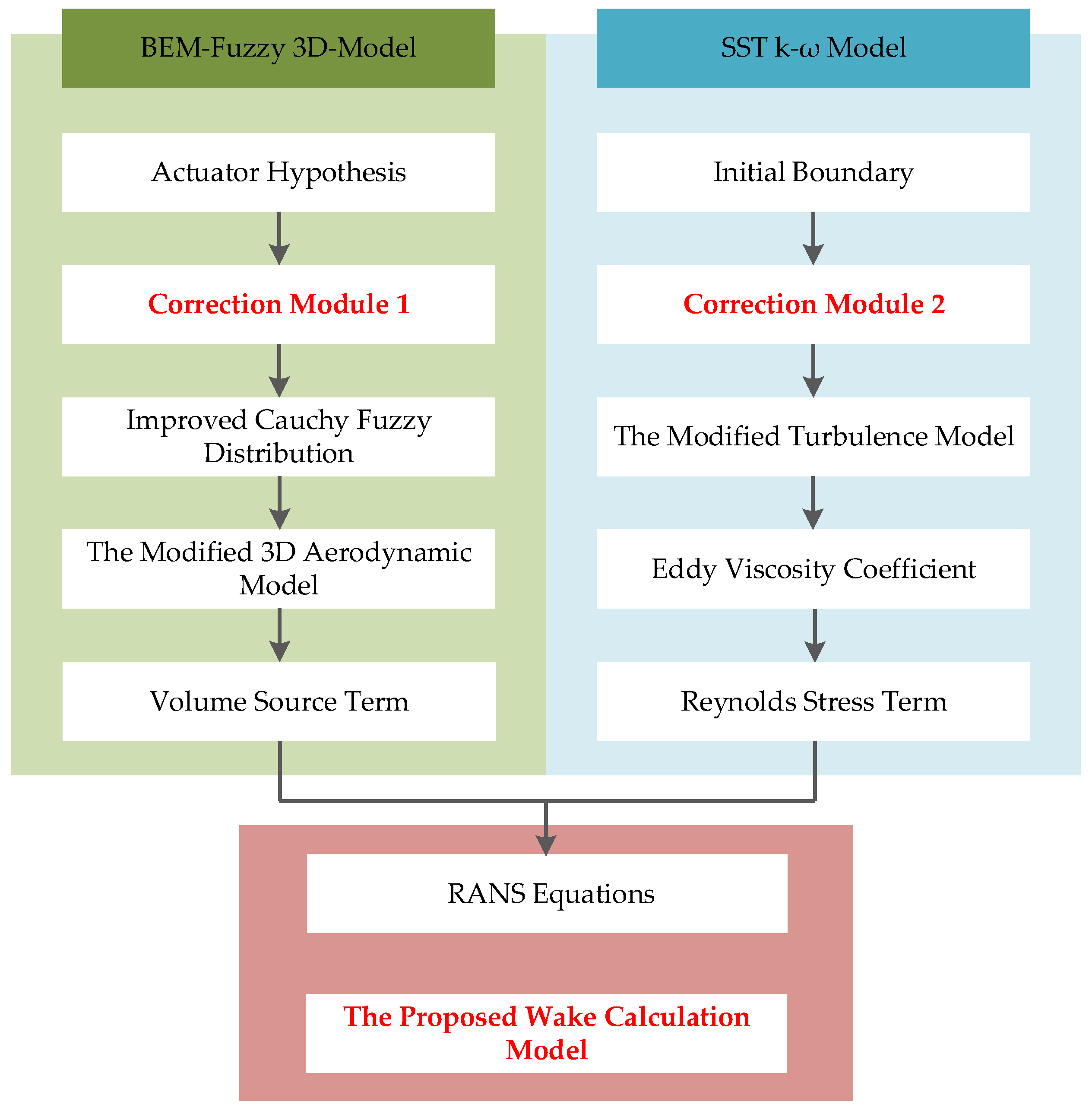
- This paper proposes a modified Reynolds-averaged Navier–Stokes (MRANS)-based wind turbine wake model to simulate the wake effects. Based on the correction module, the proposed blade element momentum (BEM) -fuzzy aerodynamic model can amend the inconsistent condition between the wake simulation and the experiment test. For the turbulence model, the turbulence attenuation is effectively avoided by adding the hold source term. The accuracy of the turbulence intensity distribution is improved by correcting the closure constant and the dissipation term.
- Simulation results of the velocity field and turbulent field with the proposed approach are consistent with the data of real wind turbines, which verifies the effectiveness of the proposed approach. Furthermore, the computation efficiency is significantly improved by the developed mesh partition method.
2. Overall Wind Turbine Wake Model
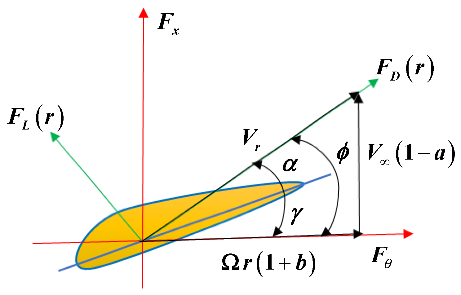
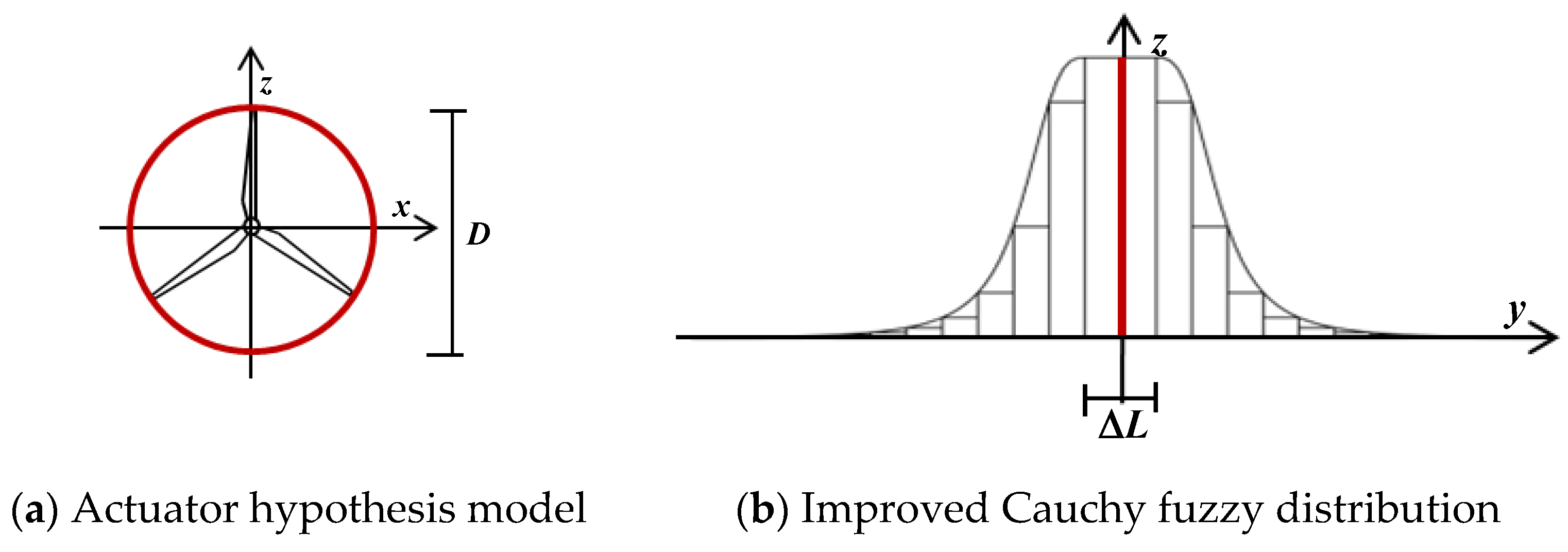
3. BEM-Fuzzy 3D Aerodynamic Model
3.1. Tip Loss Correction
3.2. Hub Loss Correction
3.3. Attack Angle Correction
4. SST k-ω Turbulence Model
4.1. Hold Source Term
4.2. Closure Constant Correction
4.3. Correction Factor Addition
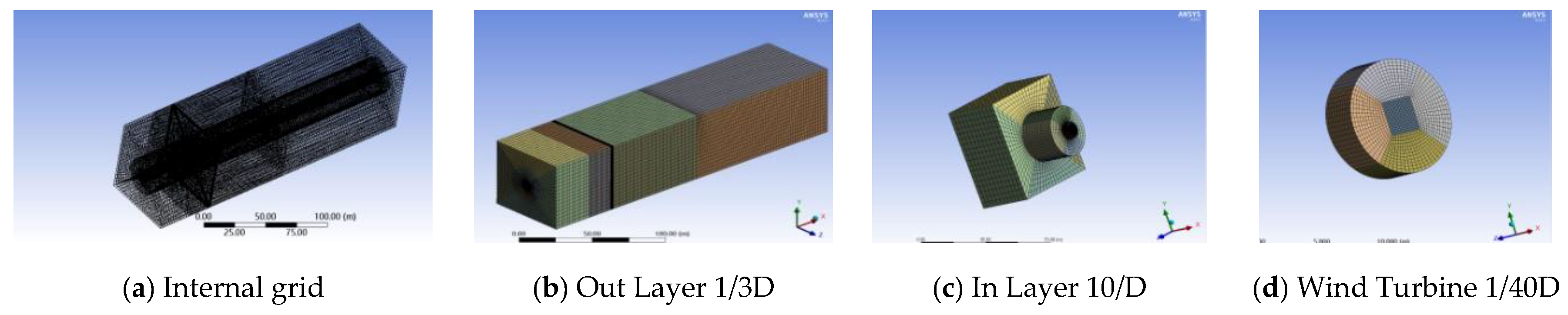
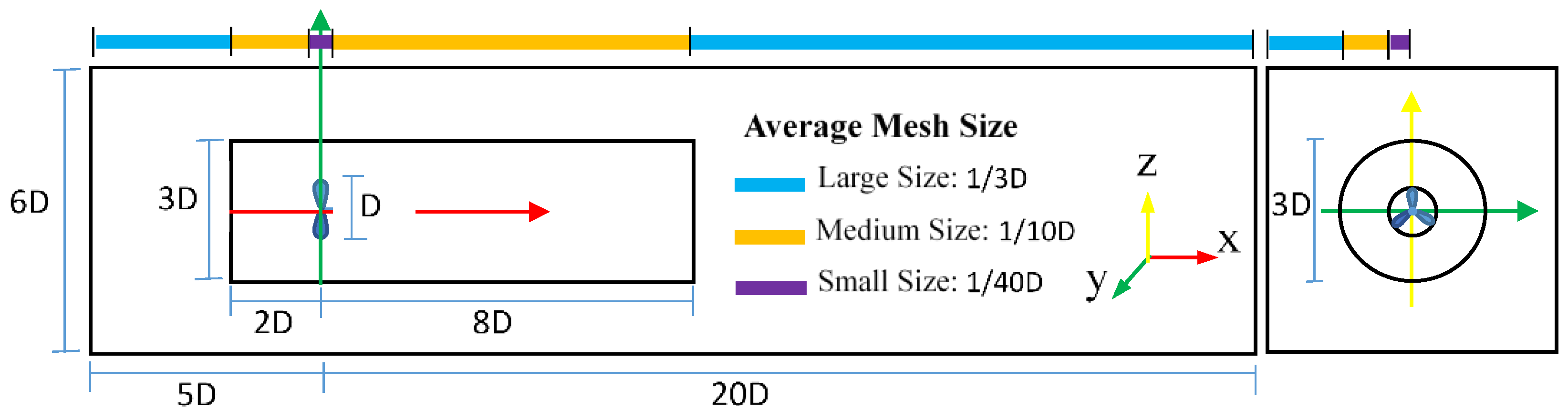
5. Mesh Partition Method
6. Simulation Results
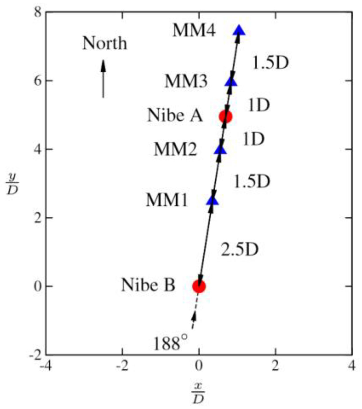
6.1. Simulation Setup
6.2. Velocity Field under the Uniform Inflow Condition
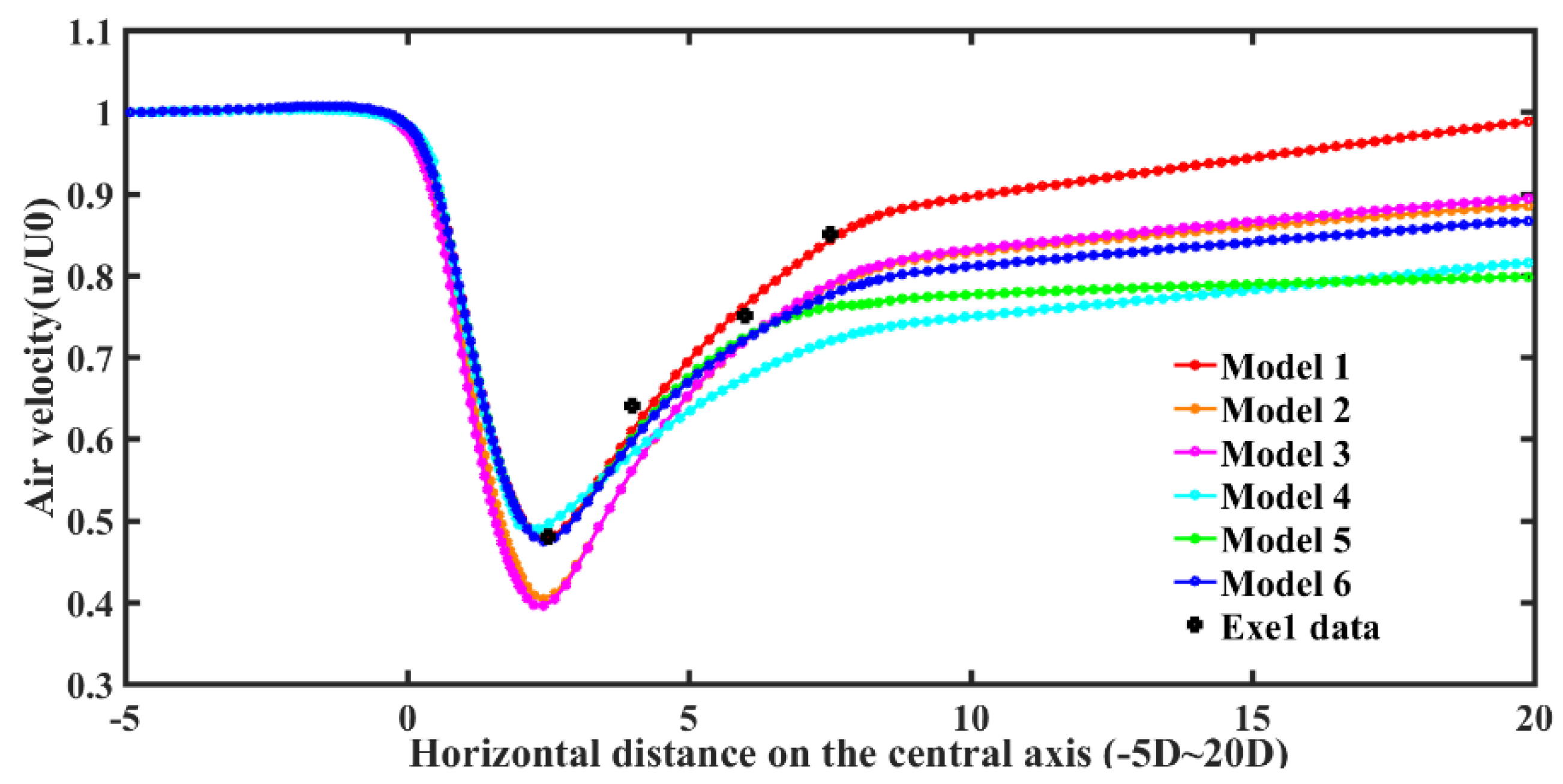
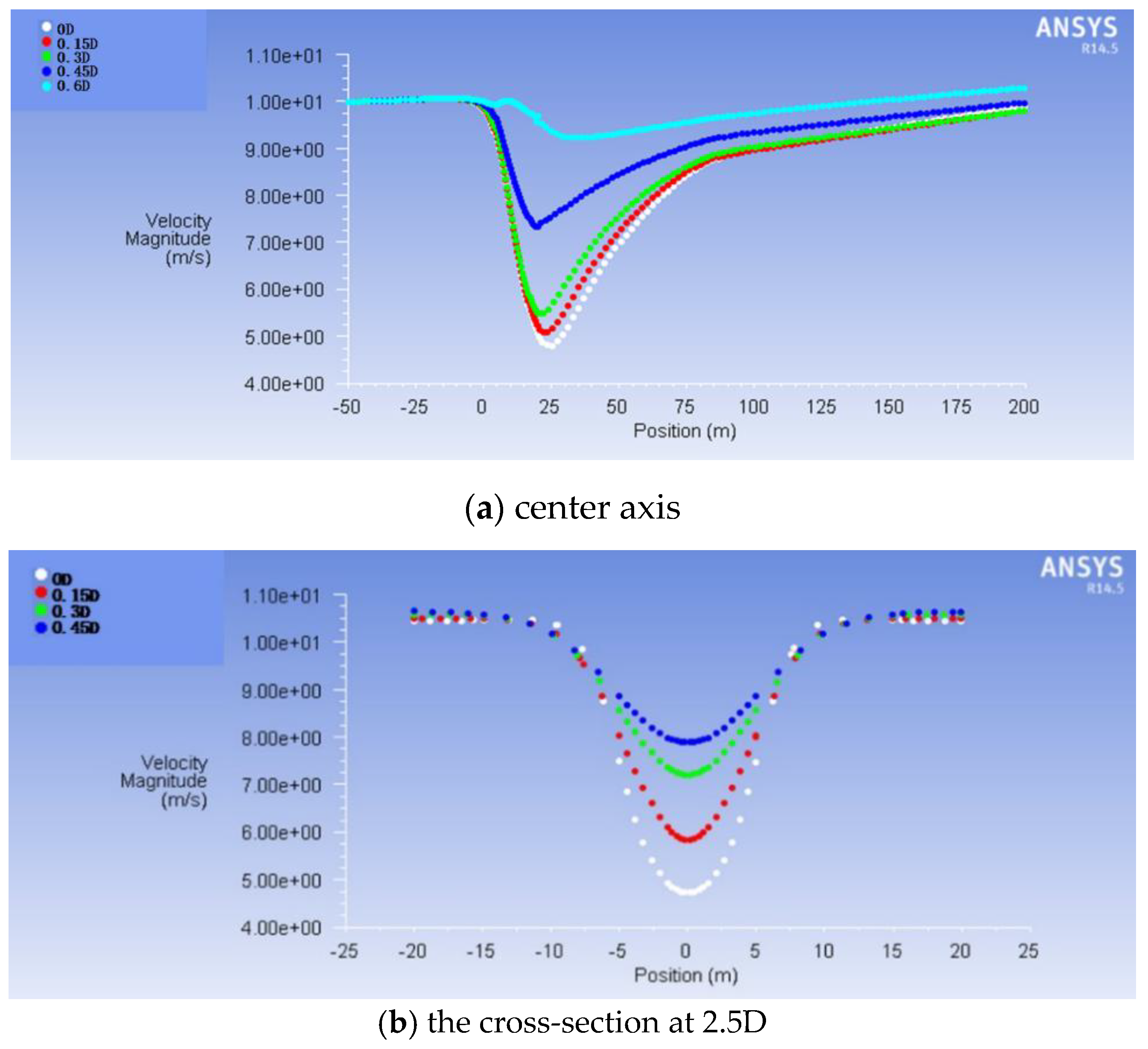
6.2.1. Comparison and Analysis of Velocity Field Results at the Center Axis
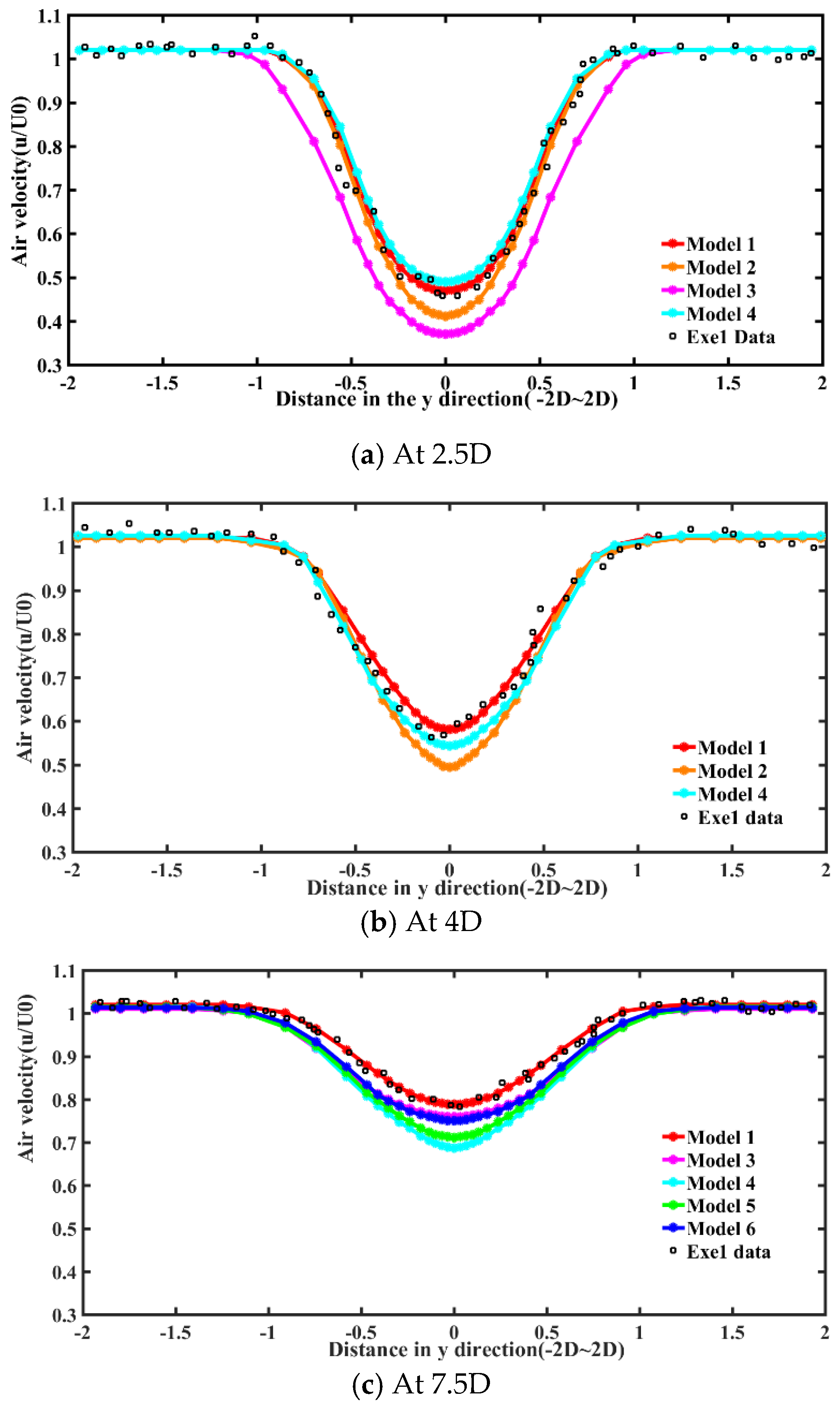
6.2.2. Correction Velocity Results at the Different Cross-Sections of Axial Direction
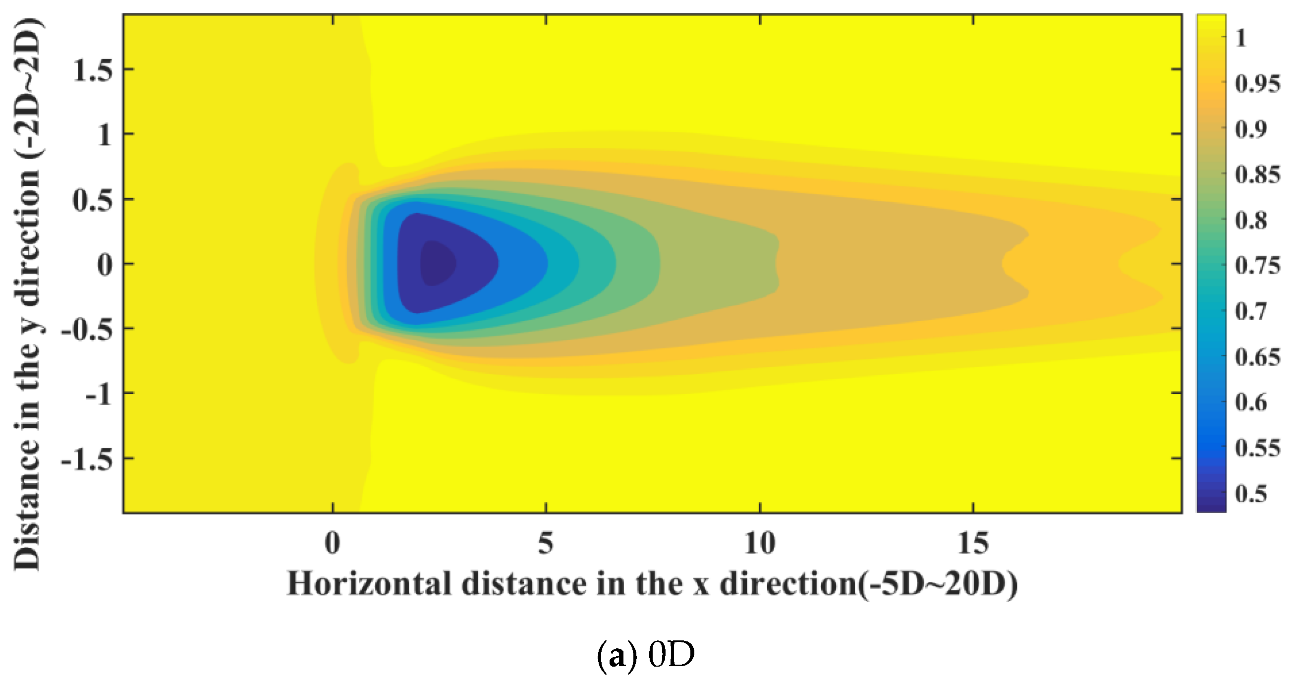
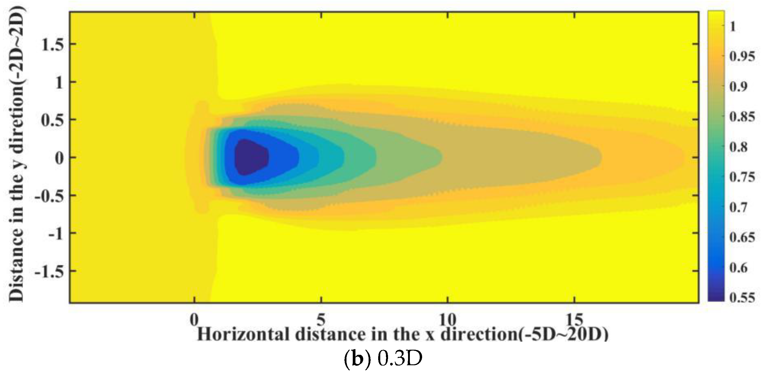
6.2.3. Velocity at Different Altitudes
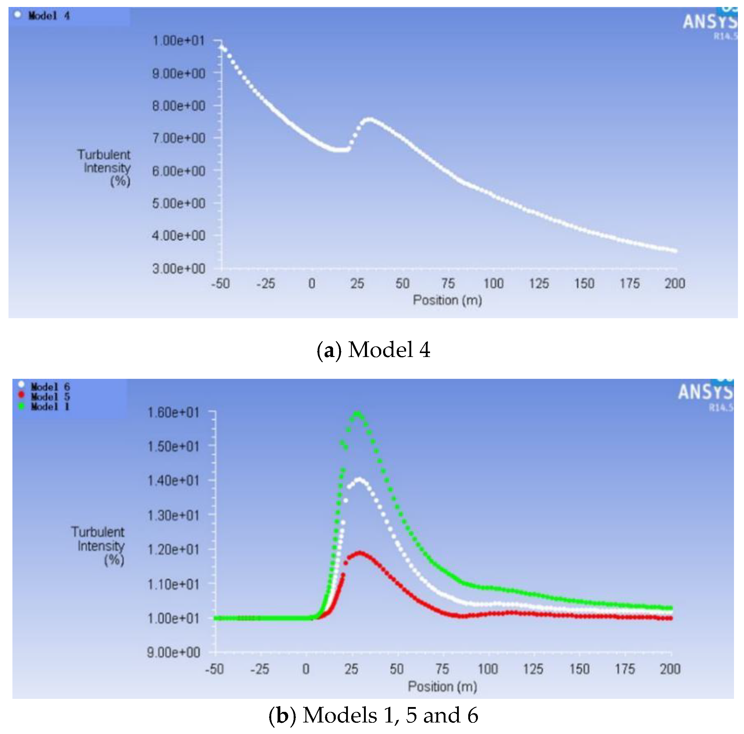
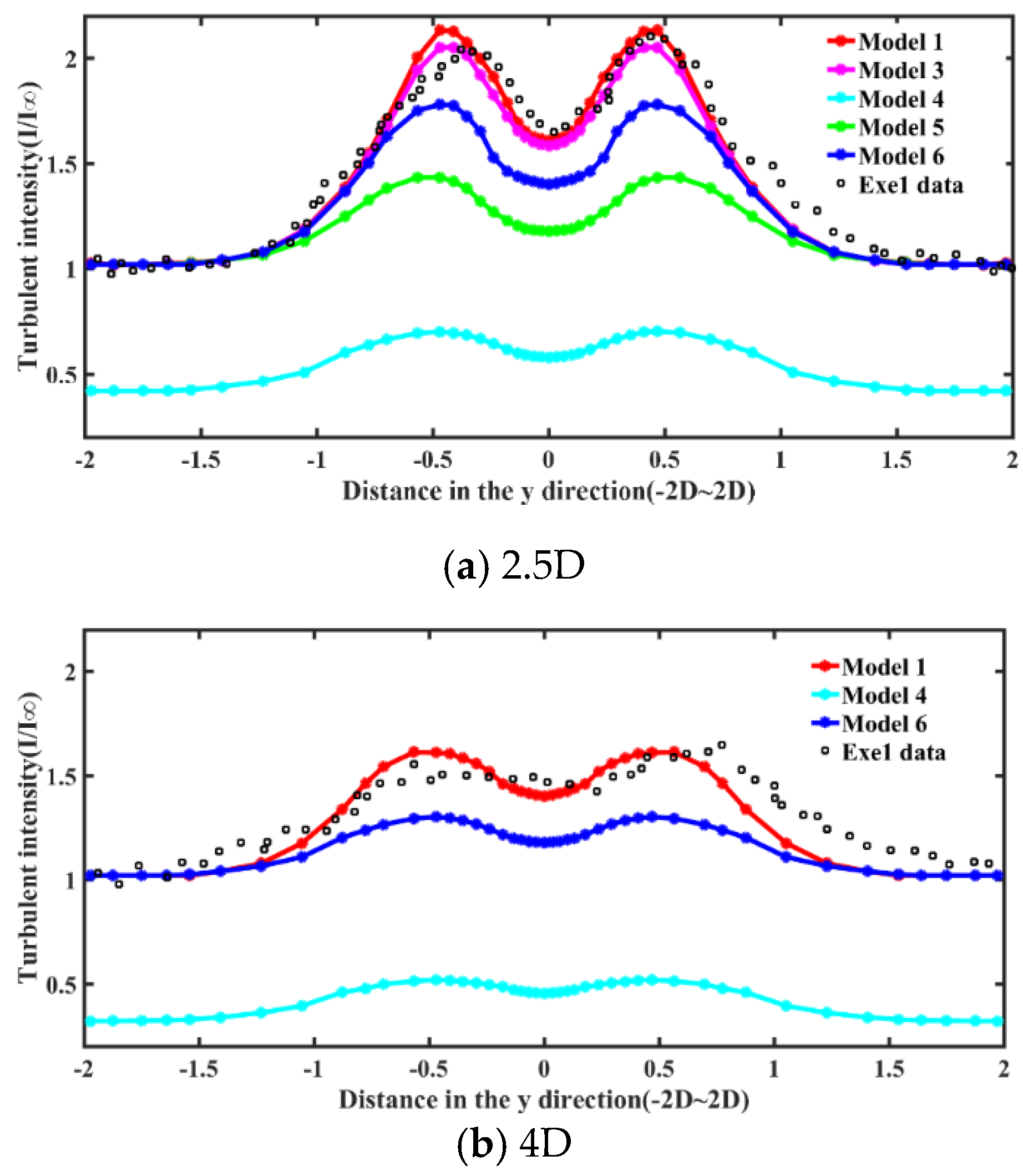
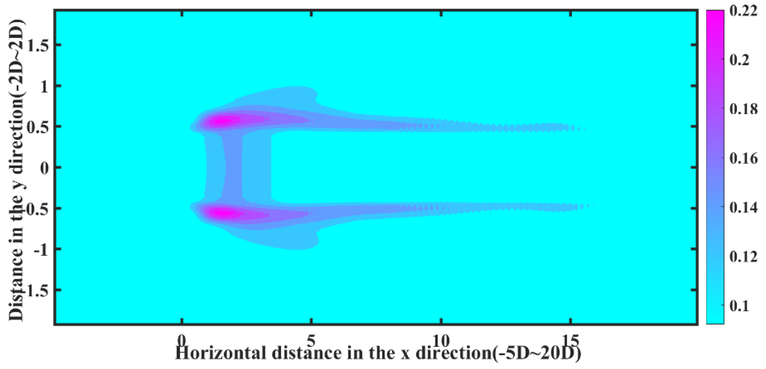
6.3. Turbulence Field Result under the Uniform Inflow Condition
6.4. Computation Evaluation
7. Conclusions
Author Contributions
Funding
Conflicts of Interest
References
- Barthelmie, R.J.; Frandsen, S.T.; Nielsen, M.N.; Pryor, S.C.; Rethore, P.E.; Jørgensen, H.E. Modelling and measurements of power losses and turbulence intensity in wind turbine wakes at Middelgrunden offshore wind farm. Wind Energy 2007, 10, 517–528. [Google Scholar] [CrossRef]
- Shao, Z.; Wu, Y.; Li, L.; Han, S.; Liu, Y. Multiple wind turbine wakes modeling considering the faster wake recovery in overlapped wakes. Energies 2019, 12, 680. [Google Scholar] [CrossRef]
- Tao, S.; Kuenzel, S.; Xu, Q.; Chen, Z. Optimal micro-siting of wind turbines in an offshore wind farm using Frandsen-Gaussian wake model. IEEE Trans. Power Syst. 2019, 34, 4944–4954. [Google Scholar] [CrossRef]
- Wang, H.; Yang, J.; Chen, Z.; Ge, W.; Hu, S.; Ma, Y.; Li, Y.; Zhang, G.; Yang, L. Gain scheduled torque compensation of pmsg-based wind turbine for frequency regulation in an isolated grid. Energies 2018, 11, 1623. [Google Scholar] [CrossRef]
- Hand, B.; Cashman, A.; Kelly, G. A low-order model for offshore floating vertical axis wind turbine aerodynamics. IEEE Trans. Ind. Appl. 2017, 53, 512–520. [Google Scholar] [CrossRef]
- Wang, X.; Gao, W.; Scholbrock, A.; Muljadi, E.; Gevorgian, V.; Wang, J.; Yan, W.; Zhang, H. Evaluation of different inertial control methods for variable-speed wind turbines simulated by fatigue, aerodynamic, structures and turbulence (FAST). IET Renew. Power Gener. 2017, 11, 1534–1544. [Google Scholar] [CrossRef]
- Behrouzifar, A.; Darbandi, M. An improved actuator disc model for the numerical prediction of the far-wake region of a horizontal axis wind turbine and its performance. Energy Convers. Manag. 2019, 18, 482–495. [Google Scholar] [CrossRef]
- Castellani, F.; Astolfi, D.; Mana, M.; Piccioni, E. Investigation of terrain and wake effects on the performance of wind farms in complex terrain using numerical and experimental data. Wind Energy 2017, 20, 1277–1289. [Google Scholar]
- Sedaghatizadeh, N.; Arjomandi, M.; Kelso, R.; Cazzolato, B.; Ghayesh, M.H. The effect of the boundary layer on the wake of a horizontal axis wind turbine. Energy 2019, 18, 1202–1221. [Google Scholar] [CrossRef]
- Reda, S.; Teng, W. A semi-empirical model for mean wind velocity profile of landfalling hurricane boundary layers. J. Wind Eng. Ind. Aerodyn. 2018, 180, 249–261. [Google Scholar]
- Zhang, Y.; Ye, Z.; Li, C. Wind turbine aerodynamic performance simulation based on improved lifting surface free wake method. Acta Energ. Sol. Sin. 2017, 38, 1316–1323. [Google Scholar]
- Zhang, Y.; Fernandez-Rodriguez, E.; Zheng, J.; Zheng, Y.; Zhang, J.; Gu, H.; Zang, W.; Lin, X. A review on numerical development of tidal stream turbine performance and wake prediction. IEEE Access 2020, 8, 79325–79337. [Google Scholar] [CrossRef]
- Laan, M.P.; Sørensen, N.N.; Réthoré, P. An improved k-ε model applied to a wind turbine wake in atmospheric turbulence. Wind Energy 2015, 18, 889–907. [Google Scholar] [CrossRef]
- Almohammadi, K.M.; Ingham, D.B.; Ma, L.; Pourkashanian, M. 2-D-CFD analysis of the effect of trailing edge shape on the performance of a straight-blade vertical axis wind turbine. IEEE Trans. Sustain. Energy 2015, 6, 228–235. [Google Scholar] [CrossRef]
- Yin, X.; Zhao, X. Deep neural learning based distributed predictive control for offshore wind farm using high fidelity LES data. IEEE Trans. Ind. Electron. 2020. [Google Scholar] [CrossRef]
- Seim, F.; Gravdahl, A.R.; Adaramola, M.S. Validation of kinematic wind turbine wake models in complex terrain using actual windfarm production data. Energy 2017, 123, 742–753. [Google Scholar] [CrossRef]
- Kleusberg, E.; Mikkelsen, R.F.; Schlatter, P.; Ivanell, S. High-order numerical simulations of wind turbine wakes. J. Phys. Conf. 2017, 854, 012025. [Google Scholar] [CrossRef]
- Barrett, R.; Ning, A. Comparison of airfoil precomputational analysis methods for optimization of wind turbine blades. IEEE Trans. Sustain. Energy 2016, 7, 1081–1088. [Google Scholar] [CrossRef]
- Arteaga-López, E.; Ángeles-Camacho, C.; Bañuelos-Ruedas, F. Advanced methodology for feasibility studies on building-mounted wind turbines installation in urban environment: Applying CFD analysis. Energy 2019, 16, 181–188. [Google Scholar] [CrossRef]
- Liang, H.; Zuo, L.; Li, J.; Li, B.C.; He, Y.; Huang, Q. A wind turbine control method based on Jensen model. In Proceedings of the 2016 International Conference on Smart Grid and Clean Energy Technologies (ICSGCE), Chengdu, China, 19–22 October 2016; IEEE: Piscataway, NJ, USA, 2016. [Google Scholar]
- Sørensen, O.; Jacob, B. Linearised CFD Models for Wakes; Risø National Laboratory: Roskilde, Denmark, 2011. [Google Scholar]
- Johansen, J.; Sørensen, N.N.; Michelsen, J.A. Detached-eddy simulation of flow around the NREL Phase VI blade. Wind Energy 2002, 5, 185–197. [Google Scholar] [CrossRef]
- Sarlak, H.; Meneveau, C.; Sorensen, J.N. Role of subgrid-scale modeling in large eddy simulation of wind turbine wake interactions. Renew. Energy 2015, 77, 386–399. [Google Scholar] [CrossRef]
- Mo, J.O.; Choudhry, A.; Arjomandi, M.; Lee, Y. Adelaide Research and Scholarship: Large Eddy Simulation of the Wind Turbine Wake Characteristics in the Numerical Wind Tunnel Model; Elsevier Science Bv: Amsterdam, The Netherlands, 2013. [Google Scholar]
- Zhang, B.; Soltani, M.; Hu, W.; Hou, P.; Huang, Q.; Chen, Z. Optimized power dispatch in wind farms for power maximizing considering fatigue loads. IEEE Trans. Sustain. Energy 2018, 9, 862–871. [Google Scholar] [CrossRef]
- Farhan, A.; Hassanpour, A.; Burns, A.; Motlagh, Y.G. Numerical study of effect of winglet planform and airfoil on a horizontal axis wind turbine performance. Renew. Energy 2019, 13, 1255–1273. [Google Scholar] [CrossRef]
- Lee, H.; Lee, D.J. Numerical investigation of the aerodynamics and wake structures of horizontal axis wind turbines by using nonlinear vortex lattice method. Renew. Energy 2019, 13, 1121–1133. [Google Scholar] [CrossRef]
- Tang, D.; Xu, M.; Mao, J.; Zhu, H. Unsteady performances of a parked large-scale wind turbine in the typhoon activity zones. Renew. Energy 2020, 14, 617–630. [Google Scholar] [CrossRef]
- Roggenburg, M.; Esquivel-Puentes, H.A.; Vacca, A.; Evans, H.B.; Garcia-Bravo, J.M.; Warsinger, D.M.; Ivantysynova, M.; Castillo, L. Techno-economic analysis of a hydraulic transmission for floating offshore wind turbines. Renew. Energy 2020, 15, 1194–1204. [Google Scholar] [CrossRef]
- El-Askary, W.A.; Sakr, I.M.; Abdelsalam, A.M.; Abuhegazy, M.R. Modeling of wind turbine wakes under thermally-stratified atmospheric boundary layer. J. Wind Eng. Ind. Aerodyn. 2017, 160, 1–15. [Google Scholar] [CrossRef]
- Richmond-Navarro, G.; Calderón-Muñoz, W.R.; LeBoeuf, R.; Castillo, P. A magnus wind turbine power model based on direct solutions using the blade element momentum theory and symbolic regression. IEEE Trans. Sustain. Energy 2017, 8, 425–430. [Google Scholar] [CrossRef]
- Hansen, M. Aerodynamics of Wind Turbines, 3rd ed.; Routledge: Abingdon, UK, 2015. [Google Scholar]
- Shen, W.Z.; Zhang, J.H. The actuator surface model: A new Navier–Stokes based model for rotor computations. J. Sol. Energy Eng. 2009, 131, 284–289. [Google Scholar] [CrossRef]
- Parker, M.A.; Soraghan, C.; Giles, A. Comparison of power electronics lifetime between vertical- and horizontal-axis wind turbines. IET Renew. Power Gener. 2016, 10, 679–686. [Google Scholar] [CrossRef]
- Vermeer, L.J.; Sørensen, J.N.; Crespo, A.S. Wind turbine wake aerodynamics. Prog. Aerosp. Ences 2003, 39, 467–510. [Google Scholar] [CrossRef]
- Regodeseves, P.G.; Morros, C.S. Unsteady numerical investigation of the full geometry of a horizontal axis wind turbine: Flow through the rotor and wake. Energy 2020, 202, 117674. [Google Scholar] [CrossRef]
- Boris, C. Wind Resource Accessment in Complex Terrain by Wind Tunnel Modelling. Ph.D. Thesis, Université d’Orléans, Orléans, France, 2012. [Google Scholar]
- Taylor, G.J. Wake Measurements on the Nibe Wind Turbines in Denmark; National Power-Technology and Environment Centre: Leatherhead, UK, 1990. [Google Scholar]


| Category | Models | Advantages | Disadvantages |
|---|---|---|---|
| Semi-empirical model | Jensen [20] | Widely used in industry | Suitable for the far wake region |
| Fuga [21] | Widely used in industry with medium accuracy | Only uses for offshore wind farms | |
| Simulation model | DNS [22] | Direct numerical simulation with high accuracy | Requires a lot of computing resources and simulation time |
| LES [23] | Widely used in research with high accuracy | Appropriate assumptions are necessary |
| Parameters | Nibe Measurement |
|---|---|
| Wind turbine model | Nibe B |
| Wind speed (U∞) | 8.5 m/s |
| Turbulence intensity (I∞) | 10.1% |
| Boundary condition | Uniform |
| The wind turbine rotor diameter (D) | 40 m |
| The wind turbine rotor rotating speed (Ω) | 34 rpm |
| The coefficient of axial thrust (CT) | 0.89 |
| The wind turbine hub height (ZH) | 45 m |
| Correction Item | Model 1 | Model 2 | Model 3 | Model 4 | Model 5 | Model 6 |
|---|---|---|---|---|---|---|
| Tip loss correction | √ | × | × | √ | √ | √ |
| Hub loss correction | √ | × | × | √ | √ | √ |
| Attack angle correction | √ | √ | × | √ | √ | √ |
| Turbulence attenuation correction | √ | √ | √ | × | √ | √ |
| Closure constant correction | √ | √ | √ | × | × | √ |
| Dissipative item correction | √ | √ | √ | × | × | × |
© 2020 by the authors. Licensee MDPI, Basel, Switzerland. This article is an open access article distributed under the terms and conditions of the Creative Commons Attribution (CC BY) license (http://creativecommons.org/licenses/by/4.0/).
Share and Cite
Li, Y.; Xu, Z.; Xing, Z.; Zhou, B.; Cui, H.; Liu, B.; Hu, B. A Modified Reynolds-Averaged Navier–Stokes-Based Wind Turbine Wake Model Considering Correction Modules. Energies 2020, 13, 4430. https://doi.org/10.3390/en13174430
Li Y, Xu Z, Xing Z, Zhou B, Cui H, Liu B, Hu B. A Modified Reynolds-Averaged Navier–Stokes-Based Wind Turbine Wake Model Considering Correction Modules. Energies. 2020; 13(17):4430. https://doi.org/10.3390/en13174430
Chicago/Turabian StyleLi, Yuan, Zengjin Xu, Zuoxia Xing, Bowen Zhou, Haoqian Cui, Bowen Liu, and Bo Hu. 2020. "A Modified Reynolds-Averaged Navier–Stokes-Based Wind Turbine Wake Model Considering Correction Modules" Energies 13, no. 17: 4430. https://doi.org/10.3390/en13174430
APA StyleLi, Y., Xu, Z., Xing, Z., Zhou, B., Cui, H., Liu, B., & Hu, B. (2020). A Modified Reynolds-Averaged Navier–Stokes-Based Wind Turbine Wake Model Considering Correction Modules. Energies, 13(17), 4430. https://doi.org/10.3390/en13174430