Abstract
This paper presents four refined distance models to the application of forecasting short-term electricity price namely Euclidean norm, Manhattan distance, cosine coefficient, and Pearson correlation coefficient. The four refined models were constructed and used to select the days, which are like a reference day in electricity prices and loads, called similar days in this study. Using the similar days, the electricity prices of a forecast day were further obtained by similar day regression (SDR) and similar day based artificial neural network (SDANN). The simulation results of the case of the PJM (Pennsylvania, New Jersey and Maryland) interchange energy market indicate the superiority and availability of the selection 45 framework days and three similar days based on Pearson correlation coefficient model.
1. Introduction
Under liberalization of electricity industry, the bidding of electricity price is an important operation model of the market operation. The forecast of electricity price is very helpful for the bidding strategies of the market participants [1,2]. There are many factors impact electricity price, in which some factors are more important than others are, and practically, we can only consider those more important factors. In the power market, the load pattern is an effective parameter on the bidding behavior of utility. Therefore, we can consider the historical price and system load as the factors which impact on price [3]. Scholars usually used classical regression analysis theory [4,5,6] to forecast the price for managing location marginal price (LMP). Nowadays, artificial intelligence methods, such as neural network [7,8,9,10] and particle swarm optimization [11,12,13,14] are widely used in many fields. Particularly, some modified neural network, such as fuzzy neural [15,16], and some statistical methods, such as time series method [17,18], are used for forecasting the price. However, the historical data and proper training are non-linear, and mass data of load and electricity always decrease the level of forecasting accuracy. Thus, using similar days to forecast the price becomes a new issue. Furthermore, the electricity price forecasting was concerned by the combination of the electricity price and load data to increase the accuracy. And the manner can efficiently improve the computational time under the approximately accuracy. In this paper, we refine four distance models to calculate the similarity between the similar days and reference day, which is the day before the forecasting day. Finally, the four models of choosing similar days, Euclidean norm, Manhattan distance, Cosine coefficient, and Pearson correlation coefficient were discussed to the influence of the forecasting accuracy of the electricity price.
2. Similar Days Selection
2.1. Relation Evaluation
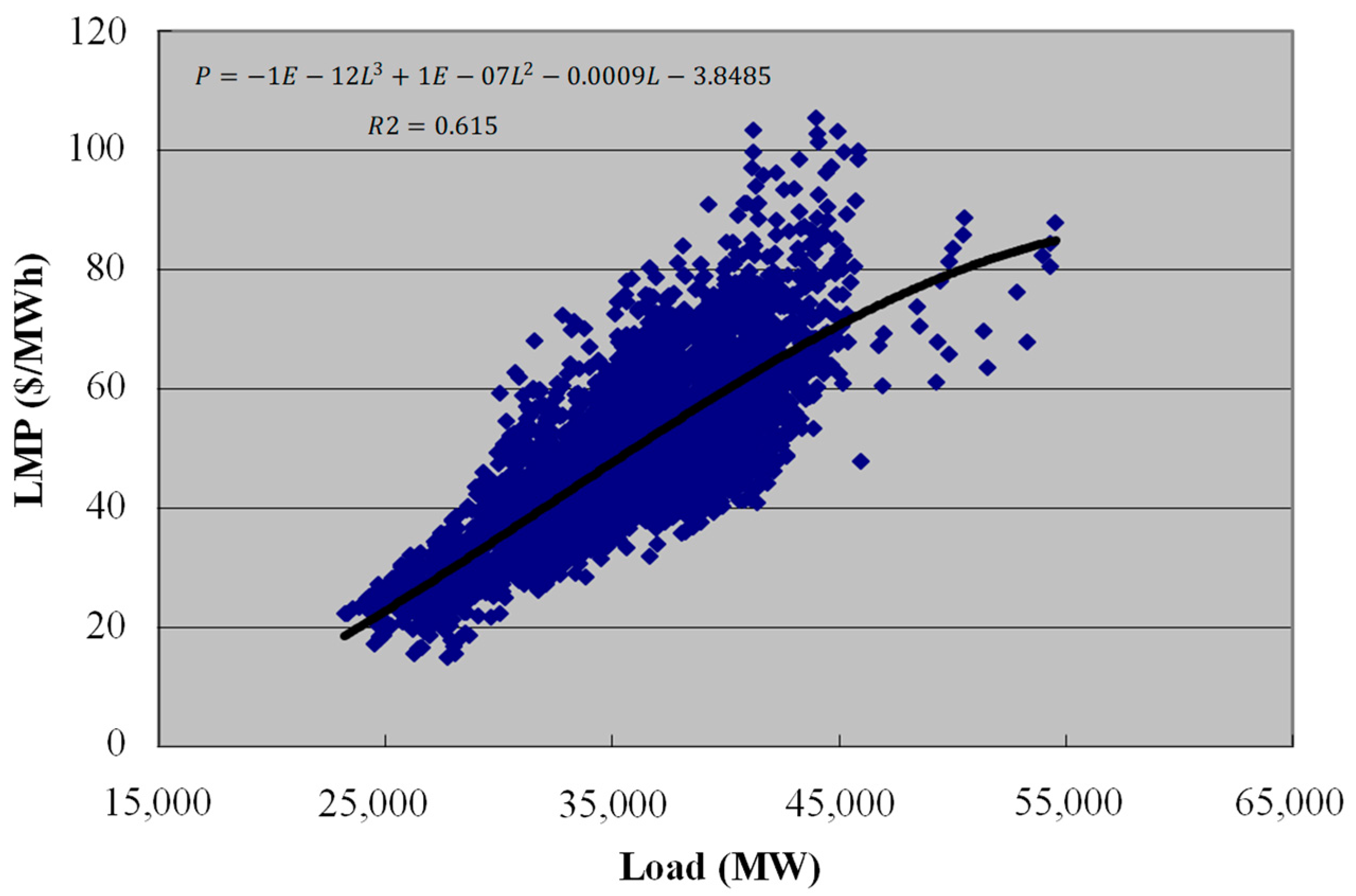
Choosing appropriate data of price and load is important to LMP forecast. We apply the method choosing similar days to increase the performance of the forecasting [19,20]. In the study, the historical data of PJM (Pennsylvania, New Jersey and, Maryland) interchange energy market, including LMP and load were used due to the high degree of reliability and representative. We defined the correlation coefficient () between the price and load in the data, shown as (1). The coefficient of determination is employed to evaluate the correlation. For example, regarding the LMP and load from January to May in 2006, as shown in Figure 1 [10], is 0.615 obtained by the regression simulation, which means the is 0.784 and the LMP and load is high correlation, according to Table 1. Thus, using the load to forecast the LMP is reasonable [21,22,23,24,25].
where
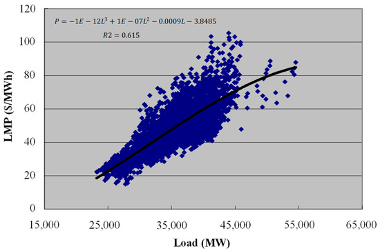
Figure 1.
Relationship between LMP and load in the PJM (January–May 2006).

Table 1.
Related explanation.
is LMP of reference day at number ($/MWh),
is average LMP of reference day ($/MWh),
is load of reference day at number (MW),
is average load reference day (MW).
2.2. Similarity Calculation Model
The purpose of this paper is to forecast LMP according to historical loads and prices, called a day before the forecast day as a reference day. The days which are like the reference day in electricity prices and loads are selected and are namely similar days. The structure of similar days is based on collecting historical data that affect electricity prices and calculate the distance between all historical data and the forecasted day. The correlation between all the data and the forecasted day is evaluated. We adopt four commonly used models in calculating distance, which are Euclidean norm, Manhattan distance, Cosine coefficient and Pearson correlation coefficient. The models with weighted factors are refined, so that obtained model A is the Refined Euclidean norm, model B is the Refined Manhattan distance, mode C is Refined Cosine coefficient, and model D is Refined Pearson correlation coefficient. The models used to evaluate the similarity between the reference days and searched similar days in this paper. Many data science techniques are based on measuring similarity and dissimilarity between objects. Measuring similarity between objects can be performed in a number of ways. Generally, we can divide similarity metrics into two different groups which are similarity-based metrics and distance based metrics. Cosine coefficient and Pearson correlation coefficient are the part of similarity-based metrics and Euclidean distance and Manhattan distance are the part of distance based metrics. We choose those methods because the methods are well-known, relatively easy to use and simple from another method. In our paper, the models of Euclidean distance and Manhattan distance are used to evaluate the data dissimilarity, which means the relativity is higher when the distance value is smaller. The models of Cosine coefficient and Pearson correlation coefficient are used to evaluate the data similarity, which means the relativity is higher when the distance value is bigger. The four refined models are rebuilt as models A, B, C and D, which are described as follows:
2.2.1. Model A: Refined Euclidean Norm
The relativity of Euclidean norm is refined based on [10]. The relativity model involves LMPs and loads of the reference and similar days, shown as (2).
where
- is distance,
- is LMP of reference day at time ($/MWh),
- is LMP of similar day in past at time ($/MWh),
- is load of reference day at time (MW),
- is load of similar day in past at time (MW),
- is LMP of reference day at time ($/MWh),
- is LMP of similar day in past at time ($/MWh),
- is load of reference day at time (MW),
- is load of similar days in past at time (MW),
- is load deviation between reference day and similar days at time (MW),
- is load deviation between reference day and similar days at time (MW),
- is LMP deviation between reference day and similar days at time ($/MWh),
- is LMP deviation between reference day and similar days at time ($/MWh),
- is weight factor
2.2.2. Model B: Refined Manhattan Distance
The relativity of Manhattan distance is refined based on [10]. The relativity model involves LMPs and loads of reference and similar days, shown as (3).
2.2.3. Model C: Refined Cosine Coefficient
The relativity of Cosine coefficient is refined based on [26]. The relativity model involves LMPs and loads of reference and similar days, shown as (4).
where
2.2.4. Model D: Refined Pearson Correlation Coefficient
The relativity of Pearson correlation coefficient is refined based on [26]. The model involves LMPs and loads of reference and similar days, as shown in (5).
where
- is average LMP of reference day at time ($/MWh),
- is average LMP of reference day at time ($/MWh),
- is average LMP of similar day in past at time ($/MWh),
- is average LMP of similar day in past at time ($/MWh),
- is average load of reference day at time (MW),
- is average load of reference day at time (MW),
- is average load of similar day in past at time (MW),
- is average load of similar day in past at time (MW).
The average LMP and load mean the value of the LMP and load as the average values from reference day at time and and also on a similar day in the past at time and .
2.3. Interval of Time Framework
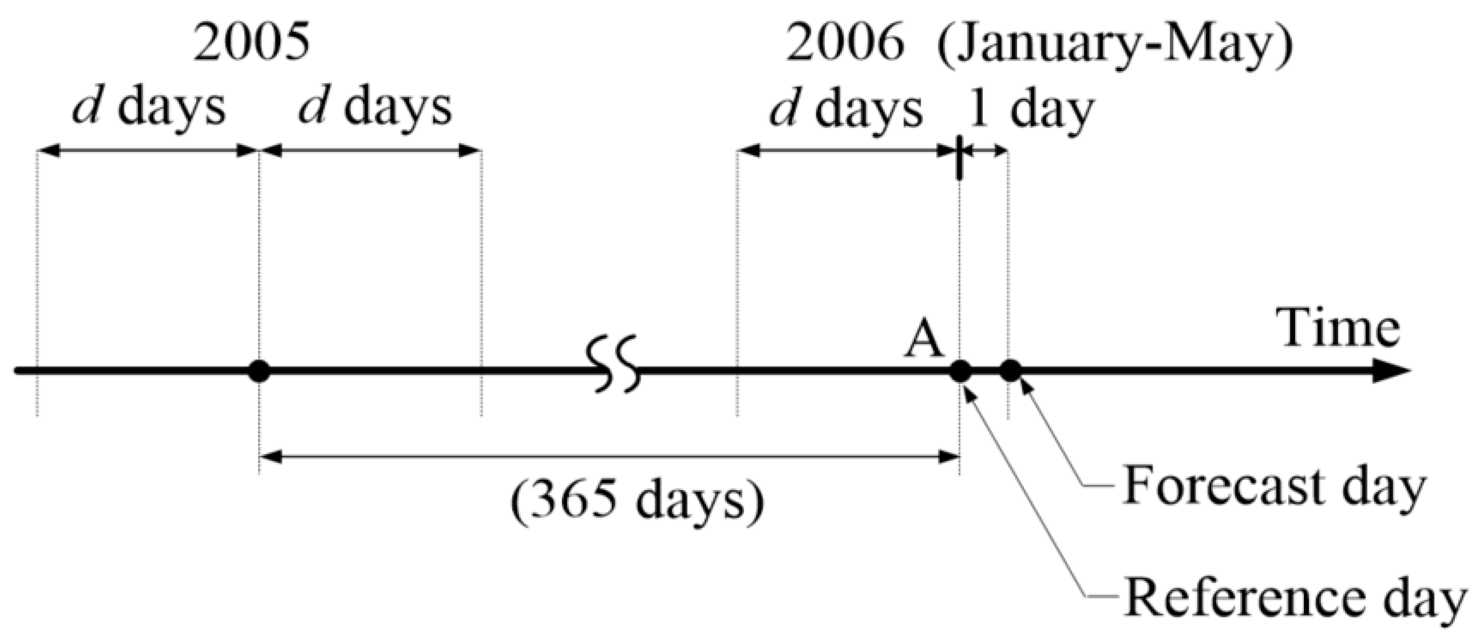
The interval of time framework, d, can be chosen when the reference day is determined, as shown in Figure 2 [26]. For example, assuming that the reference date is point A, the similar days are the d days from the day before a reference day, and past d days before and after the reference day in the previous year. In this study, the d is assumed as 15, 30, 45 and 60.

Figure 2.
Time framework for the selection of similar days.
2.4. Procedure of Similar Date Selection
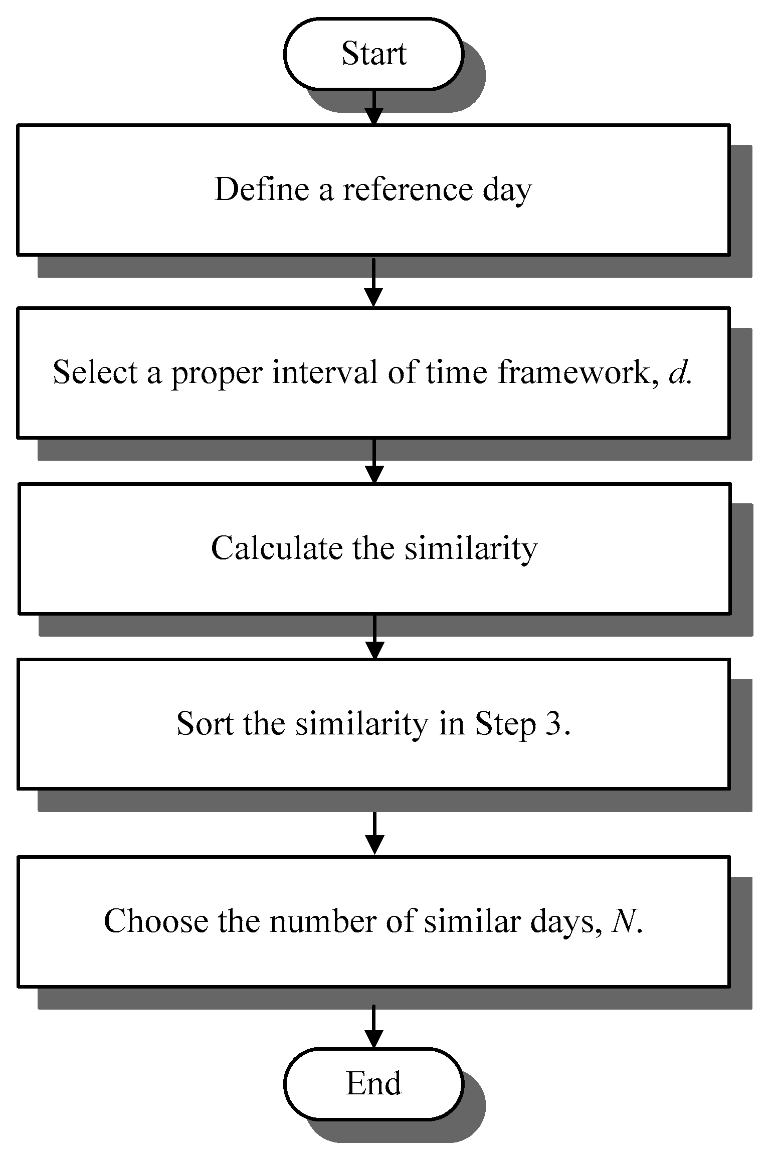
There are five processes to choose similar days which are as follows: reference day definition, interval selection, similarity calculation, similarity sorting, and similar day determination, as shown in Figure 3.
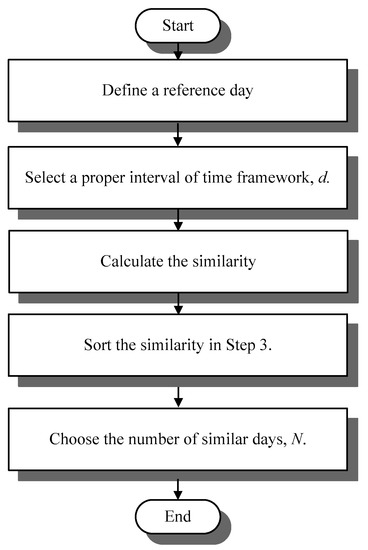
Figure 3.
Similar day selection flowchart.
- Step 1.
- Define a reference day which is one day before the forecasting day;
- Step 2.
- Select a proper interval of time framework, d, based on Figure 2;
- Step 3.
- Equations (2)–(5) are used to calculate the similarity between the selecting days and the reference day in LMP and load;
- Step 4.
- Sort the similarity in Step 3. Note that the (2) and (3) are dissimilarity. Nevertheless (4) and (5) are similarity;
- Step 5.
- Choose the number of similar days, N.
3. Similar Day Regression Model
3.1. Brief Review of Regression Model
The paper uses a typical regression model to forecast the LMPs, as shown in (6), in which the weight factors can be obtained by the least square method [26]. The obtained weight factors in (6) are applied in (2)–(5).
where
is LMP of similar day at time ($/MWh),
is LMP of similar day at time ($/MWh),
is LMP of forecasting day at time ($/MWh),
is load of similar day at time (MW),
is load of similar day at time (MW),
is weight factors .
3.2. Regression Model of Forecasting LMPs
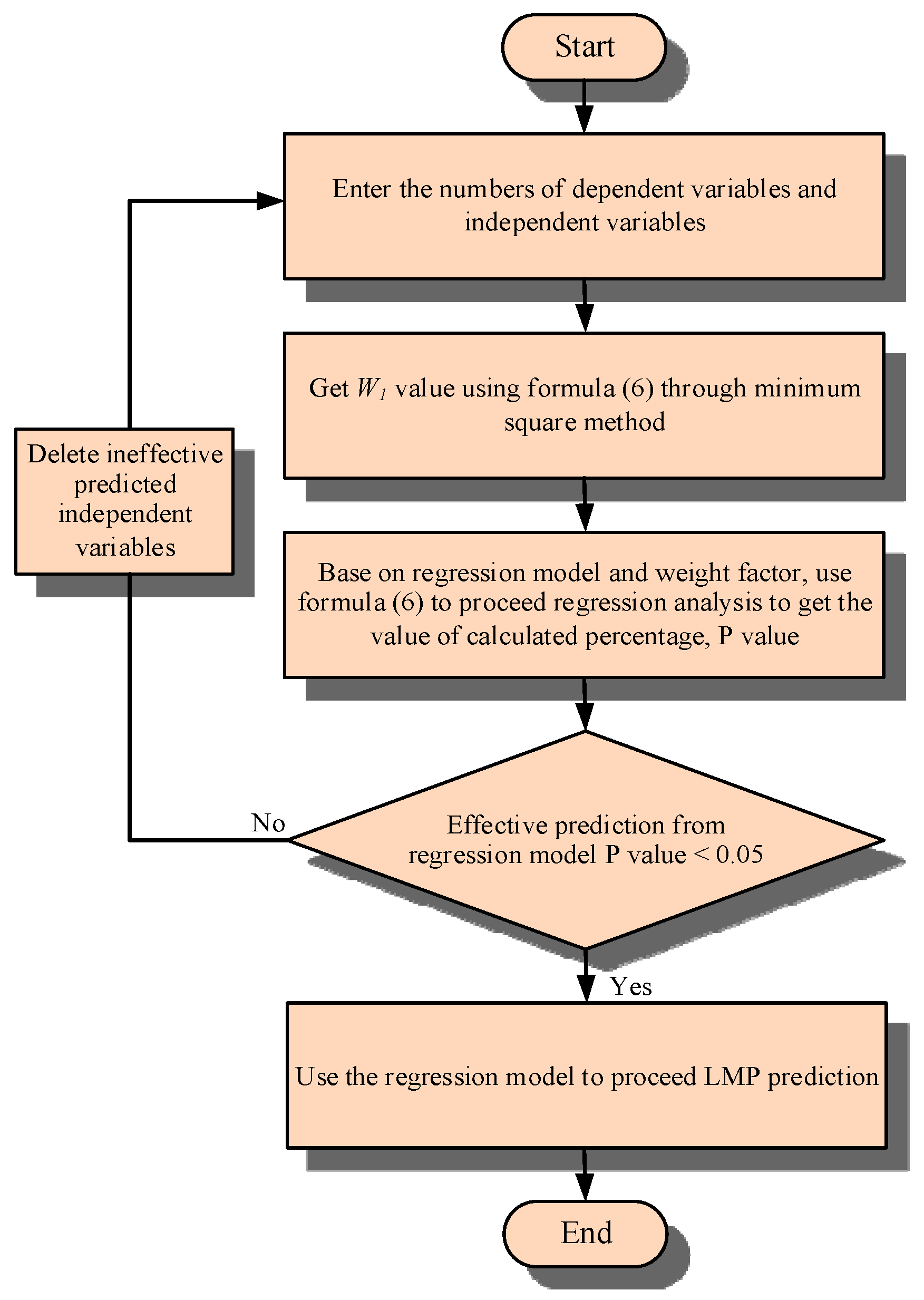
The four steps to forecast LMP by using regression model are variables definition, weight factor analysis, weight factor evaluation, and LMPs forecasting, as shown in Figure 4.
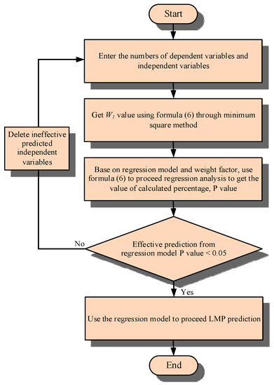
Figure 4.
Regression model forecasting procedure.
- Step 1.
- Variables definition: In the regression model, the dependent variables are assumed as forecasting , and the independent variables are as , , , and ;
- Step 2.
- Weight factor analysis: Base on the LMPs and loads of similar days and the reference day, the weight factors in (6) can be analyzed;
- Step 3.
- Weight factor evaluation: The forecast is acceptable when the probability values (p value) of weight factors are smaller than 0.05. Thus, the independent variables with the P bigger than 0.05 should be removed and the remained weight factors are analyzed though step (2);
- Step 4.
- LMPs forecasting: and in (7) are the average LMP and load data respectively, which are obtained by taking an average of selected N similar days. And the forecasting price can be calculated by the obtained and .
4. Neural Network Based Forecasting Models of Similar Day
4.1. Neural Network Model
Figure 5 illustrates the typical structure of the artificial neural network (ANN) [10] which is consisted of three layers namely input layer, hidden layer, and output layer. The ANN based on price forecasting is called SDANN. The input variables of the proposed SDANN structure for price forecasting are mean similar day data , which is an average of chosen N similar days, actual hourly load , and actual hourly LMP . The output variable of the structure is the LMP of the forecast day, . N is 3, 5, and 10 in this paper.
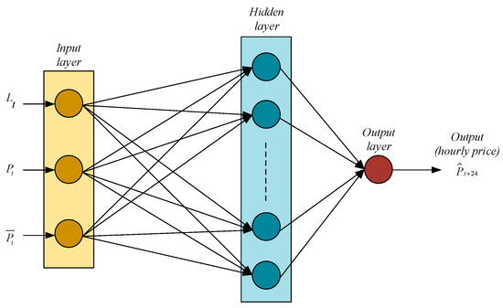
Figure 5.
Neural network architecture diagram.
The applied ANN uses Back-Propagation (BP) algorithm and 2n + 1 hidden neuron is chosen for forecasting where n is the number of input nodes. The weights are adjusted by using the calculated error between forecasting and actual values. The transfer function is sigmoid and relative parameters assumed as the follows: the number of input neurons is 3, the hidden layer is 1, the output neurons is 1, the hidden layer neuron is 7, the learning rate (α) is 0.8, the momentum factor is 0.1 and the iteration is 5000.
4.2. Neural Network Forecasting Model
When using neural network to proceed predicting, firstly, applying neural network proceed LMP forecasting. The historical data which is LMP and load must divide into two section: training data and testing data. Secondly, the training data will be putted into neural network and proceed to repeat training and learning. Finally, the test data will be applied to forecast LMP after finishing training network, as shown in Figure 6 [27].
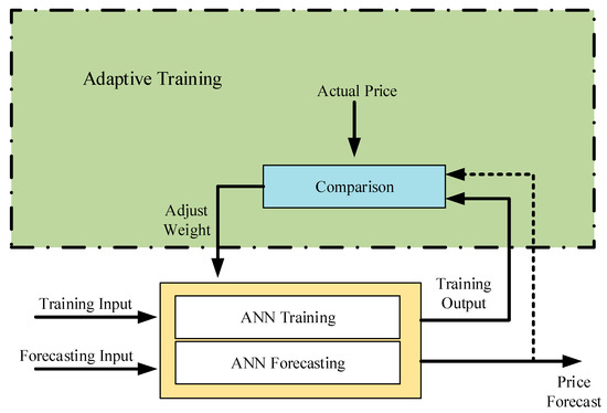
Figure 6.
Price forecast based on neural network.
- (a)
- Training: Selecting similar day interval, d, it is 45 days in the paper, and therefore the load and LMP data have 134 days (excluding the load and LMP of reference day.) as input training data. According to Figure 2, input training data is based on the reference date which is point A. The similar days are the d days from the day before a reference day and past d days before and after the reference day in the previous year. And during training, need to exclude the load and LMP of reference day.
- (b)
- Testing: Forecasting input data is the load and LMP of the reference day.
4.3. Forecast Accuracy
Forecasting prices which are applied to neural network and regression model must examine forecast accuracy by error value. In forecast accuracy, then mean absolute percentage error (MAPE) and forecast mean square error (FMSE) are the standard to verify the accuracy [26].
(a) Mean absolute percentage error
Also known as the absolute average relative error, it can show forecast accuracy accurately, shown as (8):
where
is actual LMP ($/MWh),
is forecasting LMP ($/MWh),
is actual average LMP on prediction day ($/MWh), which is shown in (9).
(b) Forecasting mean square error
The value of FMSE is [0, ∞]. The forecasting accuracy will be lower when the FMSE value is bigger, related to (8) and (9).
The forecasting accuracy will be lower when the FMSE value is bigger, related to (8) and (9).
5. Comparison of Simulation Results
5.1. Regression Model Simulation Result and Comparison
To verify the effectiveness of the proposed method in this research, five days as the forecast days are chosen from the historical data of PJM (Pennsylvania, New Jersey and, Maryland) interchange energy market, which are 20 January, 10 February, 5 March, 7 April and 13 May of 2006. The data used is adequate to be applied in the proposed model. The time choosen as intervals d are 15 days, 30 days, 45 days, and 60 days. We find out similar days N (three days, five days, and 10 days.) through models A to D to be the input of regression model and proceed LMP forecasting. MAPE simulation result of regression model LMP forecasting, which is illustrated in Table 2. To average the simulation result of the 5 forecasting days, obviously, the best LMP forecasting accuracy in model D, d = 45, and N = 3, the MAPE is 9.41%, which is illustrated in Table 3. Therefore, the forecasting performance by using model D to choose similar day is better than the other three models. Moreover, the performance of d = 45 in this research is the best when choosing intervals because there would be problems in cross seasonal electricity using habit differences if the chosen interval is too long. However, if the chosen interval is too short makes the data amount too small. Moreover, the performance is better if similar day, N = 3, because the data chosen is the most like similar day.
Table 2.
Regression model price forecast of MAPE.
Table 3.
Five-day average MAPE analysis (Regression model).
5.2. Neural Network Simulation Result and Comparison
In this study, five days as the forecast days are chosen, which are 20 January, 10 February, 5 March, 7 April and 13 May of 2006. The times chosen as interval d are 15 days, 30 days, 45 days, and 60 days. The similar days N (three days, five days, and 10 days) through models A until D to be the input of the neural network and proceed LMP forecasting. The simulation result is illustrated in Table 4. To average the simulation results of the five forecasting days, obviously, the best forecasting accuracy, which illustrated in Table 5 is from model D (d = 45, N = 3).
Table 4.
Neural network for forecasting electricity price of MAPE.
Table 5.
Five-day average MAPE analysis (Artificial Neural networks).
5.3. Comparison of Regression Forecasting and Neural Network Forecasting
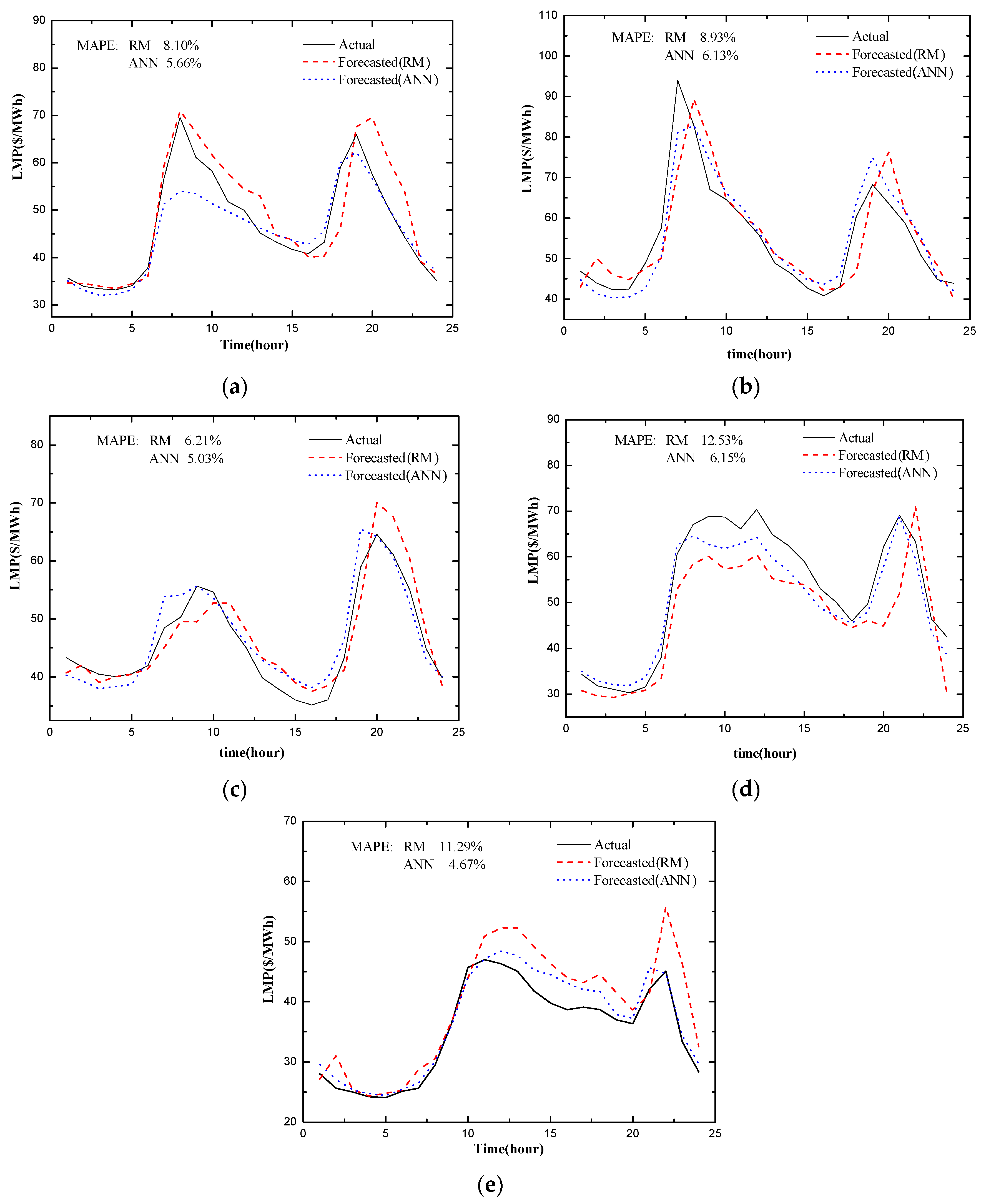
Using model D (with the condition of d = 45 and N = 3), the best forecasting result parameters to proceed the prediction performance comparison by two methods: regression model and neural network (Forecast days are 20 January, 10 February, 5 March, 7 April and 13 May of 2006). The simulation results are illustrated as Figure 7a–e.
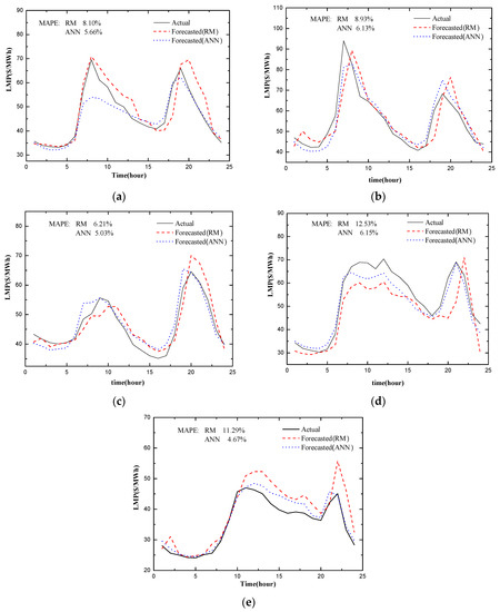
Figure 7.
Results of regression model and neural network forecast price (2006). (a) 20 January, (b) 10 February, (c) 5 March, (d) 7 April, (e) 13 May.
Obviously, from Figure 7, it can be seen that using the neural network to predict location marginal price is closer to actual LMP. The performance using the neural network is better than the regression model forecasting method. The reason is, before predicting, the neural network goes through repeat learning training and the process of error adjustment weight value, whereas regression model lack of the learning character. The MAPE and FMSE of regression model and neural network forecasting price are illustrated in Table 6.
Table 6.
Regression model and neural network forecast price to MAPE and FMSE.
In Table 6, the forecasting accuracy of neural network is better than that of regression model by calculating MAPE and FMSE. Some statistics regarding single forecast day result: For the accuracy of using neural network is minimum 1.18% improved, 6.62% maximum improved, and average forecasting improved is 3.88% in MAPE.
6. Conclusions
This research analyzed and evaluated the four refined mathematical distance models to the application of forecasting short-term electricity prices. Apply the neural network to predict the LMP makes it closer to the actual LMP. Obviously, the performance using the neural network is better than the regression model forecasting method. Moreover, the simulation results show that using the Pearson correlation coefficient model can improve the accuracy of LMP obtained by the regression and neural network models when choosing the time interval of 45 days and similar days of three days.
Author Contributions
Conceptualization, C.-Y.L.; methodology, C.-Y.L.; software, C.-Y.L. and C.-E.W.; validation, C.-Y.L. and C.-E.W.; formal analysis, C.-Y.L. and C.-E.W.; investigation, C.-Y.L.; resources, C.-Y.L. and C.-E.W.; data curation, C.-Y.L.; writing—original draft preparation, C.-Y.L.; writing—review and editing, C.-Y.L.; visualization, C.-Y.L.; supervision, C.-Y.L.; project administration, C.-Y.L.; funding acquisition, C.-Y.L. All authors have read and agreed to the published version of the manuscript.
Funding
This work was supported in part by the Ministry of Science and Technology of Republic of China under Contract MOST 108-2221-E-033-022-MY2.
Conflicts of Interest
The authors declare no conflict of interest.
References
- Chitsaz, H.; Zamani, D.P.; Zareipour, H.; Parikh, P.P. Electricity price forecasting for operational scheduling of behind-the-meter storage systems. IEEE Trans. Smart Grid 2018, 9, 6612–6622. [Google Scholar] [CrossRef]
- Hubicka, K.; Marcjasz, G.; Weron, R. A note on averaging day-ahead electricity price forecasts across calibration windows. IEEE Trans. Sustain. Energy 2019, 10, 321–323. [Google Scholar] [CrossRef]
- Ranjbar, M.; Soleymani, S.; Sadati, N.; Ranjbar, A.M. Electricity price forecasting using artificial neural network. In Proceedings of the 2006 International Conference on Power Electronic, Drives and Energy Systems, New Delhi, India, 12 December 2006; pp. 1–5. [Google Scholar]
- Bissing, D.; Klein, M.T.; Chinnathambi, R.A.; Selvaraj, D.F.; Ranganathan, P. A hybrid regression model for day-ahead energy price forecasting. IEEE Access 2019, 7, 36833–36842. [Google Scholar] [CrossRef]
- Vu, D.H.; Muttaqi, K.M.; Agalgaonkar, A.P.; Bouzerdoum, A. Short-term forecasting of electricity spot prices containing random spikes using a time-varying autoregressive model combined with kernel regression. IEEE Trans. Indus. Inf. 2019, 15, 5378–5388. [Google Scholar] [CrossRef]
- González, C.; McWilliams, M.J.; Juárez, I. Important variable assessment and electricity price forecasting based on regression tree models: Classification and regression trees, bagging and random forests. IET Gener. Trans. Dist. 2015, 9, 1120–1128. [Google Scholar] [CrossRef]
- Pourdaryaei, A.; Mokhlis, H.; Illias, H.A.; Kaboli, S.H.A.; Ahmad, S.; Ang, S.P. Hybrid ANN and artificial cooperative search algorithm to forecast short-term electricity price in de-regulated electricity market. IEEE Access 2019, 7, 125369–125386. [Google Scholar] [CrossRef]
- Alanis, A.Y. Electricity prices forecasting using artificial neural networks. IEEE Lat. Am. Trans. 2018, 16, 105–111. [Google Scholar] [CrossRef]
- Mosbah, H.; El-hawary, M. Hourly electricity price forecasting for the next month using multilayer neural network. Can. J. Elect. Comp. Eng. 2016, 39, 283–291. [Google Scholar] [CrossRef]
- Voronin, S.; Partanen, J.; Kauranne, T. A hybrid electricity price forecasting model for the Nordic electricity spot market. Int. Trans. Elec. Energy Syst. 2014, 24, 736–760. [Google Scholar] [CrossRef]
- Lee, C.Y.; Tuegeh, M. Optimal optimisation-based microgrid scheduling considering impacts of unexpected forecast errors due to the uncertainty of renewable generation and loads fluctuation. IET Renew. Power Gen. 2020, 14, 321–331. [Google Scholar] [CrossRef]
- Lee, C.Y.; Tuegeh, M. An optimal solution for smooth and non-smooth cost functions-based economic dispatch problem. Energies 2020, 13, 3721. [Google Scholar] [CrossRef]
- Shrivastava, N.A.; Khosravi, A.; Panigrahi, B.K. Prediction interval estimation of electricity prices using PSO-tuned support vector machines. IEEE Trans. Ind. Inf. 2015, 11, 322–331. [Google Scholar] [CrossRef]
- Peesapati, R.; Kumar, N. Electricity price forecasting and classification through wavelet–dynamic weighted PSO–FFNN approach. IEEE Syst. J. 2017, 12, 3075–3084. [Google Scholar]
- Pourdaryaei, A.; Mokhlis, H.; Illias, H.A.; Kaboli, S.H.A.; Ahmad, S. Short-term electricity price forecasting via hybrid backtracking search algorithm and ANFIS approach. IEEE Access 2019, 7, 77674–77691. [Google Scholar] [CrossRef]
- Darudi, A.; Bashari, M.; Javidi, M.H. Electricity price forecasting using a new data fusion algorithm. IET Gener. Trans. Distr. 2015, 9, 1382–1390. [Google Scholar] [CrossRef]
- González, J.P.; Muñoz San Roque, A.M.S.; Pérez, E.A. Forecasting functional time series with a new hilbertian armax model: Application to electricity price forecasting. IEEE Trans. Power Syst. 2018, 33, 545–556. [Google Scholar] [CrossRef]
- Bello, A.; Bunn, D.W.; Reneses, J.; Muñoz, A. Medium-term probabilistic forecasting of electricity prices: A hybrid approach. IEEE Trans. Power Syst. 2017, 32, 334–343. [Google Scholar] [CrossRef]
- Khosravi, A.; Nahavandi, S.; Creighton, D. Quantifying uncertainties of neural network-based electricity price forecasts. Appl. Energy 2013, 112, 120–129. [Google Scholar] [CrossRef]
- Chang, P.C.; Fan, C.Y.; Lin, J.J. Monthly electricity demand forecasting based on a weighted evolving fuzzy neural network approach. Int. J. Elect. Power Energy Syst. 2011, 33, 17–27. [Google Scholar] [CrossRef]
- Esmaili, M.; Shayanfar, H.A.; Moslemi, R. Locating series FACTS devices for multi-objective congestion management improving voltage and transient stability. Eur. J. Oper. Res. 2014, 236, 763–773. [Google Scholar] [CrossRef]
- Bharatwaj, N.V.; Abhyankar, A.R.; Bijwe, P.R. Improved loss distribution and modeling in DCOPF. Int. J. Elec. Power Energy Syst. 2013, 53, 416–425. [Google Scholar] [CrossRef]
- Sarkar, V.; Khaparde, S.A. Reactive power constrained OPF scheduling with 2-d locational marginal pricing. IEEE Trans. Power Syst. 2013, 28, 503–512. [Google Scholar] [CrossRef]
- Lewis, G. Estimating the value of wind energy using electricity locational marginal price. Energy Policy 2010, 38, 3221–3231. [Google Scholar] [CrossRef]
- Gautam, D.; Mithulananthan, N. Locating distributed generator in the LMP-based electricity market for social welfare maximization. Electr. Power Compon. Syst. 2007, 35, 489–503. [Google Scholar] [CrossRef]
- Nozawa, T.; Konda, M.; Fujibayashi, M.; Imai, M.; Kotani, K.; Sugawa, S.; Ohmi, T. A parallel vector-quantization processor eliminating redundant calculations for real-time motion picture compression. IEEE J. Solid State Circuits 2000, 35, 1744–1751. [Google Scholar] [CrossRef]
- Bastian, J.; Zhu, J.X.; Banunarayanan, V.; Mukerji, R. Forecasting energy prices in a competitive market. IEEE Comp. Appl. Power 1999, 12, 40–45. [Google Scholar] [CrossRef]


© 2020 by the authors. Licensee MDPI, Basel, Switzerland. This article is an open access article distributed under the terms and conditions of the Creative Commons Attribution (CC BY) license (http://creativecommons.org/licenses/by/4.0/).