Optimized Layouts of Borehole Thermal Energy Storage Systems in 4th Generation Grids

Abstract

Borehole thermal energy storage (BTES) systems are a viable option to meet the increasing cooling demand and to increase the sustainability of low-temperature district heating and cooling (DHC) grids. They are able to store the rejected heat of cooling cycles on a seasonal basis and deliver this heat during the heating season. However, their efficient practical implementation requires a thorough analysis from technical, economic and environmental points of view. In this comparative study, a dynamic exergoeconomic assessment is adopted to evaluate various options for integrating such a storage system into 4th generation DHC grids in heating dominated regions. For this purpose, different layouts are modeled and parameterized. Multi-objective optimization is conducted, varying the most important design variables in order to maximize exergetic efficiency and to minimize levelized cost of energy (LCOE). A comparison of the optimal designs of the different layouts reveals that passive cooling together with maximizing the heating temperature shift, accomplished by a heat pump, lead to optimal designs. Component-wise exergy and cost analysis of the most efficient designs highlights that heat pumps are responsible for the highest share in inefficiency while the installation of BTES has a high impact in the LCOE. BTES and buffer storage tanks have the lowest exergy destruction for all layouts and increasing the BTES volume results in more efficient DHC grids.

1. Introduction

In European households, heating accounts for 78% of the total final energy use. Cooling of buildings still has a fairly small share in the energy use, but the demand during summer months is continuously rising due to climate change [1]. It is estimated that by 2025 the installed cooling capacity in Europe is likely to be 55–60% higher than in 2010 [2]. Therefore, simultaneous supply of heating and cooling needs to be considered as an important part of the future energy supply system.

By 2050, more than 80% of European residents are expected to live in urban areas [3]. This trend increases the benefits of district energy systems, which tend to be more economic for densely populated regions [4]. District heating and cooling (DHC) systems can be environmentally beneficial and pave the way toward the sustainable energy supply, if they are applied appropriately [4,5].

The 4th generation district heating (DH) concept specifies some prerequisites that need to be met for the proper application of DH systems and the fulfillment of their role in a future sustainable energy economy. The most important ones are the implementation of low-temperature DH networks, the ability to recycle heat from low-temperature sources such as solar and geothermal heat and the implementation as an integrated part of smart energy systems [6]. A future 4th generation district cooling (DC) system can be defined as a system more interactive with the electricity, DH and gas grids [6]. Overall, a 4th generation DHC grid can be considered as a low-temperature interactive energy grid for supplying heating and cooling demands.

Every cooling process involves the rejection of excess heat to a heat sink. Lower sink temperatures generally result in a more efficient system operation. As the temperature of the ground during cooling seasons is lower and more stable than the ambient temperature, it can be used as an efficient heat sink by utilizing borehole heat exchangers (BHEs). In addition, arrays of BHEs are suitable thermal energy storage systems for waste heat and fluctuating renewable energy sources [7]. Such borehole thermal energy storage (BTES) systems exploit the high heat capacity of the underground to store large quantities of heat on a seasonal basis in the geological environment [8]. The results of analyzing the influence of design parameters on energetic performance of medium deep BTES systems showed that they can have a very high efficiency of more than 80% in large-scale applications [7,9,10,11].

Aforementioned benefits of BTES systems and the increasing trend of installing cooling capacity in Europe, makes the utilization of BTES-assisted 4th generation DHC grids an interesting concept for future energy supply. These benefits have been already proven by several projects (e.g., [12,13,14]). A review of some of these projects can be found in [15]. However, there are not enough guidelines for designing BTES systems in DHC grids. An efficient implementation of this concept requires more detailed assessments and system design from technical, economic and environmental points of view. A BTES should not be regarded in isolation, but merely as one component within a district heating and cooling network [8,16,17]. Therefore, a method needs to be selected that evaluates the optimal integration of BTES systems into DHC grids considering their interaction with other components.

An energy carrier’s exergy is defined by its potential to interact with its environment [18], namely the availability of energy. Exergoeconomics is the branch of engineering that combines exergy analysis and economic principles. It can provide information to a system designer which are not available through conventional energy analysis and economic evaluations, but crucial to the design and operation of a cost-effective system [18]. Moreover, increasing exergy efficiency leads to reduced environmental impacts and a higher sustainability [19]. For environmental evaluation of BTES and energy systems, Life Cycle Assessment (LCA) has been proven to be a useful tool [20,21]. However, LCA lacks thermodynamic assessment [19]. Therefore, the exergoeconomic analysis method can be considered as a method which takes technical, economic and environmental aspects into consideration. Moreover, by adding CO₂ emission costs to the total costs, economic effects of direct environmental emissions can be considered as well.

Exergy analysis of an installed BTES system for heating and cooling applications was done by Kizilkan and Dincer [22,23]. These studies specify that a significant energy saving can be done by determining the exergy destruction of the whole system and its components. However, they have mainly used a static approach, which is suitable for high-temperature systems., e.g., power generation systems. When a system’s operating temperature is close to the reference state, e.g., heating and cooling systems, the utilization of a dynamic approach is necessary [24].

In this study, a dynamic exergoeconomic assessment approach including CO₂ emission costs is adapted to BTES systems to render a comprehensive technical, economic and environmental assessment of their implementation into 4th generation DHC grids. The approach is presented on the example of a generic case study. After giving a general overview on this case study, different system layouts and scenarios are specified. Moreover, mathematical optimization is done for each scenario using the outputs of the exergoeconomic assessment approach as objective functions, varying the most sensitive system parameters. Finally, the results are compared and discussed.

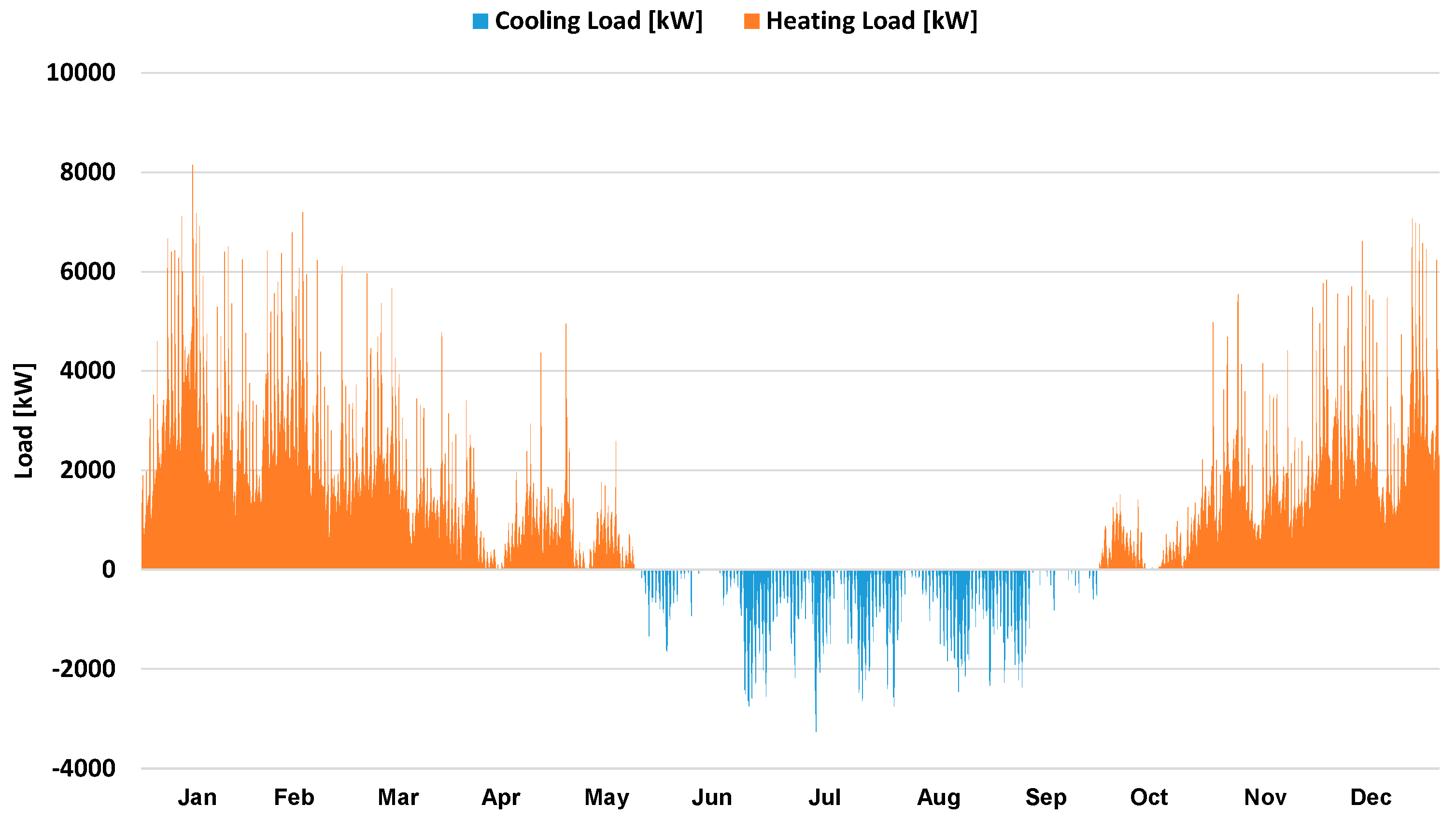
2. Case Study Setup

For the case study, a notional district located in Frankfurt, Germany is chosen. Frankfurt is located in a heating-dominated region with a low cooling demand, which is mainly caused from the commercial and industrial sectors. It is assumed to consist of 100 single family houses, 100 multifamily houses and 50 office buildings. After designing 3D thermal zone models of each building type, load profiles are calculated in TRNBuild [25]. Boundary conditions are based on standard libraries for building construction types of renovated buildings [26], schedules (e.g., occupation) [27] and regime types (e.g., heating and cooling set point temperature) [27]. The weather data from Frankfurt airport is taken from Meteonorm data [28].

Figure 1 shows the calculated load profile. The total annual heating and cooling demands of the DHC grid are 8.47 GWh and 1.05 GWh, respectively, with more than 70% of the cooling demand for the office buildings. Supply and return temperatures (T_sup, T_ret) of the grid are 6 °C and 12 °C for active and 18 °C and 22 °C for passive cooling. In accordance to the 4th generation DH concept, supply and return temperatures are set to 45 °C and 35 °C during the heating season [29].

3. System Design Scenarios

Four generally different designs of the case district’s heating and cooling system shall be evaluated. The proposed scenarios are summarized in

Table 1. The proposed scenarios.

Scenario	Cooling	GB	HPs	BST
ActSer	Active	Serial	Single stage	Cooling/Heating
ActPar	Active	Parallel	Double stage	Cooling/Heating
PasSer	Passive	Serial	Single stage	Cooling/Heating
PasPar	Passive	Parallel	Double stage	Cooling/Heating

. All scenarios comprise a BTES system which is discharged by a heat pump (HP). Furthermore, the systems contain one or two gas boilers (GB) to cover heat demands which are not covered by the BTES system. Moreover, all scenarios include a buffer storage tank (BST) which is needed to lower the size of the BTES system, to maximize the total load supply from the ground loop and to operate the HPs more steadily by smoothening the load demands. The four scenarios generally differ by their approach of cooling (active or passive) and by the connection of the BTES system and the GB (serial or parallel). All four systems have their own characteristics during heating and cooling operation, respectively, which shall be outlined in the following.

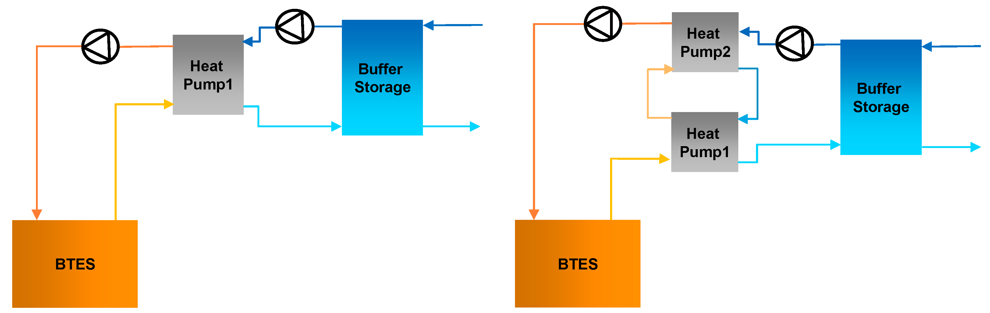
3.1. Cooling Operation

The DHC is located in a heating-dominated region. The two general cooling approaches are

• Active Cooling (Scenarios ActSer and ActPar): The total cooling load is supplied actively by heat pumps, which use the BTES as their heat sink (Figure 2) and
• Passive Cooling (Scenarios PasSer and PasPar): The total cooling load is supplied passively by the BTES using heat exchangers (HEX), which separate load and sink side (Figure 3).

The BTES temperature difference is taken as 5 K for active and 3 K for passive scenarios. The nominal BTES side flow rate of the HP, as well as the connected pump, are specified accordingly and at a BTES side temperature of 15 °C. The pump is turned on or off by a thermostat, which monitors the BST supply temperature.

In the active scenarios, either a single stage HP covers the whole cooling demand (ActSer), or each double stage HP module covers it partially (ActPar). Double stage HPs are selected for ActPar scenario, because of their more efficient operation in partial cooling mode. The nominal load side flow rate of the HP, as well as that of the connected pump, are selected according to the design supply and return temperatures. The BST thermostat turns on or off the pump and its flow rate is regulated considering the HP output capacity. For passive scenarios, the same on/off strategy operates the pump and the regulation is done considering the energy balance equation of the HEX.

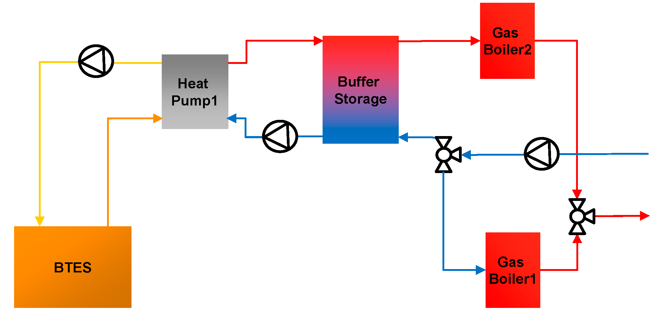
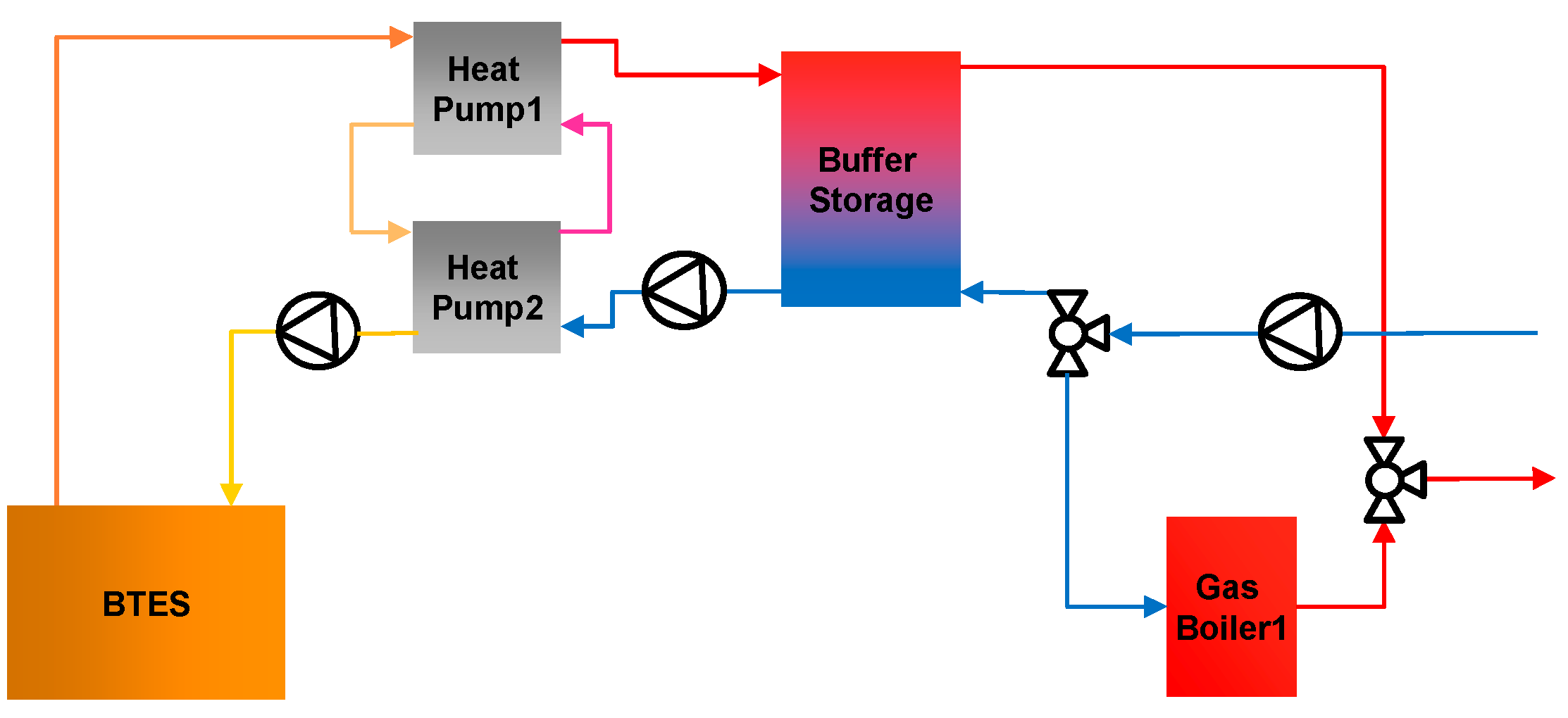
3.2. Heating Operation

The scenarios in heating mode are defined to compare the effect of the temperature shift and the maximum corresponding heating load that can be supplied efficiently by the ground loop. The design temperature difference of the BTES for heating mode is suggested to be between 3–5 K by some geothermal HP manufacturers [30]. In some practical applications this is taken as approx. 4 K [14,31]. 4 K can hardly be achieved for serially-connected HPs at full load performance (according to the manufacturer’s data [32]). Therefore, to have similar boundary conditions for all scenarios, it is taken as 5 K for this study. The nominal flow rate of the HP on the source side and the connected pump are specified to meet the temperature difference at a source side temperature of 10 °C. The pump is controlled by the BST on/off thermostat. On the load side, lower temperature shifts increase the COP of the HP but result in a lower BST efficiency [33] and a higher power consumption of the circulating pumps. Consequently, the serial and parallel scenarios are proposed to assess partial and full grid temperature shift by the ground loop, respectively. Like active cooling scenarios, the load side pump is turned on or off by the BST thermostat and its flow rate is regulated considering the HP output capacity.

3.2.1. Serial Scenarios

In serial mode (Figure 4) the HP consists of single stage modules, which heat the return water temperature from the bottom of the BST up to a specific set point temperature. The supplementary boiler GB2, which is connected to the BST in series, provides the additional heat up to the grid supply temperature of 45 °C. The maximum volume flow rate from the grid, which is sent from the diverter to the BST, is specified regarding the selected HP capacity for its continuous daily operation during the peak heating day. On the load side, the overall heat pump capacity (${\mathrm{Cap}}_{\mathrm{HP}}$), the temperature shift of the BST ($\Delta {\mathrm{T}}_{\mathrm{BST}}$) and the volume of the BST (${\mathrm{Vol}}_{\mathrm{BST}}$) are selected using an optimization approach. Consequently, as the case study is located in a heating-dominated region, GB1 supplies the rest of the overall heating demand, which cannot be supplied by the HP and GB2 optimally.

3.2.2. Parallel Scenarios

The system layout for parallel scenarios is shown in Figure 5. Two serially-connected HPs heat the return fluid from the BST up to the grid supply temperature. The amount of heat which cannot be supplied by the ground loop will be supplied by the gas boiler, which is in parallel operation with the HPs. On the load side, the maximum amount of the return fluid which is sent to the BST, ${\mathrm{Cap}}_{\mathrm{HP}}$ and ${\mathrm{Vol}}_{\mathrm{BST}}$ are specified with the same strategy as the serial scenario and $\Delta {\mathrm{T}}_{\mathrm{BST}}$ is fixed to the grid temperature shift.

A reference scenario is designed based on energetically-efficient conventional systems. In this reference case, the total heating demand is supplied by condensing GBs with a high energetic efficiency of 95% [34] and the whole cooling demand is covered by air-source HPs with a seasonal COP of 4 [35].

4. Evaluation Criterion

4.1. Exergy Analysis

As mentioned earlier, exergy is defined as a system’s potential to interact with its environment. For thermal systems, this corresponds to the temperature difference between the heat carrier medium and a predefined reference temperature. A variation of the reference temperature does not affect the results of an exergy analysis significantly for systems with higher operating temperatures (e.g., power plants). In contrast, when operation temperatures of a system are close to the reference temperature (e.g., in heating and cooling systems), the results of an exergy analysis strongly depends on the definition of the reference environment [36]. The reference temperature for a steady-state exergy analysis must be chosen as a fixed temperature, such as the seasonal mean temperature or annual mean temperature. For the dynamic analysis, however, several possible reference temperatures like the indoor air temperature, the undisturbed ground temperature and the outdoor temperature are discussed [36]. In this study, the outdoor temperature is considered as the reference temperature. Thermal exergy of a fluid, which can be used for exergy calculations in heating and cooling systems [24], can be calculated using Equation (1). ${\mathrm{T}}_0$ is the reference temperature and is taken as the ambient temperature in this study.

$$\stackrel{·}{\mathrm{E}}={\stackrel{·}{\mathrm{m}}\mathrm{c}}_{\mathrm{p}}\times (\left(\mathrm{T}-{\mathrm{T}}_0\right)-{\mathrm{T}}_0\ln \frac{\mathrm{T}}{{\mathrm{T}}_0})$$

(1)

The exergetic efficiency (${\mathsf{\eta }}_{\mathrm{exergy}}$) of a system is the ratio of the output exergy rate (${\stackrel{·}{\mathrm{E}}}_{\mathrm{out}}$) to the exergy rate of the expended resources (${\stackrel{·}{\mathrm{E}}}_{\mathrm{in}}$) to generate this output. By integrating ${\stackrel{·}{\mathrm{E}}}_{\mathrm{in}}$ and ${\stackrel{·}{\mathrm{E}}}_{\mathrm{out}}$ into each time step over a system’s lifetime (${\mathrm{n}}_{\mathrm{end}}$), its overall average ${\mathsf{\eta }}_{\mathrm{exergy}}$ can be calculated (Equation (2)).

$${\mathsf{\eta }}_{\mathrm{exergy}}=\frac{{\sum }_{\mathrm{n}=0}^{{\mathrm{n}}_{\mathrm{end}}}{\stackrel{·}{\mathrm{E}}}_{\mathrm{out},\mathrm{n}}}{{\sum }_{\mathrm{n}=0}^{{\mathrm{n}}_{\mathrm{end}}}{\stackrel{·}{\mathrm{E}}}_{\mathrm{in},\mathrm{n}}}\times 100\%$$

(2)

Dynamic exergy calculation of ${\stackrel{·}{\mathrm{E}}}_{\mathrm{out}}$ and ${\stackrel{·}{\mathrm{E}}}_{\mathrm{in}}$ for the whole system in heating load (HL) and cooling load (CL) supply can be calculated using Equations (3) and (4), respectively.

$$\begin{gathered} {\stackrel{·}{\mathrm{E}}}_{\mathrm{out},\mathrm{HL}}=\{\begin{array}{c}{\stackrel{·}{\mathrm{E}}}_{\mathrm{sply}}-{\stackrel{·}{\mathrm{E}}}_{\mathrm{rtn}} {\mathrm{T}}_0\le {\mathrm{T}}_{\mathrm{ret}} \\ {\stackrel{·}{\mathrm{E}}}_{\mathrm{sply}} {\mathrm{T}}_{\mathrm{ret}}<{\mathrm{T}}_0\le {\mathrm{T}}_{\sup } \\ 0 {\mathrm{T}}_0\ge {\mathrm{T}}_{\sup }\end{array} \\ {\stackrel{·}{\mathrm{E}}}_{\mathrm{in},\mathrm{HL}}={\stackrel{·}{\mathrm{E}}}_{\mathrm{elec}}+{\stackrel{·}{\mathrm{E}}}_{\mathrm{gas}}+{\stackrel{·}{\mathrm{E}}}_{\mathrm{BTES}} \end{gathered}$$

(3)

$$\begin{gathered} {\stackrel{·}{\mathrm{E}}}_{\mathrm{out},\mathrm{CL}}=\{\begin{array}{c}{\stackrel{·}{\mathrm{E}}}_{\sup }-{\stackrel{·}{\mathrm{E}}}_{\mathrm{ret}} {\mathrm{T}}_0\ge {\mathrm{T}}_{\mathrm{ret}} \\ {\stackrel{·}{\mathrm{E}}}_{\sup } {\mathrm{T}}_{\sup }\le {\mathrm{T}}_0<{\mathrm{T}}_{\mathrm{ret}} \\ 0 {\mathrm{T}}_0\le {\mathrm{T}}_{\sup }\end{array} \\ {\stackrel{·}{\mathrm{E}}}_{\mathrm{in},\mathrm{CL}}={\stackrel{·}{\mathrm{E}}}_{\mathrm{elec}}+{\stackrel{·}{\mathrm{E}}}_{\mathrm{gas}}-{\stackrel{·}{\mathrm{E}}}_{\mathrm{BTES}} \end{gathered}$$

(4)

where ${\stackrel{·}{\mathrm{E}}}_{\mathrm{BTES}}$ is the exergy which is stored in or extracted from the BTES system during heating and cooling seasons, it can be calculate using Equation (5). ${\mathrm{T}}_{\mathrm{b}}$ denotes the temperature on the boundary where heat transfer (${\stackrel{\text{·}}{\mathrm{Q}}}_{\mathrm{BTES}}$) occurs [9]. As BTES is considered as a component in the DHC grid, it is taken as the average storage temperature.

$${\stackrel{·}{\mathrm{E}}}_{\mathrm{BTES}}={\stackrel{\text{·}}{\mathrm{Q}}}_{\mathrm{BTES}}\times (1-\frac{{\mathrm{T}}_0}{{\mathrm{T}}_{\mathrm{b}}})$$

(5)

${\stackrel{·}{\mathrm{E}}}_{\mathrm{gas}}$, the chemical exergy of natural gas, can be calculated by Equation (6) [37] using the lower heating value (LHV) of natural gas.

$${\stackrel{·}{\mathrm{E}}}_{\mathrm{gas}}\approx 1.04\times \mathrm{LHV}$$

(6)

4.2. Economic Analysis

The total expenditures to generate the output consists of capital investment costs (${\stackrel{\text{·}}{\mathrm{C}}}_{\mathrm{IC}}$), maintenance costs (${\stackrel{\text{·}}{\mathrm{C}}}_{\mathrm{MC}}$), fuel costs (${\stackrel{\text{·}}{\mathrm{C}}}_{\mathrm{f}}$) and environmental costs (${\stackrel{\text{·}}{\mathrm{C}}}_{\mathrm{env}}$). By dividing the net present value of the total cost by the discounted total energy output, levelized cost of energy ($\mathrm{LCOE}$) can be calculated using Equation (7) [38]. The system lifetime $\left({\mathrm{n}}_{\mathrm{end}}\right)$ and the discount rate ($\mathrm{i}$) are assumed to be 30 years and 3%, respectively.

$$\mathrm{LCOE}=\frac{{\sum }_{\mathrm{n}=0}^{{\mathrm{n}}_{\mathrm{end}}}({{\stackrel{·}{\mathrm{C}}}_{\mathrm{IC},\mathrm{n}}+{\stackrel{·}{\mathrm{C}}}_{\mathrm{MC},\mathrm{n}}+{\stackrel{·}{\mathrm{C}}}_{\mathrm{f},\mathrm{n}}+{\stackrel{·}{\mathrm{C}}}_{\mathrm{env},\mathrm{n}})\cdot (1+\mathrm{i})}^{-\mathrm{n}}}{{\sum }_{\mathrm{n}=0}^{{\mathrm{n}}_{\mathrm{end}}}{\stackrel{·}{\mathrm{Q}}}_{\mathrm{out},\mathrm{n}}{\left(1+\mathrm{i}\right)}^{-\mathrm{n}}}\times 100\%$$

(7)

Investment cost (IC) and maintenance cost (MC) functions of the main components are listed in

Table 2. Cost function of different components.

Component	Investment Cost Function (€)	Maintenance (€/yr.)	Reference
BTES	65 × LBHE	-	[39]
Property	75.05 × AProperty	-	[40]
HP	(2053.8·CapHP−0.348) × CapHP	0.0075 × CIC	[41]
BST	(130 + 11,680·VolBST−0.5545) × VolBST	-	[42]
GB	(11,418.60 + 64.6115·CapGB0.7978) × fGB a	0.02 × CIC	[43]

^a f_GB = 1.0818 − 8.2898·10⁻⁷ Cap_GB.

. After summing up electricity consumptions (${\mathrm{f}}_{\mathrm{elec}}$) as well as gas consumptions (${\mathrm{f}}_{\mathrm{gas}}$) in each time step over the system lifetime for each simulation, fuel and environmental costs are calculated using Equations (8) and (9). Electricity and gas costs (${\mathrm{c}}_{\mathrm{elec}}$ and ${\mathrm{c}}_{\mathrm{gas}}$), Global Warming Potential as a result of the consumption of electricity and gas (${\mathrm{GWP}}_{\mathrm{elec}}$ and ${\mathrm{GWP}}_{\mathrm{gas}}$) and the emission costs (${\mathrm{c}}_{\mathrm{CO}2}$) as a function of the assessment year are calculated as given in

Table 3. Fuel costs, CO2 costs and GWP.

Parameter	Cost Function 2020–2030	Cost Function 2030–2050	Reference
Celec,n(€/kWh)	0.002364n + 0.131	−0.0005n + 0.1625	[44,45]
Cgas,n(€/kWh)	0.00216n + 0.0268	0.00321n + 0.04702	[44,45]
cCO2,n(€/tCO2)	−0.2083n2 + 9.072n + 5.553	80	[46]
GWPelec,n(tCO2/kWh)	(−20.99n + 423.89) × 10−6	(−8.595n + 287.55) × 10−6	[47]
GWPgas,n(tCO2/kWh)	250 × 10−6	250 × 10−6	[48]

.

$${\stackrel{\text{·}}{\mathrm{C}}}_{\mathrm{f},\mathrm{n}}={\mathrm{f}}_{\mathrm{elec},\mathrm{n}}{\mathrm{c}}_{\mathrm{elec},\mathrm{n}}+{\mathrm{f}}_{\mathrm{gas},\mathrm{n}}{\mathrm{c}}_{\mathrm{gas},\mathrm{n}}$$

(8)

$${\stackrel{\text{·}}{\mathrm{C}}}_{\mathrm{env},\mathrm{n}}={\mathrm{f}}_{\mathrm{elec},\mathrm{n}}{\mathrm{c}}_{\mathrm{CO}2,\mathrm{n}}{\mathrm{GWP}}_{\mathrm{elec},\mathrm{n}}+{\mathrm{f}}_{\mathrm{gas},\mathrm{n}}{\mathrm{c}}_{\mathrm{CO}2,\mathrm{n}}{\mathrm{GWP}}_{\mathrm{gas},\mathrm{n}}$$

(9)

4.3. Exergoeconomic Analysis

In every technoeconomic evaluation, the aim is to minimize cost and to maximize the efficiency. Therefore, the two objective functions, Equations (2) and (7), need to be optimized simultaneously. Setup and boundaries of the optimization variables and technical constraints are summarized in

Table 4. Ranges of optimization variables and constraints.

Subject to	Reason
30 m ≤ LBHE ≤ 400 m	Length range of shallow BHEs [49]
30 ≤ NBHE ≤ 1200	Heat transfer range of BHEs (W/m), corresponds to LBHE
2 m ≤ SBHE ≤ 25 m	Maximum available surface area
50 kW ≤ CapHP ≤ 8150 kW	Minimum capacity of each HP module/Maximum heating load
25 m3 ≤ VolBST ≤ 10,000 m3	HP min. running time/continuous HP operation in peak load
3 K ≤ ΔTBST b ≤ 10 K	Minimum temperature shift of HPs/Grid temperature shift
Constraints	Reason
ReyBHE ≥ 2300	Minimum Reynolds number for turbulent flow in BHEs
TBHE,in ≥ −5 °C	Minimum peak load BHE inlet temperature [49]

^b For ActSer and PasSer scenarios.

.

$$\begin{array}{ll}\max & {\mathsf{\eta }}_{\mathrm{exergy}}\\ \min & \mathrm{LCOE}\end{array}$$

5. Computational Model

The proposed system layouts are modeled and parameterized in TRNSYS 18 [50]. MATLAB [51] is coupled with TRNSYS for multi-objective optimization utilizing the non-dominated sorting genetic algorithm (NSGA II) [52] toolbox.

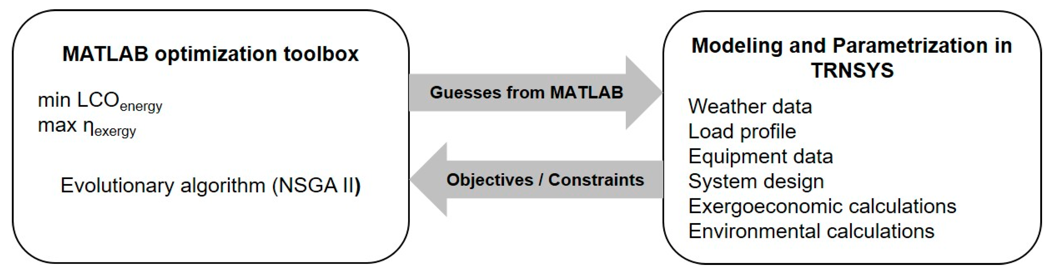
5.1. Multi-Objective Optimization

The mentioned objective functions and constraints (Section 4.3) are specified in MATLAB. Initial guesses from MATLAB are written into a text file, which is read by TRNSYS. The corresponding values of the objective functions and constrains are calculated in TRNSYS and written into another text file, which is read by MATLAB. The coupling happens once at the beginning and once at the end of each simulation. The algorithm initially tries to find the points, which do not violate the constraints, and assesses the objectives afterwards. This procedure is repeated for each scenario until the best Pareto front, which is the loci of the most optimal solutions, is selected. Figure 6 illustrates the computational model.

5.2. System Simulation

The calculated load profile, as shown Figure 1, is given as a time series to TRNSYS simulation studio. Type 557, which is based on a duct storage model [53], is used for BTES modeling. It can be used to simulate thermally interacting BHEs within a cylindrical storage volume. The validity of Type 557 has already been proven in many practical projects (e.g., [54]). Design parameters (

Table 5. Main TRNSYS parameters.

Component	Parameter	Value	Component	Parameter	Value
BTES	BHE type	2U	HP	1st stage cooling capacity	102.9 kW
Type 557	Boreholes in series	6	Type 1221 c	2nd stage cooling capacity	56.1 kW
	Borehole radius	0.065 m		1st stage cooling power	22.9 kW
	Pipe outer/inner radius	0.016/0.0131 m		2nd stage cooling power	10.2 kW
	Pipe thermal conductivity	0.38 W/m.K		1st stage heating capacity	86.9 kW
	BTES thermal conductivity	2.6 W/m.K		2nd stage heating capacity	49.8 kW
	BTES heat capacity	2080 kJ/m3.K		1st stage heating power	28.9 kW
	Grout thermal conductivity	2 W/m.K		2nd stage heating power	15.1 kW
	Fluid specific heat (EG 25%)	3.811 kJ/kg.K
BST	Number of tank nodes	30	HP	Cooling capacity	59.8 kW
Type 534	Number of ports	4	Type 927 c	Cooling power	13 kW
	Aspect ratio	2.5		Heating capacity	50.6 kW
	Loss Coefficient	0.15 W/m2.K		Heating power	18 kW
Pump	Total pump efficiency	60%	Boiler	Efficiency	95%
Type 110			Type 700
Thermostat	Dead band temperature	0.5 K	HEX	Effectiveness	0.895
106, 113			Type 91

^c Values at rated conditions of the catalog and differ from normalization values.

) are based on standard libraries [49] and location-specific parameters are chosen according to experimental data [55]. The BST is modelled with type 534, which divides the tank’s volume into different stratified layers and solves the energy balance equation to calculate a time-dependent temperature change of the fluid inside the tank at different levels. It has also been used for the simulation and validation of similar studies [56,57,58]. The loss coefficient (Table 5) is based on the data from a manufacturer [59] and matches practical investigations [54,56]. Types 927 and 1221 are used for simulating single- and double-stage HPs, respectively. According to inlet source- and load-side temperatures and flow rates, output capacity and power consumption of HPs are calculated based on the provided catalog files. The catalogs are chosen so that they can be representative of the operation of common HPs on the market [32,60]. The chosen catalogs are transformed into external files with normalized values, which are read by the HP types and a parametric study was conducted to check the compatibility of the provided files and the original manufacturers’ catalogs. Type 700 was used to model the GBs, which are assumed to be condensing gas boilers with a high energetic efficiency of around 95% [34]. Important parameters of the other components including heat exchangers, pumps and thermostats were mainly selected based on manufacturer [30] or experimental [54] data and are illustrated in Table 5.

6. Results

Figure 7 displays the area assessed by the optimization algorithm, including points that violate the constraints. As it is expected, the algorithm initially tries to find a minimum, where increasing the efficiency decreases the cost. From that point on, a further increase in efficiency results in higher costs and the algorithm searches for the loci of the points with maximum efficiencies and minimum costs.

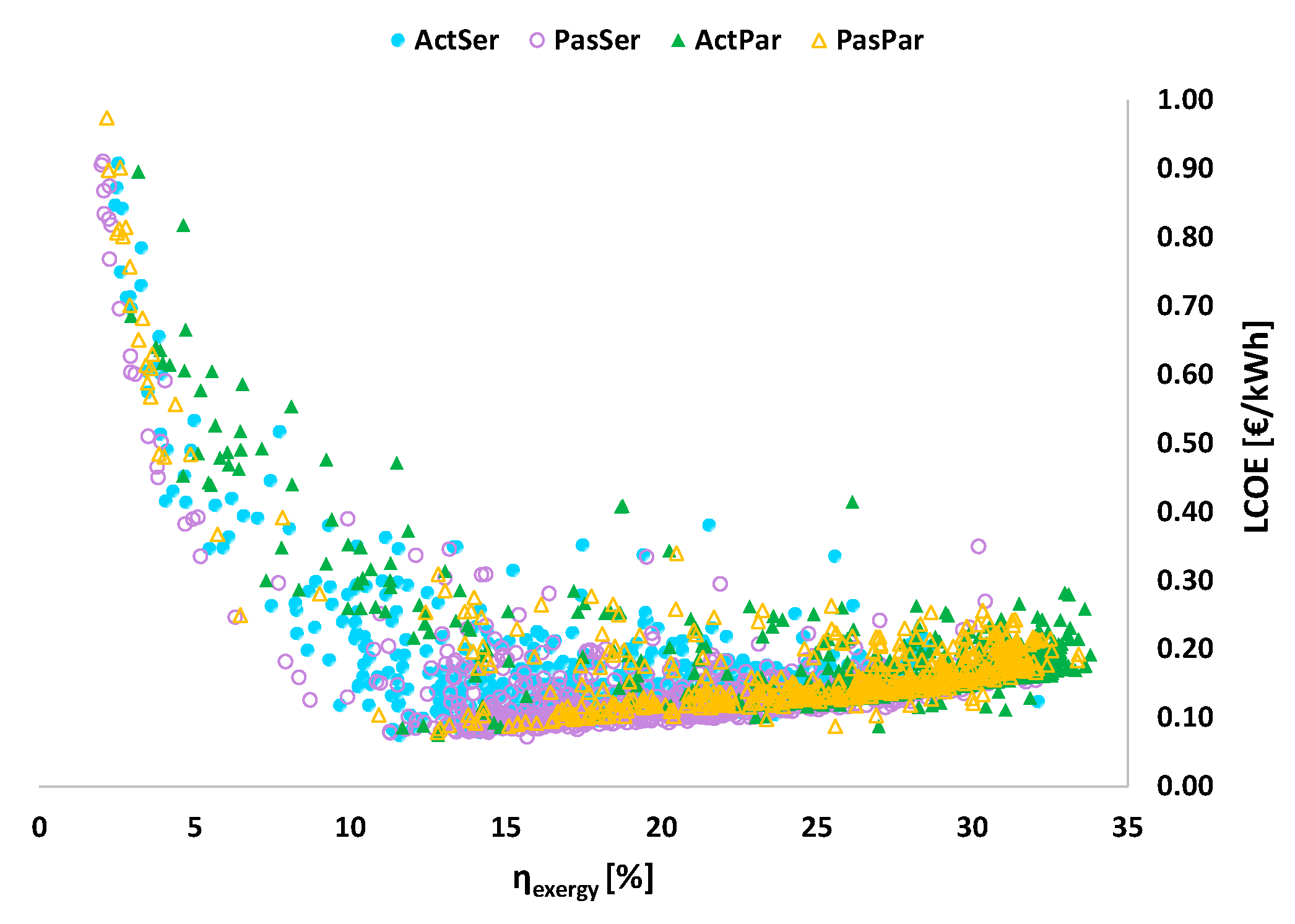
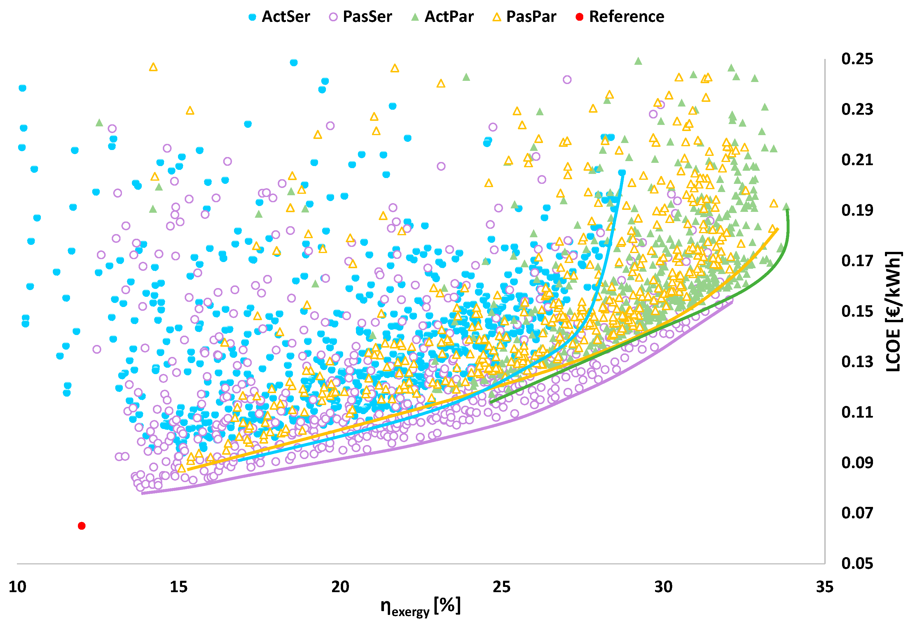
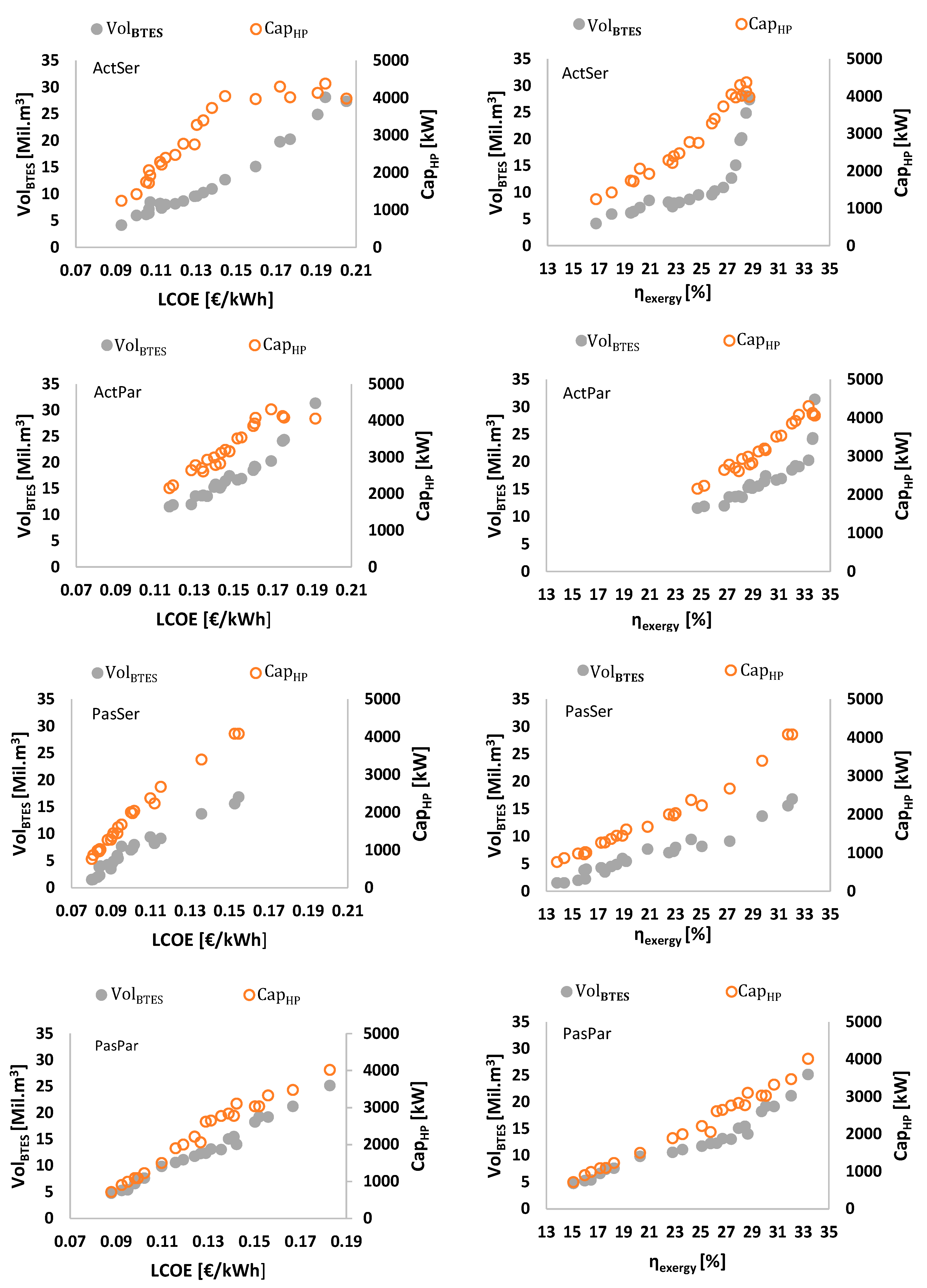
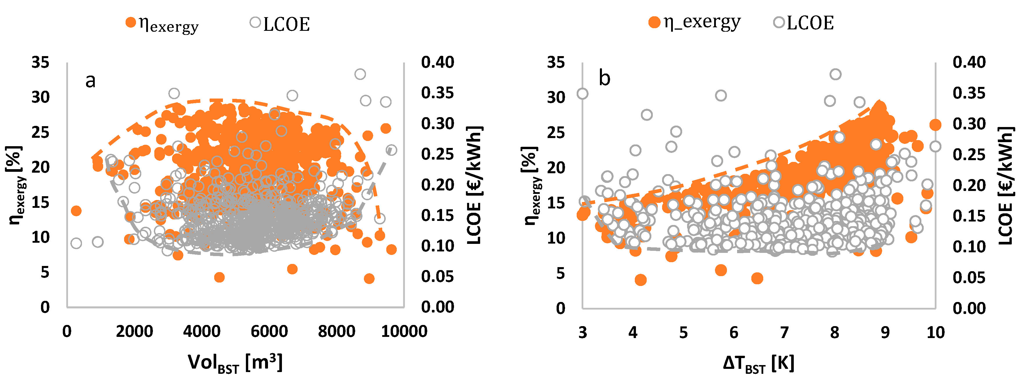
6.1. Pareto Efficient Solutions

Figure 8 shows the local evaluations by the algorithm for finding the points which do not violate the constraints. The non-dominated points for each scenario are located on a Pareto front, which is closest to the bottom right corner (Figure 8 and Figure 9). On the Pareto fronts $\mathrm{LCOE}$ ranges from aimately 8 to 20 ct/kWh and ${\mathsf{\eta }}_{\mathrm{exergy}}$ from 14 to 35%. For the reference scenario those numbers are 6.5 ct/kWh and 12%, respectively.

When HPs are designed to cover the whole $\Delta {\mathrm{T}}_{\mathrm{BST}}$ i.e., in the serial scenarios, supplying cooling load passively (PasSer) leads to more economical and more efficient designs. This means designs with equal efficiency have lower costs and designs with equal costs are more efficient for the PasSer scenario than for the ActSer scenario. Especially, when it comes to efficiencies higher than approx. 27%, costs for the ActSer scenario show a much steeper increase than the other scenarios.

In contrast, when double stage HPs are connected serially and cover almost half of $\Delta {\mathrm{T}}_{\mathrm{BST}}$ i.e., in the parallel scenarios, active cooling (ActPar) is superior to passive cooling (PasPar) for designs with efficiencies higher than approx. 25%. However, for less efficient designs, passive cooling becomes more economical again than active cooling.

When comparing the serial with the parallel connection of HP and GB in heating operation, it is obvious that the parallel scenarios generally are able to reach higher efficiencies than their parallel counterparts with equal cooling mode, while the serial systems are generally advantageous when lower efficiencies are in demand as they reach lower costs.

However, the serial scenario with passive cooling (PasSer) also reaches exergetic efficiencies up to 32% and thus shows the most economical designs for a wide efficiency range, except for the highly efficient design points with exergetic efficiencies over 32%. Here, ActPar scenario becomes beneficial, as it reaches efficiencies up to almost 34%.

The ranges of the selected optimized variables for each scenario are given in

Table 6. Ranges of the optimized solutions on the Pareto fronts.

Scenario	LBHE [m]	NBHE	SBHE [m]	CapHP [kW]	VolBST [m3]	ΔTBST [K]
ActSer	95–155	294–1194	10.7–15.1	1264–4400	917–6847	7.9–9.1
ActPar	156–200	426–924	11.4–15	2175–4349	1260–5630	-
PasSer	143–169	222–1026	7.3–11.6	809–4097	795–6356	6.7–9.8
PasPar	159–224	174–1008	11.3–14	759–4046	1459–7045	-

. Scattering plots showing the distribution of the volume of BTES (${\mathrm{Vol}}_{\mathrm{BTES}}$) and ${\mathrm{Cap}}_{\mathrm{HP}}$ on the pareto front of each scenario and their effect on the objective functions are illustrated in Figure 10. ${\mathrm{Vol}}_{\mathrm{BTES}}$ (Equation (10) [53]) is selected because it gives a relation for three of the main optimization variables including ${\mathrm{N}}_{\mathrm{BHE}}$, ${\mathrm{L}}_{\mathrm{BHE}}$ and ${\mathrm{S}}_{\mathrm{BHE}}$. Consequently, by choosing the mentioned variables from the optimized ranges in Table 6, an optimum design point with a corresponding HP capacity can be selected using Figure 10. Although there are exceptions, it can be generally implied that the increase in ${\mathrm{Vol}}_{\mathrm{BTES}}$ as well as ${\mathrm{Cap}}_{\mathrm{HP}}$ results in more efficient, but more expensive, design points. Figure 11a shows ${\mathrm{Vol}}_{\mathrm{BTES}}$ for the local search of the ActSer scenario and its effect on the objective functions. ${\mathsf{\eta }}_{\mathrm{exergy}}$ and $\mathrm{LCOE}$ have their optimum values in the middle ranges of the chosen boundaries. Moreover, a higher $\Delta {\mathrm{T}}_{\mathrm{BST}}$ (Figure 11b) mainly results in a more efficient and more economical design, with ${\mathsf{\eta }}_{\mathrm{exergy}}$ showing a higher sensitivity. The objective functions of the other serial scenario, PasSer, have approx. the same sensitivity to ${\mathrm{Vol}}_{\mathrm{BTES}}$ and $\Delta {\mathrm{T}}_{\mathrm{BST}}$.

$${\mathrm{Vol}}_{\mathrm{BTES}}=\mathsf{\pi }\times {\mathrm{N}}_{\mathrm{BHE}}\times {\mathrm{L}}_{\mathrm{BHE}}\times {\left(0.525\times {\mathrm{S}}_{\mathrm{BHE}}\right)}^2$$

(10)

For further analysis of the scenarios, three characteristic Pareto efficient designs (further referred to as Characteristic Designs) are chosen for each scenario. These include the most economical, the most efficient and a compromise solution, which is the closest to the corner (Figure 8 and Figure 9).

Table 7. The economic, the compromise and the efficient system designs of each scenario.

Scenario		LCOE [ct/kWh]	ηexergy [%]	LBHE [m]	NBHE	SBHE [m]	CapHP [kW]	VolBST [m3]	ΔTBST [K]
ActSer	Economical	9.27	16.77	112	294	12.0	1264	2989	7.95
	Compromise	12.37	24.05	116	702	11.0	2782	4646	8.59
	Most efficient	19.45	28.49	136	1036	15.1	4400	3281	8.91
ActPar	Economical	11.73	24.69	190	426	12.8	2175	1260	-
	Compromise	14.37	29.42	170	660	12.6	3136	5420	-
	Most efficient	19.16	33.80	175	918	15.0	4097	4307	-
PasSer	Economical	8.02	13.81	145	222	7.4	809	3556	6.68
	Compromise	10.00	22.47	143	480	10.9	2007	3008	9.50
	Most efficient	15.47	32.04	153	942	11.6	4097	4658	9.65
PasPar	Economical	8.79	15.10	185	174	12.9	758	4186	-
	Compromise	12.66	25.78	164	636	11.6	2073	4007	-
	Most efficient	18.29	33.38	162	1008	13.3	4046	5128	-

lists their most important design parameters as well as the corresponding ${\mathsf{\eta }}_{\mathrm{exergy}}$ and $\mathrm{LCOE}$. Bold lines show the most economical and the most efficient layouts overall, which belong to PasSer and ActPar scenarios. The economical, the compromise and the most efficient layouts of each scenario are referred to with ECO, COMP and EFF respectively.

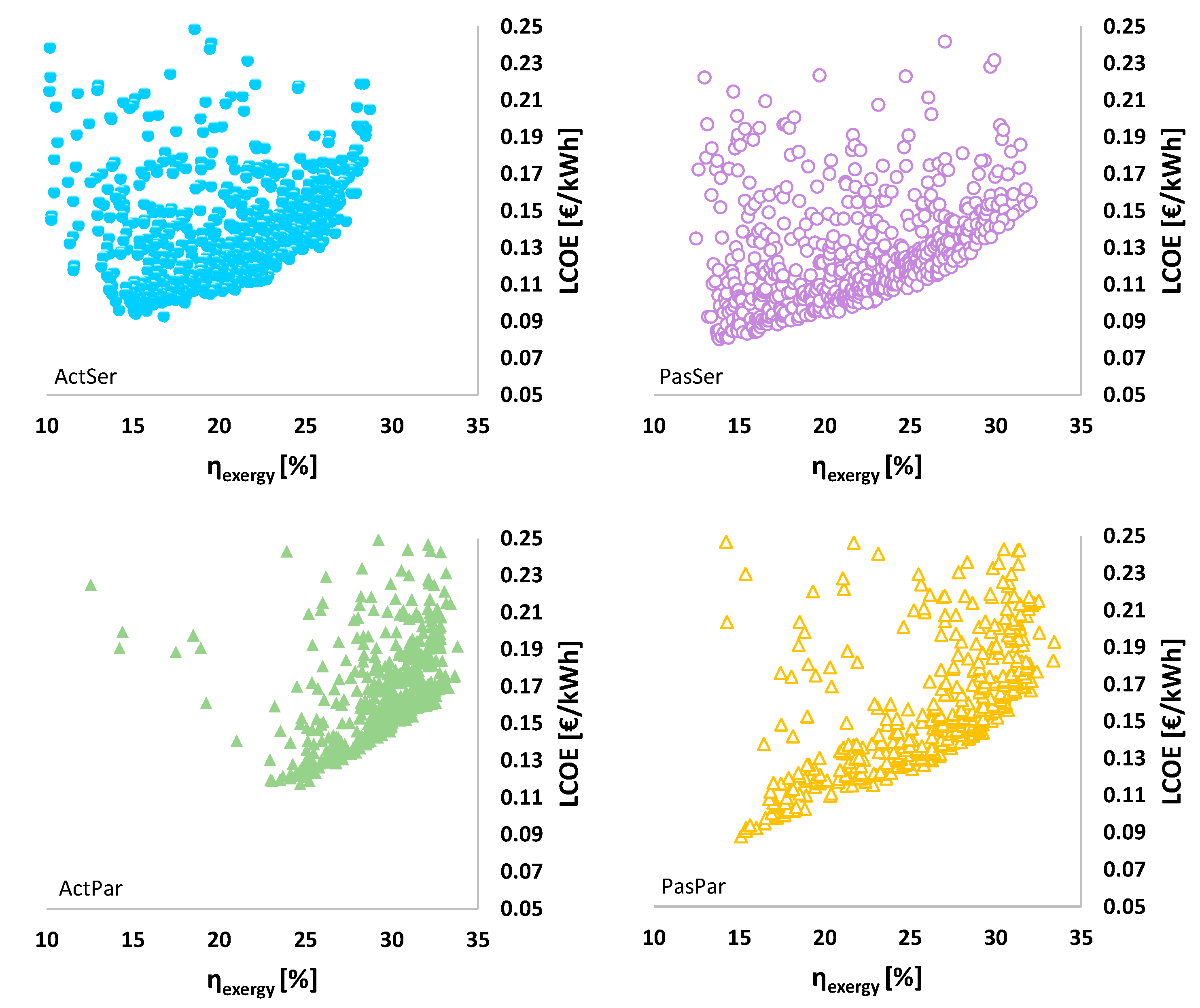
6.2. Scenario Analysis

To gain deeper insight into the coherencies of the results and the differences for the four scenarios, the component-wise exergy destruction and loss (Figure 12) and composition of $LCOE$ (Figure 13, Figure 14, Figure 15 and Figure 16) for all 12 Characteristic Designs (cf. Section 6.1.) as well as for the reference case are presented and discussed in the following sections.

6.2.1. Reference Case

As mentioned earlier, for the reference scenario the total heating demand is supposed to be supplied by condensing GBs and the cooling demand by air-source HPs. Therefore, it has one design point and not a pareto front. Despite high energetic efficiency, condensing GBs have a very low exergetic efficiency as natural gas with its high exergy content is converted to generate low exergy heat [18]. The calculated ${\mathsf{\eta }}_{\mathrm{exergy}}$ of the condensing GBs and the air-source HPs are 11% and 21%, respectively. Consequently, the calculated overall average ${\mathsf{\eta }}_{\mathrm{exergy}}$ is 12% and its corresponding exergy destruction is 240 GWh/30yrs. Moreover, using the cost functions in Table 2 and Table 3, the $\mathrm{LCOE}$ of the reference scenario is 6.5 ct/kWh. The largest exergy destruction belongs to the most economical design from PasSer scenario and is 197 GWh/30yrs (Figure 12), which is almost 22% lower than the reference case. However, its $\mathrm{LCOE}$ is 23.5% higher.

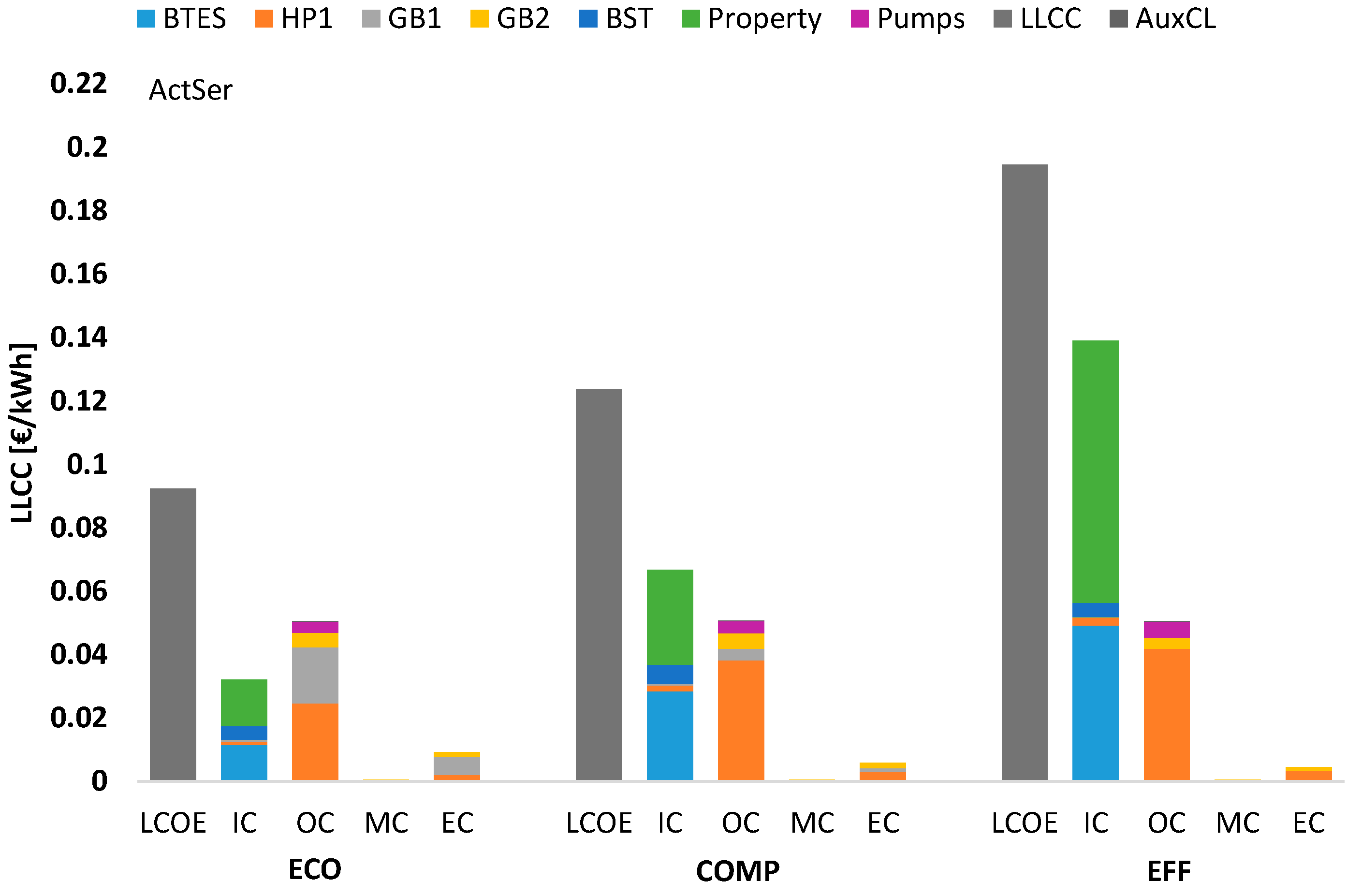
6.2.2. ActSer–Active Cooling and Serial Heating

The total exergy destruction is reduced significantly by moving from the economical to the most efficient point (Figure 12). For the economical design, the highest exergy destruction is from the GBs followed by the HP. For the compromise solution, these are almost balanced and for the most efficient design, the HP dominates exergy destruction. Exergy destruction of the BST and the BTES show the lowest number compared to the other system components.

Figure 13 shows the $\mathrm{LCOE}$ of the Characteristic Designs for the ActSer scenario. For the economical design ICs are lower than OCs. This relation is reversed for the most efficient and compromise designs. It is almost three times higher for the most efficient design. GBs have the lowest share in ICs, even for the economical layout. The largest share is either from the BTES or from the property, which is used for installing the BTES. Combined, they make up more than 94% of the ICs of the most efficient layout. The OCs remain almost the same for all designs, with HPs being the major part for the compromise and the most efficient designs. The power consumption of the pumps is mainly required to circulate the fluid inside the BTES and increases with its size. However, it also depends on ${\mathrm{N}}_{\mathrm{BHE}}$, which specifies the design pressure drop that the pump is required to meet. MCs are very low in comparison to the other costs and increase slightly from the economical to the most efficient design point. This is mainly due to the increased HP capacity. The highest ECs can be observed for the economical design and originates from the high share of the GB.

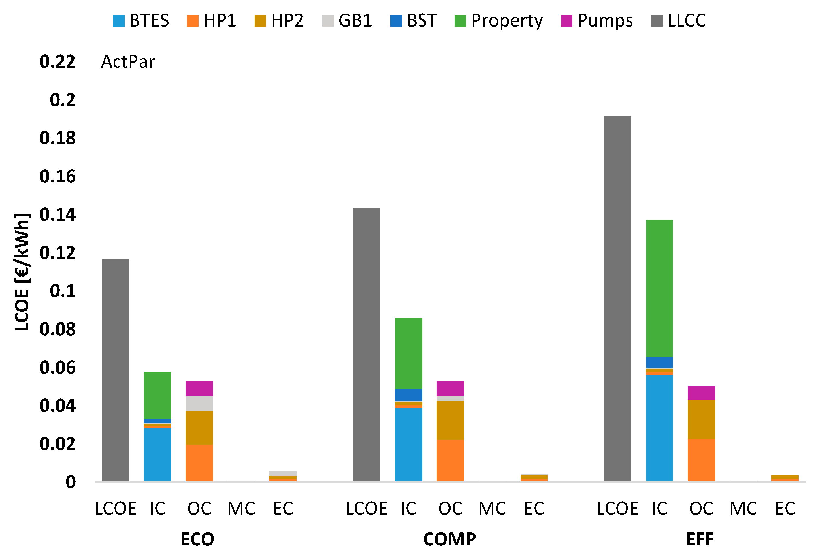
6.2.3. ActPar–Active Cooling and Parallel Heating

ActPar scenario comprises the most efficient layout among all the layouts (Figure 8, Table 7). Like for the other scenarios, the most efficient layout has the lowest share of GBs for covering the peak demand and the highest share of HPs in heating load supply. In heating mode, entering temperatures on the BTES side of HP1 are higher than HP2 with lower load side temperatures. In cooling mode, HP1 has lower BTES side and load side temperatures. As HP2 has lower exergy destruction in heating and cooling modes, it can be concluded that the load side temperature has more effect on the exergetic performance of the HPs in the proposed system layout (Figure 12). Increased flow rates are required to maintain the same design temperature difference on both sides of the HPs in comparison to the other scenarios. This results in higher power consumption of the circulating pumps and the associated exergy destruction. Like previous scenarios, the exergy destruction of the BST and the BTES are the lowest in comparison to the other components.

As shown in Figure 14, ICs are higher than OCs for all three Characteristic Designs. The BTES and the property have the highest shares in ICs, followed by the BST. HPs contribute to a high percentage of OCs, which increases from the economical to the most efficient one because of larger HP capacities. The higher power consumption of the circulating pumps also results in their higher share in OCs, which increases for higher efficiencies. Like previous scenarios, MCs increase and ECs decrease from the economical to the most efficient design.

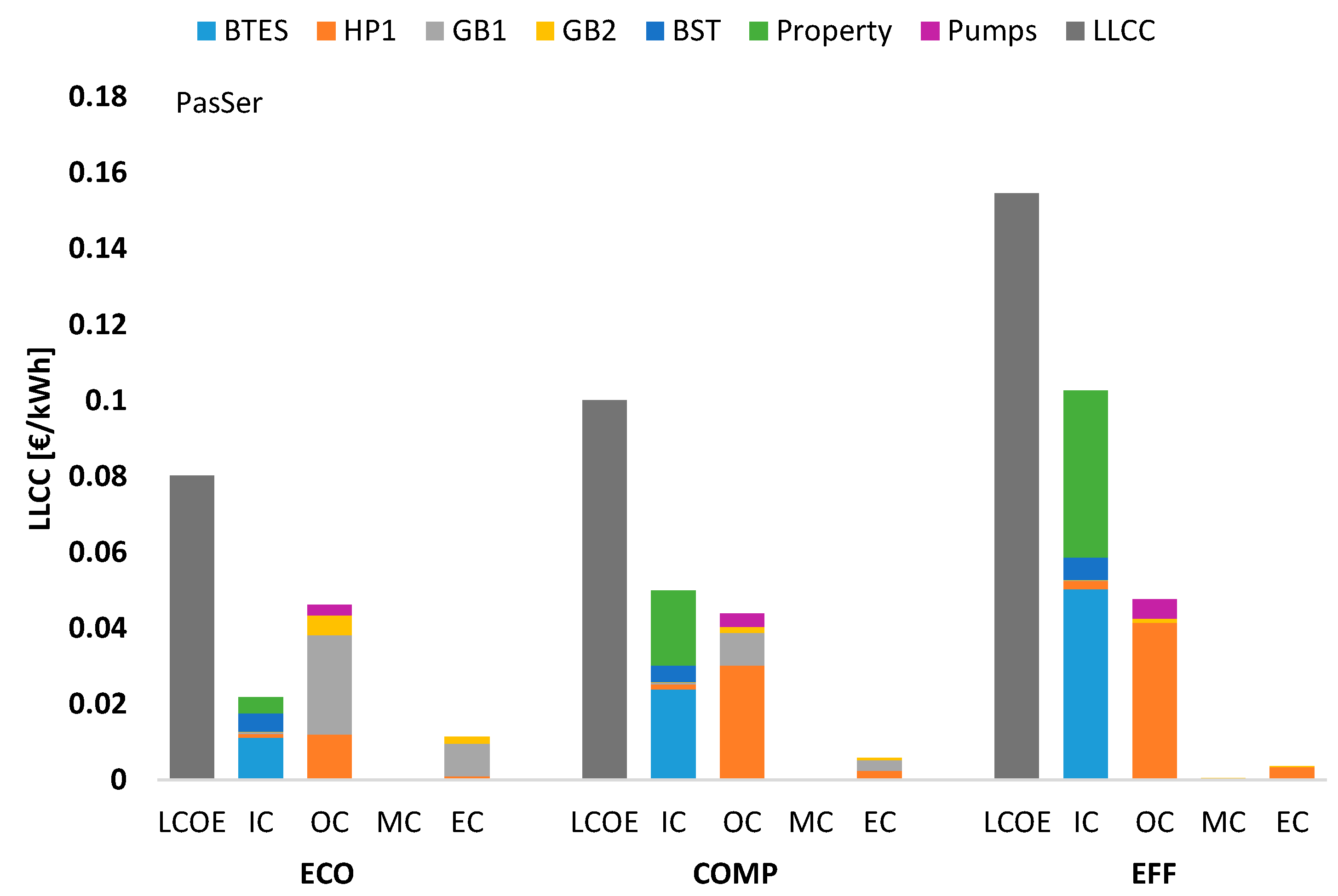
6.2.4. PasSer–Passive Cooling and Serial Heating

PasSer scenario shows the most economical and least efficient design point of all Characteristic Designs (Table 7). As shown in Figure 12, the highest exergy destruction results from the GBs followed by the HP. Here, due to the passive cooling strategy, the exergy destruction of the HP in cooling mode is omitted and that of the HEX is added, which is the lowest among other components. Overall, HEX, BST and BTES show the lowest share in exergy destruction.

As for the ActSer scenario, OCs remain almost the same for the three design options. ICs are lower than OCs for the economical layout and more than double for the most efficient one. The largest share of ICs is either from the BTES or from the land use, except for the economical design, for which the property costs are much lower than the ICs of the BTES due to the lowest spacing. Like for the ActSer scenario, MCs are negligible and increase with efficiency. The highest ECs can be observed for the economical point and decrease for more efficient systems.

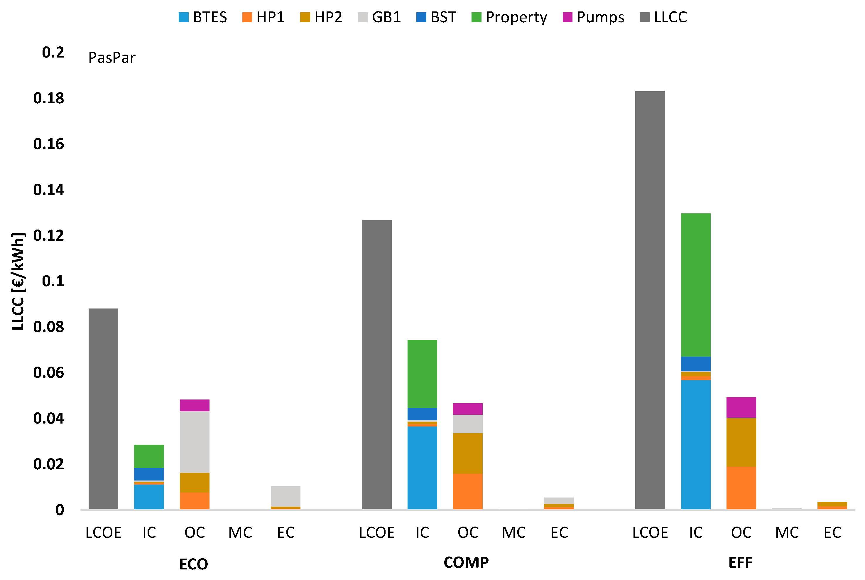
6.2.5. PasPar–Passive Cooling and Parallel Heating

As for all scenarios, the most economical layout has the highest exergy destruction, which decreases from the economical to the most efficient solution (Figure 12). The exergy destruction of the HP in cooling mode is replaced with that of the HEX and increases for larger BTES volumes due to higher flow rates. In accordance with the ActPar scenario, the overall exergy destruction of HP1 is higher than HP2, which implies the importance of load side temperature. The relatively high flow rates of the pumps result in a high share of the overall exergy destruction, which increases from the economical to the most efficient design.

Total and component-wise $\mathrm{LCOE}$ of the PasPar scenario are illustrated in Figure 16. The economical layout has a high share of GB in heating load supply. Therefore, the OCs and ECs as a result of gas consumption are approx. 55% and 12% of the $\mathrm{LCOE}$, respectively. The most efficient solution has the largest number of BHEs and the largest spacing of all Characteristic Designs. Consequently, the ICs are the dominating part of the $\mathrm{LCOE}$ with a share of above 65%, which is again caused by high costs of the BTES and the associated property. MCs are a minor share and increase from the economical to the most efficient design. ECs make up almost 12% of the $\mathrm{LCOE}$ of the economical layout and decrease with increasing efficiency.

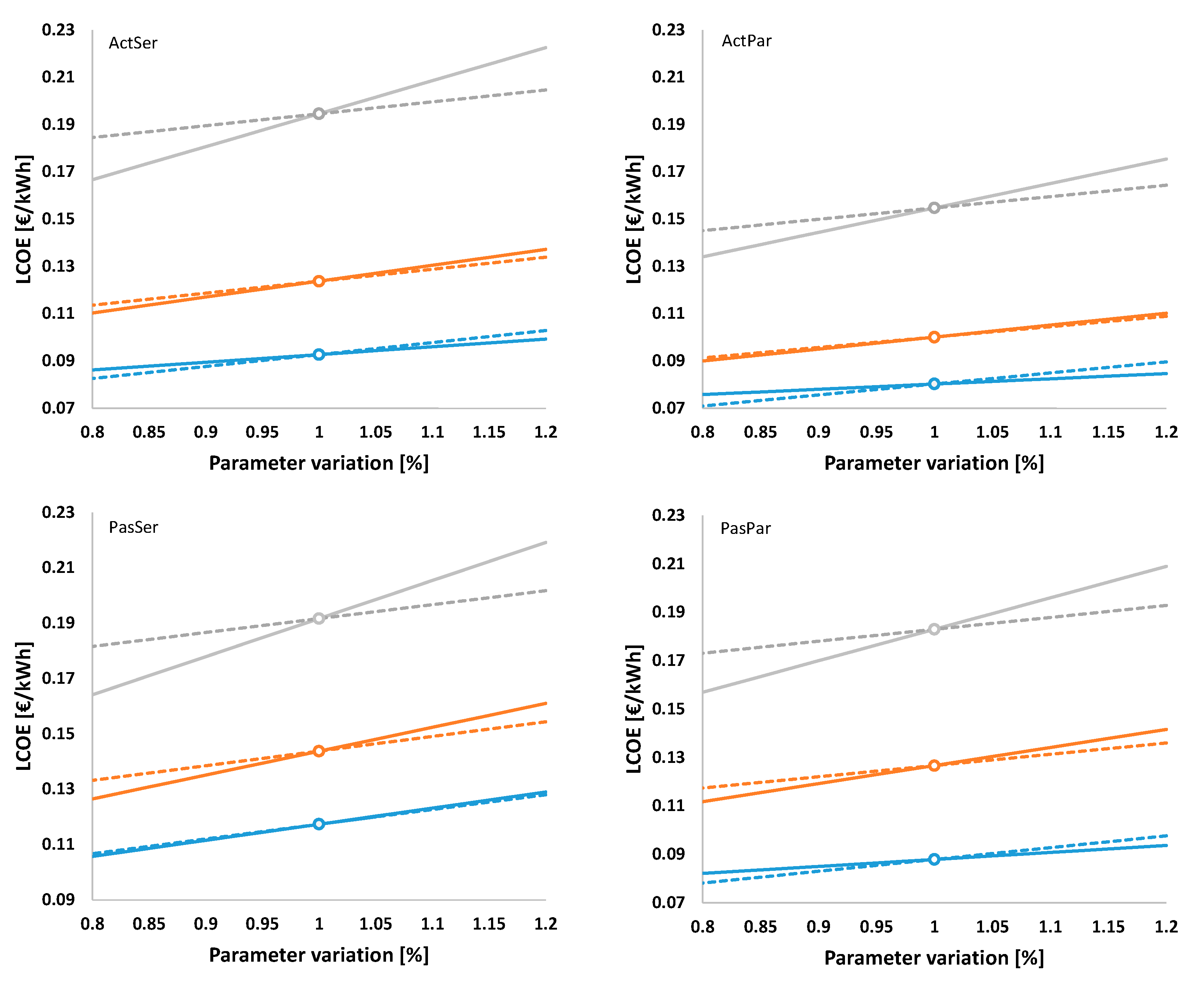
6.3. Sensitivity Analysis

6.3.1. Variation of Initial Costs and Energy Costs

In a one-at-a-time sensitivity analysis, effects of 20% variation in ICs and OCs on the $\mathrm{LCOE}$ of the Characteristic Designs (cf. Section 6.1.) are assessed (Figure 17). Changing the ICs has a stronger effect than changing OCs for the most efficient designs (gray lines). In contrast to that, the OCs show a higher impact on the $\mathrm{LCOE}$ for the economical layouts. By reducing OCs and ICs of the economical point of PasSer scenario by 20%, its $\mathrm{LCOE}$ decreases to 7.0 ct/kWh and 7.6 ct/kWh, respectively. Moreover, the influence of varying OCs on $\mathrm{LCOE}$ of different scenarios is almost the same for all of the chosen points of each scenario. This is different from varying ICs, which has a higher influence on more efficient layouts with larger BTES volumes and smaller GB capacities.

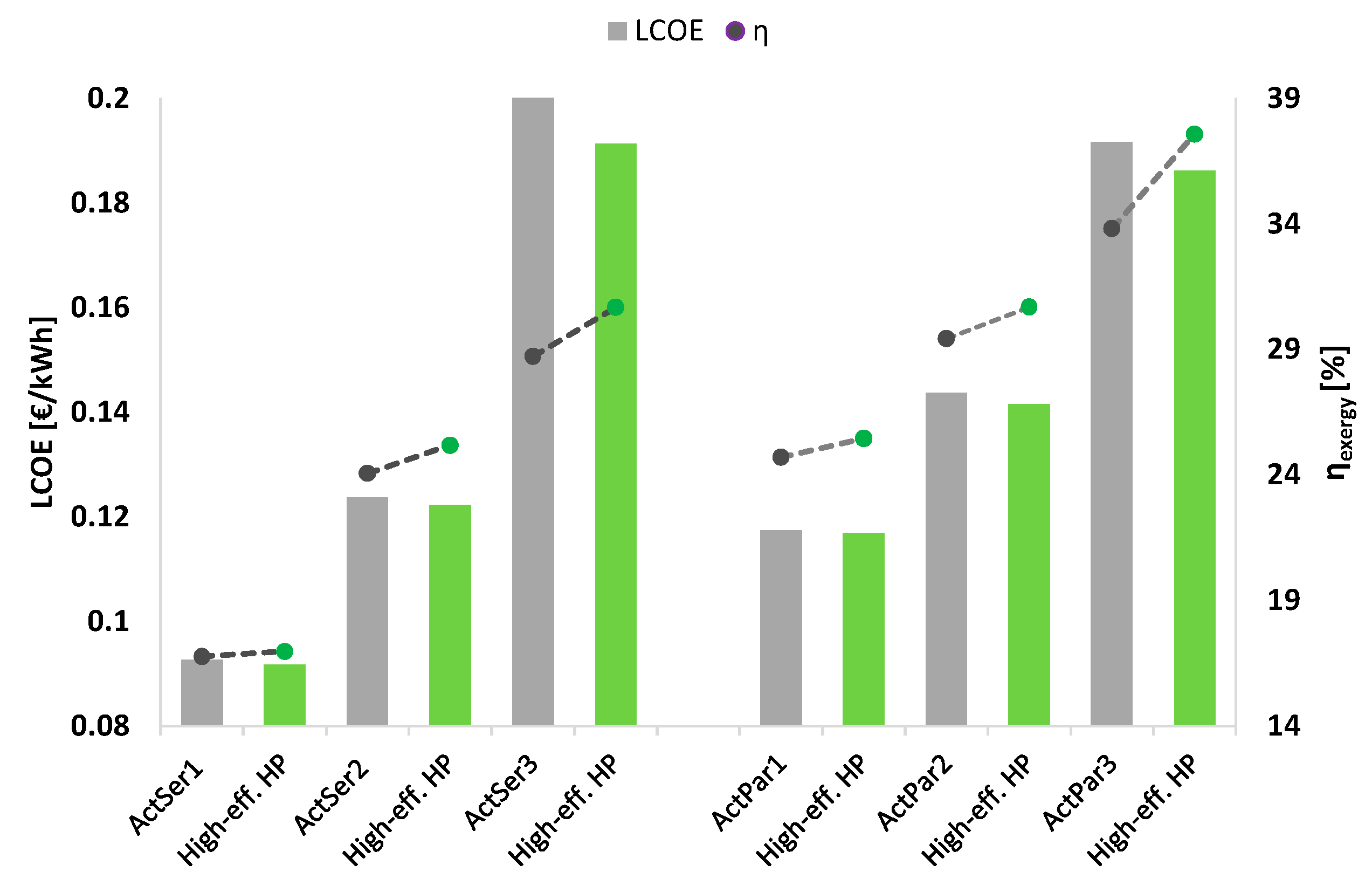
6.3.2. Changing Heat Pump Type

As mentioned earlier, HPs contribute to a high percentage of exergy destruction and $\mathrm{LCOE}$. In the previous parts of the study, a commonly used standard heat pump type was considered. However, to capture the effects of increasing HP efficiencies, the HPs of the active scenarios are replaced by a more efficient HP type [61] with a 20% higher nominal COP (Figure 18). As expected, total exergetic efficiency increases and $\mathrm{LCOE}$ decreases by using a more efficient HP. This is more pronounced for the most efficient scenarios because of their higher contribution of HPs. For the most efficient point of ActPar scenario, the overall exergetic efficiency increases by 11.2% and the cost decreases by 2.9%. Therefore, using HPs with higher COPs has a larger effect on the exergetic efficiency than on the cost.

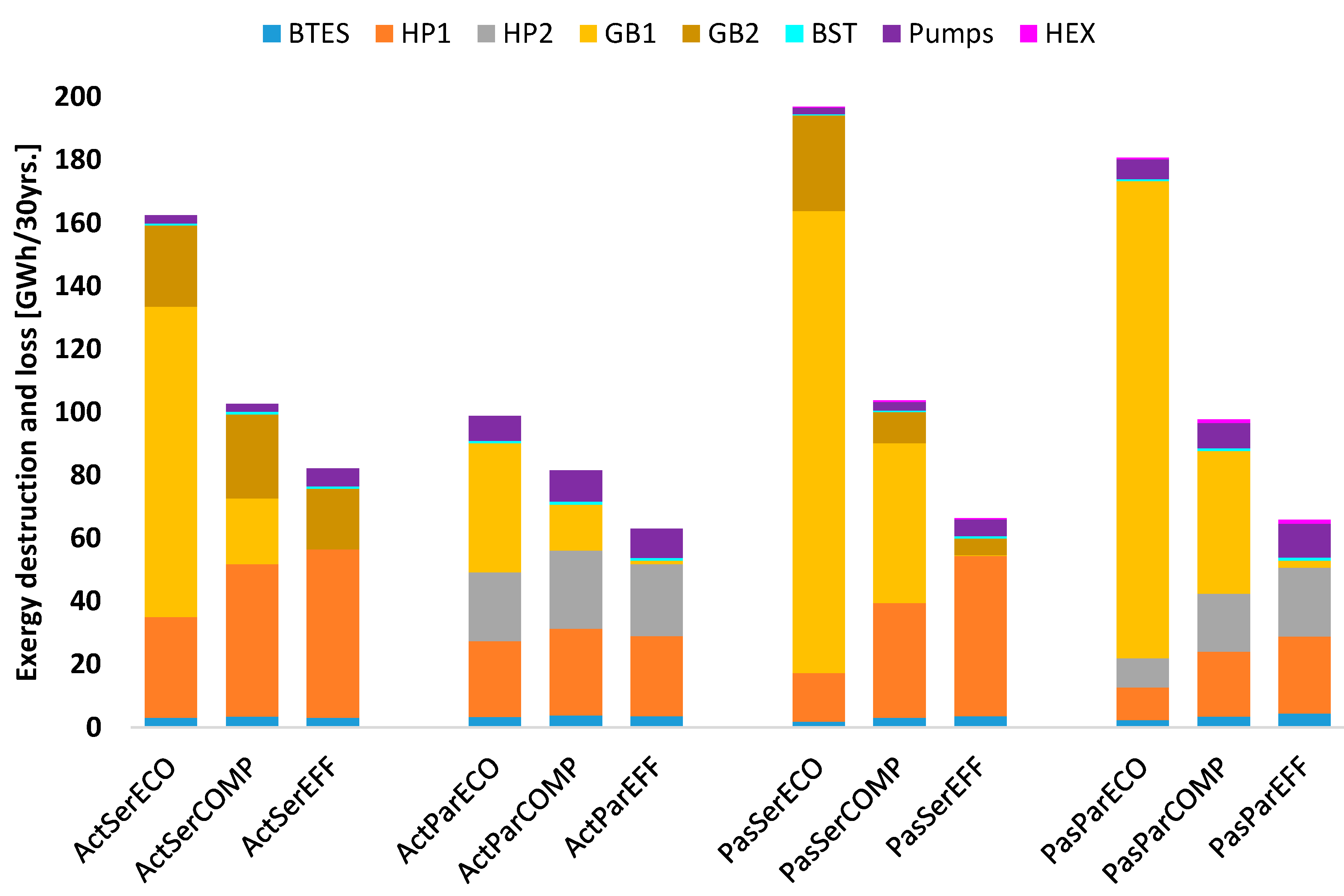
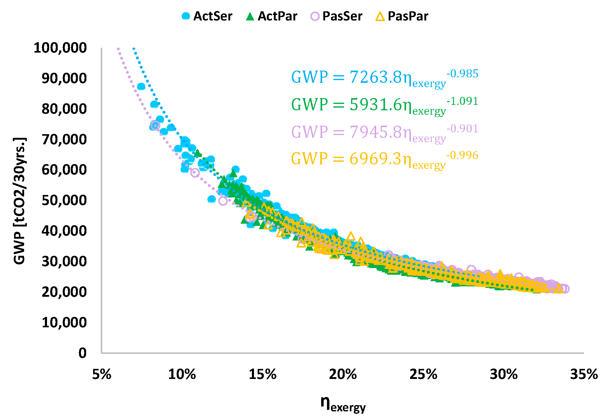
6.4. Exergy and Global Warming Potential

Reducing environmental impacts plays a major role in global transition to renewable energies. As mentioned earlier, the LCA method lacks thermodynamic assessment. Moreover, increasing exergy efficiency reduces environmental impacts [19]. To have a rough estimation of how they are related to each other, GWPs of the evaluated system layouts were calculated parallel to the optimization procedure in each simulation run. To assess GWPs, the GWPs associated with electricity and gas consumption are calculated based on the functions in Table 3. The GWP as a result of the production of each system component (${\mathrm{GWP}}_{\mathrm{prod,n}}$) is calculated using available online data [20,62]. Finally, Equation (11) was used for the calculation of each component’s GWP and then summed up for the overall GWP of each system layout.

$$\mathrm{GWP}={{\displaystyle \sum }}_{\mathrm{n}=0}^{{\mathrm{n}}_{\mathrm{end}}}{\mathrm{GWP}}_{\mathrm{elec},\mathrm{n}}+{\mathrm{GWP}}_{\mathrm{gas},\mathrm{n}}+{\mathrm{GWP}}_{\mathrm{prod},\mathrm{n}}$$

(11)

Results of calculating GWP for different design points of the scenarios and their corresponding exergetic efficiency are illustrated in Figure 19. As expected, an increase in exergetic efficiency leads to a decrease in environmental impacts. This trend can be expressed by a function. Therefore, the exergoeconomic optimization results in system layouts with lower GWP by taking thermodynamic inefficiencies into consideration.

7. Discussion

7.1. Limitations

On the one hand, a generic study of a complex system requires many simplifications and assumptions, which has its own drawbacks and may cause uncertainties. On the other hand, implementing too much detail is computationally expensive and may lead to unexpected results, which can prevent the definition of generic rules and guidelines. A proper approach can be conducting a generic study which is followed by detailed assessments, when it comes to practical applications. The following simplifications and assumptions were considered in this study:

• Load scenarios were calculated based on German standards for renovated buildings. Results of this study can provide design guidelines for buildings with different performances as long as they have the same temperature ranges and similar functionalities. The definition of the DHC grid temperature levels were based on the target return temperatures of low-temperature grids. However, due to simplification, the DHC grid configuration and the associated costs and exergy destruction rates are not considered in this study. Future studies, which assess different building types and grid configurations, and consider DHC pipes and circulation pumps as main components of BTES-assisted DHC grids are required for more comprehensive analysis.
• To set up an optimization algorithm according to real HP data within a wide range, it is assumed that the selected HP consists of a number of HP modules with similar performances. However, there is a maximum limit for the number of HP modules to avoid technical issues in practice. Moreover, according to an inquiry from a HP manufacturer, large-scale HPs can be ordered with desired technical specifications which are easily compatible with part-load applications.
• It is assumed that GBs cover the load which cannot be supplied by the ground loop, without considering the effect of part-load ratio on its performance. However, modulating GBs mainly have a minimum turn-down ratio, which specifies the minimum acceptable part-load ratio. For a more detailed assessment the boiler and the combustion efficiencies need to be provided as a function of entering liquid temperature and device part-load ratio.
• The selected BST volume by the optimization algorithm is allocated to one tank with an aspect ratio (the ratio of height to diameter) of 2.5, according to an estimation regarding an efficient design as well as the maximum acceptable tank height for large-scale applications. Splitting the selected volume into multiple tank units with different aspect ratios can be considered as a future study.
• The project lifetime is considered to be 30 years. Approx. 2000 evaluations, each taking around 20 min, were required for the initial convergence of the optimization algorithm. Consequently, a time step of one hour was considered for the simulations. However, a more detailed assessment required shorter time steps down to a few minutes, which also enables an application of more exact control strategies. The optimization always results in better solutions with shorter time steps and a larger number of evaluations.
• The heat transfer mechanism of the BTES is considered to be conductive. It is also assumed that BTES is installed in the ground with a uniform thermal conductivity and heat capacity. However, in real geothermal applications convective heat transfer might exist and ground thermal characteristics might not be uniform. Moreover, there are always regional limitations for the implementation of large-scale geothermal projects, e.g., unfavorable subsurface conditions or restrictions due to groundwater protection.
• The IC functions (Table 2) are based on the available literature, which are mainly defined by having data from real projects in a specific range. However, due to the large ranges of the optimization boundaries, it is assumed that extrapolation is acceptable. Regarding OCs (Table 3), energy cost functions are specified by the predicted costs from the economic studies for the years 2030 and 2050 and assuming a linear interpolation between the available data points. Similar assumptions have been made for the environmental emissions and the associated costs. Consequently, cost functions are subject to large uncertainties and the sensitivity analysis was done with the purpose of lowering these uncertainties.

7.2. Discussion of Results

The PasSer scenario shows the most economical designs for a wide efficiency range of up to 32%. This can be explained by the passive cooling strategy, which leads to an omission of HPs that are usually responsible for significant amounts of exergy destruction and high OCs. Moreover, lower pumping power, due to covering the whole heating temperature shift in serial scenarios, overcompensates higher COPs in parallel scenarios because of lower temperature shifts by HPs.

For the highly efficient designs with exergetic efficiencies over 32%, ActPar scenarios show the best results. Large values for both ${\mathrm{Cap}}_{\mathrm{HP}}$ and ${\mathrm{Vol}}_{\mathrm{BTES}}$ are needed to reach such high exergetic efficiencies. Consequently, higher COPs of HPs in parallel scenarios have a larger impact and overcompensate lower power consumption of circulation pumps in serial scenarios. However, in cooling mode, a higher power consumption of the pumps due to the lower temperature shift on BTES side has a slightly higher share in inefficiencies and losses.

For the serial scenarios (Figure 11), higher $\Delta {\mathrm{T}}_{\mathrm{BST}}$ mainly results in a more efficient and more economical design, with ${\mathsf{\eta }}_{\mathrm{exergy}}$ showing a higher sensitivity. This indicates that the improved performance of the BST, due to better stratification and less mixing losses, overcompensates the lower COPs of the HPs due to higher temperature shifts. Therefore, the algorithm favors scenarios with higher values for $\Delta {\mathrm{T}}_{\mathrm{BST}}$.

The optimization of the serial layouts leads to the maximum possible temperature shift of the grid by the HPs, which makes them similar to the HPs in parallel scenarios. However, due to weaker performance of HPs for covering high temperature shifts, ${\mathsf{\eta }}_{\mathrm{exergy}}$ does not exceed 28.5% with a $\mathrm{LCOE}$ of 19.45 ct/kWh for ActSer scenario. This corresponds to a layout in which GB1 is omitted and the supplementary load is supplied by GB2 serially. A Pareto efficient design point of the ActPar scenario with the same ${\mathsf{\eta }}_{\mathrm{exergy}}$ has an $\mathrm{LCOE}$ of 13.86 ct/kWh. Therefore, to move towards more economical points in the serial scenarios, both GBs are required, and a splitter sends the fluid to either the HPs and GB2 or to the GB1. The GB1 has a share between 0 and 49% of the total heating demand on the Pareto front of the ActSer scenario. Similarly, for the PasSer scenario, the point with the highest ${\mathsf{\eta }}_{\mathrm{exergy}}$ of 32% has $\mathrm{LCOE}$ of 15.5 ct/kWh with the highest share of HPs and GB2. Reducing this share on the Pareto front results in more economical and less efficient points with an increased share of GB1 up to 60%.

As mentioned earlier, HPs contribute to a high share of exergy destruction as well as OCs, especially for the most efficient scenarios. For the same design, two HPs, each of which cover parts of the heat demand, have lower exergy destruction and power consumption than one HP covering all of it. However, the pumping power that is required for circulating the fluid on both sides of the serially-connected HPs as well as the associated exergy destruction and OCs are much higher. Therefore, a suitable HP for integrating BTES systems is the one that can provide the highest temperature change with the lowest power consumption as well as the minimum possible flow rates.

The design flow rate also has a high influence on heat transfer characteristics on the BTES side. Higher flow rates lead to better convective heat transfer from the circulating fluid to the ground. Therefore, definition of the optimum flow rate on the BTES side and the characteristics of the most efficient corresponding HP is proposed as a future study.

As indicated in Figure 9, an increase of ${\mathrm{Vol}}_{\mathrm{BTES}}$ yields in a higher ${\mathsf{\eta }}_{\mathrm{exergy}}$ as well as higher $\mathrm{LCOE}$. ${\mathrm{L}}_{\mathrm{BHE}}$ and ${\mathrm{S}}_{\mathrm{BHE}}$ are mainly selected from the middle ranges of the specified boundaries by the optimization algorithm, with maximum amounts of 220 m and 15 m, respectively. ${\mathrm{N}}_{\mathrm{BHE}}$ has the widest range which varies between 15% and 85% of the maximum boundary from the most economical to the most efficient point. Therefore, it can be implied that ${\mathrm{N}}_{\mathrm{BHE}}$ has the highest influence on the objective functions. The number of BHEs in series has a high effect on the distribution of BHEs in a BTES with a specific volume, the flow rate per BHE and the circulating pump’s power. In this study it was taken as 6, like for many installed BTES systems [63]. Therefore, for a future study, taking it as an additional optimization variable could result in more efficient design points.

Cooling-based BTES systems recover the rejected heat from cooling cycles seasonally for an efficient design. In heating-dominated regions, the amount of extracted heat is much more than the stored heat and the dominating mechanism equals that of conventional geothermal HPs. Consequently, similar cost incentives to geothermal HPs in the household sector [64] need to be considered for DHC grids of such regions, in order to be more cost-competitive with fossil-based systems with low exergetic efficiencies and high GWPs.

8. Conclusions

A dynamic exergoeconomic optimization method is used for detailed evaluation of the proposed layouts for integrating BTES systems into 4th generation DHC grids in heating-dominated regions. Based on the results of this study, the following general conclusions can be drawn:

• In cooling mode, passive strategy yields to a high share of the optimized designs from the most economical up to highly efficient ones. Active cooling with serially-connected heat pumps results in a small share of the optimized designs, which are the most efficient but the most expensive ones.
• In heating mode, maximizing the heating temperature shift by single HPs and supplying the remaining shift up to the grid supply temperature by serially-connected GBs yields to a high percentage of the optimized designs. However, in the most economical design, the maximum 40% of the overall heating share are supplied by this configuration and the rest is met by parallel-operating GBs. The share increases up to 100% for more efficient designs.
• The most efficient but most expensive designs are resulted from covering nearly the overall heating demand on the grid temperature shift by serially-connected HPs and supplying only the peak loads by GBs.
• Larger BTES volumes and corresponding HP capacities mainly result in more efficient designs with higher costs. However, less efficient and more economical designs have higher capacities of GBs. The highest share of exergy destruction comes from HPs for the most efficient and from GBs for the least efficient designs. BTES, BST and HEX have the lowest exergy destruction for all Pareto efficient layouts.
• For the most efficient designs ICs significantly exceed OCs. While the largest share of ICs arises either from the BTES itself or from the property, which is used for building it, the highest share in OCs originates from the HPs. Nevertheless, for the most economical designs, OCs usually exceed ICs. For all layouts, ECs decrease from the most economical to the most efficient designs while MCs increase.
• GWPs decrease with increasing exergetic efficiency and their relation can be expressed with a function. Therefore, by conducting exergoeconomic analysis, thermodynamic inefficiencies as well as environmental impacts are improved. By considering GWPs and $\mathrm{LCOE}$ as objective functions and comparing the results with the optimized results of this study, further relations between LCA and exergoeconomic analysis and their application for optimization problems can be specified.

The results of this study can be used to design 4th generation DHC grids and to assess the transition of old generation to low-temperature grids utilizing BTES systems. In future, the same method will be used for the evaluation of integrating BTES systems into 4th generation solar DHC grids.

References

- Fleiter, T.; Steinbach, J.; Ragwitz, M.; Dengler, J.; Köhler, B.; Reitze, F.; Tuille, F.; Hartner, M.; Kranzl, L.; Forthuber, S. Mapping and Analyses of the Current and Future (2020–2030) Heating/Cooling Fuel Deployment (Fossil/Renewables); European Commission, Directorate-General for Energy: Brussel, Belgium, 2016. [Google Scholar]
- Werner, S. European space cooling demands. Energy 2016, 110, 148–156. [Google Scholar] [CrossRef]
- United Nations Department of Economics and Social Affairs, Population Division. World Urbanization Prospects: The 2014 Revision; United Nations Department of Economics and Social Affairs, Population Division: New York, NY, USA, 2015; p. 41. [Google Scholar]
- Rezaie, B.; Rosen, M.A. District heating and cooling: Review of technology and potential enhancements. Appl. Energy 2012, 93, 2–10. [Google Scholar] [CrossRef]
- Werner, S. International review of district heating and cooling. Energy 2017, 137, 617–631. [Google Scholar] [CrossRef]
- Lund, H.; Werner, S.; Wiltshire, R.; Svendsen, S.; Thorsen, J.E.; Hvelplund, F.; Mathiesen, B.V. 4th Generation District Heating (4GDH): Integrating smart thermal grids into future sustainable energy systems. Energy 2014, 68, 1–11. [Google Scholar] [CrossRef]
- Schulte, D.O.; Rühaak, W.; Oladyshkin, S.; Welsch, B.; Sass, I. Optimization of medium-deep borehole thermal energy storage systems. Energy Technol. 2016, 4, 104–113. [Google Scholar] [CrossRef]
- Skarphagen, H.; Banks, D.; Frengstad, B.S.; Gether, H. Design considerations for Borehole Thermal Energy Storage (BTES): A review with emphasis on convective heat transfer. Geofluids 2019, 2019, 4961781. [Google Scholar] [CrossRef]
- Welsch, B.; Ruehaak, W.; Schulte, D.O.; Baer, K.; Sass, I. Characteristics of medium deep borehole thermal energy storage. Int. J. Energy Res. 2016, 40, 1855–1868. [Google Scholar] [CrossRef]
- Schulte, D.O.; Welsch, B.; Boockmeyer, A.; Rühaak, W.; Bär, K.; Bauer, S.; Sass, I. Modeling insulated borehole heat exchangers. Environ. Earth Sci. 2016, 75, 910. [Google Scholar] [CrossRef]
- Bär, K.; Rühaak, W.; Welsch, B.; Schulte, D.; Homuth, S.; Sass, I. Seasonal high temperature heat storage with medium deep borehole heat exchangers. Energy Procedia 2015, 76, 351–360. [Google Scholar] [CrossRef]
- Sibbitt, B.; McClenahan, D.; Djebbar, R.; Thornton, J.; Wong, B.; Carriere, J.; Kokko, J. The performance of a high solar fraction seasonal storage district heating system–five years of operation. Energy Procedia 2012, 30, 856–865. [Google Scholar] [CrossRef]
- Bauer, D.; Marx, R.; Nußbicker-Lux, J.; Ochs, F.; Heidemann, W.; Müller-Steinhagen, H. German central solar heating plants with seasonal heat storage. Sol. Energy 2010, 84, 612–623. [Google Scholar] [CrossRef]
- Dincer, I.; Rosen, M. A unique borehole thermal storage system at University of Ontario Institute of Technology. In Thermal Energy Storage for Sustainable Energy Consumption; Springer: Dordrecht, The Netherlands, 2007; pp. 221–228. [Google Scholar]
- Lanahan, M.; Tabares-Velasco, P.C. Seasonal thermal-energy storage: A critical review on BTES systems, modeling, and system design for higher system efficiency. Energies 2017, 10, 743. [Google Scholar] [CrossRef]
- Formhals, J.; Hemmatabady, H.; Welsch, B.; Schulte, D.O.; Sass, I. A modelica toolbox for the simulation of borehole thermal energy storage systems. Energies 2020, 13, 2327. [Google Scholar] [CrossRef]
- Welsch, B.; Rühaak, W.; Schulte, D.O.; Formhals, J.; Bär, K.; Sass, I. Co-simulation of geothermal applications and HVAC systems. Energy Procedia 2017, 125, 345–352. [Google Scholar] [CrossRef]
- Bejan, A.; Tsatsaronis, G.; Moran, M.J. Thermal Design and Optimization; John Wiley & Sons: New York, NY, USA, 1995. [Google Scholar]
- Nuss, P. Life Cycle Assessment Handbook: A Guide for Environmentally Sustainable Products; Curran, A.M., Ed.; John Wiley & Sons, Inc.: Hoboken, NJ, USA; Scrivener Publishing LLC: Salem, MA, USA, 2015. [Google Scholar]
- Welsch, B.; Göllner-Völker, L.; Schulte, D.O.; Bär, K.; Sass, I.; Schebek, L. Environmental and economic assessment of borehole thermal energy storage in district heating systems. Appl. Energy 2018, 216, 73–90. [Google Scholar] [CrossRef]
- Karasu, H.; Dincer, I. Life cycle assessment of integrated thermal energy storage systems in buildings: A case study in Canada. Energy Build. 2020, 217, 109940. [Google Scholar] [CrossRef]
- Kizilkan, O.; Dincer, I. Borehole thermal energy storage system for heating applications: Thermodynamic performance assessment. Energy Convers. Manag. 2015, 90, 53–61. [Google Scholar] [CrossRef]
- Kizilkan, O.; Dincer, I. Exergy analysis of borehole thermal energy storage system for building cooling applications. Energy Build. 2012, 49, 568–574. [Google Scholar] [CrossRef]
- Sayadi, S.; Tsatsaronis, G.; Morosuk, T. Dynamic exergetic assessment of heating and cooling systems in a complex building. Energy Convers. Manag. 2019, 183, 561–576. [Google Scholar] [CrossRef]
- Klein, S.; Beckman, W.; Mitchell, J.; Duffie, J.; Duffie, N.; Freeman, T.; Mitchell, J.; Braun, J.; Evans, B.; Kummer, J. Trnsys 18—Volume 6 Multizone Building Modeling with Type 56 and Trnbuild; Solar Energy Laboratory, University of Wisconsin: Madison, WI, USA, 2017; p. 199. [Google Scholar]
- DIN4108. Thermal Protection and Energy Economy in Buildings-Part 2: Minimum Requirements to Thermal Insulation; Beuth Verlag: Berlin, Germany, 2013. [Google Scholar]
- Merkblatt, S. Raumnutzungsdaten für die Energie-und Gebäudetechnik; SIA: Zürich, Switzerland, 2015. [Google Scholar]
- Meteotest. Meteonorm: Irradiation Data for Every Place on Earth. Available online: http://www.meteonorm.com/ (accessed on 12 August 2020).
- Nussbaumer, T. Planungshandbuch Fernwärme; EnergieSchweiz, Bundesamt für Energie: Bern, Switzerland, 2017. [Google Scholar]
- Viessmann GmbH. Available online: www.viessmann.de (accessed on 12 August 2020).
- Gautschi, T. Anergienetze in Betrieb; Städtische Wärmewende: Wien, Austria, 2015. [Google Scholar]
- Waterfurnace Co. Available online: https://www.waterfurnace.com/commercial/products/water-source-geothermal-heat-pumps/ (accessed on 12 August 2020).
- Karim, A.; Burnett, A.; Fawzia, S. Investigation of stratified thermal storage tank performance for heating and cooling applications. Energies 2018, 11, 1049. [Google Scholar] [CrossRef]
- Viessmann GmbH. Available online: https://www.viessmann.de/de/wohngebaeude/gasheizung/vitocrossal.html (accessed on 12 August 2020).
- Viessmann GmbH. Available online: https://www.viessmann.de/de/wohngebaeude/hybridheizung/gas-hybridgeraete/vitocal-250-s.html (accessed on 12 August 2020).
- Sayadi, S.; Tsatsaronisb, G.; Morosuk, T. A New Approach for Applying Dynamic Exergy Analysis and Exergoeconomics to a Building Envelope. Available online: https://pdfs.semanticscholar.org/e5d6/e5929d68b7d153f590d8d8e113ee1e86993b.pdf (accessed on 24 August 2020).
- Bargel, S. Entwicklung eines exergiebasierten Analysemodells zum umfassenden Technologievergleich von Wärmeversorgungssystemen unter Berücksichtigung des Einflusses einer veränderlichen Außentemperatur. Ph.D. Thesis, Ruhr-Universität Bochum, Universitätsbibliothek, Bochum, Germany, 2011. [Google Scholar]
- Short, W.; Packey, D.J.; Holt, T. A Manual for the Economic Evaluation of Energy Efficiency and Renewable Energy Technologies; National Renewable Energy Lab.: Golden, CO, USA, 1995. [Google Scholar]
- Luo, J.; Rohn, J.; Bayer, M.; Priess, A. Thermal performance and economic evaluation of double U-tube borehole heat exchanger with three different borehole diameters. Energy Build. 2013, 67, 217–224. [Google Scholar] [CrossRef]
- Statistisches Bundesamt. Available online: https://www.destatis.de/DE/Home/_inhalt.html (accessed on 12 August 2020).
- Croteau, R.; Gosselin, L. Correlations for cost of ground-source heat pumps and for the effect of temperature on their performance. Int. J. Energy Res. 2015, 39, 433–438. [Google Scholar] [CrossRef]
- Mauthner, F.; Herkel, S. Technology and Demonstrators-Technical Report Subtask C–Part C1-C1: Classification and Benchmarking of Solar Thermal Systems in Urban Environments. Available online: http://task52.iea-shc.org/data/sites/1/publications/IEA-SHC-Task52-STC1-Classification-and-benchmarking-Report-2016-03-31.pdf (accessed on 24 August 2020).
- Gebhardt, M.; Kohl, H.; Steinrötter, T. Preisatlas, Ableitung von Kostenfunktionen für Komponenten der rationellen Energienutzung; Institut für Energie und Umwelttechnik eV (IUTA): Duisburg-Rheinhausen, Germany, 2002; pp. 1–356. [Google Scholar]
- Bundesamt, S. Preise–Daten zur Energiepreisentwicklung. Available online: https://www.destatis.de/DE/Themen/Wirtschaft/Preise/Publikationen/Energiepreise/energiepreisentwicklung-pdf-5619001.pdf?__blob=publicationFile (accessed on 24 August 2020).
- Schlesinger, M.; Hofer, P.; Kemmler, A.; Kirchner, A.; Koziel, S.; Ley, A.; Piégsa, A.; Seefeldt, F.; Straßburg, S.; Weinert, K. Entwicklung der Energiemarkte-Energiereferenzprognose: Studie im Auftrag des Bundesministeriums für Wirtschaft und Technologie. Available online: https://www.bmwi.de/Redaktion/DE/Publikationen/Studien/entwicklung-der-energiemaerkte-energiereferenzprognose-endbericht.html (accessed on 24 August 2020).
- German Federal Government. German Federal Government (2019): Climate Action Programme 2030; German Federal Government: Berlin, Germany, 2019.
- Fritsche, U.R.; Greß, H.-W. Der nicht erneuerbare kumulierte Energieverbrauch und THG-Emissionen des deutschen Strommix im Jahr 2016 sowie Ausblicke auf 2020 bis 2050; Internationales Institut für Nachhaltigkeitsanalysen und-strategien GmbH (IINAS): Darmstadt, Germany, 2018. [Google Scholar]
- IINAS (2017): GEMIS-Globales Emissions-Modell Integrierter Systeme-Model and Database; International Institute for Sustainability Analysis and Strategy: Darmstadt, Germany, 2017.
- VDI. VDI 4640 Thermal Use of the Underground. VDI-Gessellschaft Energie und Umwelt (GEU); Beuth Verlag: Berlin, Germany, 2019. [Google Scholar]
- Klein, S.; Beckman, W.; Mitchell, J.; Duffie, J.; Duffie, N.; Freeman, T.; Mitchell, J.; Braun, J.; Evans, B.; Kummer, J. TRNSYS 18–A TRaNsient System Simulation Program, User Manual; Solar Energy Laboratory, University of Wisconsin-Madison: Madison, WI, USA, 2017. [Google Scholar]
- MATLAB. 9.2.0.556344 (R2017a), The MathWorks Inc.: Natick, MA, USA, 2017.
- Deb, K.; Pratap, A.; Agarwal, S.; Meyarivan, T. A fast and elitist multiobjective genetic algorithm: NSGA-II. IEEE Trans. Evol. Comput. 2002, 6, 182–197. [Google Scholar] [CrossRef]
- Hellstrom, G. Ground Heat Storage: Thermal Analyses of Duct Storage Systems. Ph.D. Thesis, Lund University, Lund, Sweden, 1991. [Google Scholar]
- Mesquita, L.; McClenahan, D.; Thornton, J.; Carriere, J.; Wong, B. Drake Landing Solar Community: 10 Years of Operation. In Proceedings of the ISES Conference Proceedings, Abu Dhabi, UAE, 11 February 2017; pp. 1–12. [Google Scholar]
- Bär, K.; Arndt, D.; Fritsche, J.-G.; Götz, A.E.; Kracht, M.; Hoppe, A.; Sass, I. 3D-Modellierung der tiefengeothermischen Potenziale von Hessen–Eingangsdaten und Potenzialausweisung [3D modelling of the deep geothermal potential of the Federal State of Hesse (Germany)–input data and identifi cation of potential. Z. Dtsch. Ges. Geowiss. 2011, 162, 371–388. [Google Scholar]
- Renaldi, R.; Friedrich, D. Techno-economic analysis of a solar district heating system with seasonal thermal storage in the UK. Appl. Energy 2019, 236, 388–400. [Google Scholar] [CrossRef]
- Allard, Y.; Kummert, M.; Bernier, M.; Moreau, A. Intermodel comparison and experimental validation of electrical water heater models in TRNSYS. In Proceedings of the Building Simulation, Sydney, Australia, 14 November 2011; pp. 688–695. [Google Scholar]
- Baldwin, C.; Cruickshank, C.A. Using TRNSYS types 4, 60, and 534 to model residential cold thermal storage using water and water/glycol solutions. In Proceedings of the IBPSA-Canada’s eSim Conference, Hamilton, ON, Canada, 3–6 May 2016; pp. 335–348. [Google Scholar]
- LIPP GmbH. Available online: https://www.lipp-system.de/tanks/thermal-storage-tanks (accessed on 12 August 2020).
- Trane Co. Available online: https://www.trane.com/commercial/north-america/us/en/products-systems/equipment/unitary/water-source-heat-pumps.html (accessed on 12 August 2020).
- Viessmann GmbH. Available online: https://www.viessmann.de/de/wohngebaeude/waermepumpe/sole-wasser-waermepumpen/vitocal-350-g.html (accessed on 12 August 2020).
- Ökobaudat–Sustainable Construction Information Portal. Available online: https://www.oekobaudat.de/OEKOBAU.DAT/ (accessed on 12 August 2020).
- Miedaner, O.; Mangold, D.; Sørensen, P.A. Borehole thermal energy storage systems in Germany and Denmark-Construction and operation experiences. In Proceedings of the 13th International Conference on Energy Storage, Beijing, China, 19–21 May 2015; pp. 1–8. [Google Scholar]
- BMWi-This Is How Germans Heat Their Homes. Available online: https://www.bmwi-energiewende.de/EWD/Redaktion/EN/Newsletter/2015/09/Meldung/infografik-heizsysteme.html (accessed on 12 August 2020).