Photovoltaic Generation Impact Analysis in Low Voltage Distribution Grids

Abstract

Due to a greater social and environmental awareness of citizens, advantageous regulations and a favourable economic return on investment, the presence of photovoltaic (PV) installations in distribution grids is increasing. In the future, not only a significant increase in photovoltaic generation is expected, but also in other of the so-called distributed energy resources (DER), such as wind generation, storage, electric vehicle charging points or manageable demands. Despite the benefits posed by these technologies, an uncontrolled spread could create important challenges for the power system, such as increase of energy losses or voltages out-of-limits along the grid, for example. These issues are expected to be more pronounced in low voltage (LV) distribution networks. This article has two main objectives: proposing a method to calculate the LV distributed photovoltaic generation hosting capacity (HC) that minimizes system losses and evaluating different management techniques for solar PV inverters and their effect on the hosting capacity. The HC calculation is based on a mixture of deterministic methods using time series data and statistical ones: using real smart meters data from customers and generating different combinations of solar PV facilities placements and power to evaluate its effect on the grid operation.

1. Introduction

The interest in renewable energies has grown considerably all over the world in recent time. Among renewable energies, solar photovoltaics is by far the most widespread technology adopted for distributed power generation. The global photovoltaic energy generation capacity is increasing rapidly due to efficiency improvements and cost reductions in recent years. It is expected that by 2022, solar PV will be the largest renewable energy source worldwide [1].

Not too many years ago, photovoltaic systems were considered suitable only for isolated systems in remote locations, because solar PV was costly and there were serious concerns regarding negative impacts on the grid [2]. Large cost reductions, together with improved inverter technology and new standards and regulations have made solar PV also attractive for grid connected applications, covering a wide range from utility-scale facilities to small, distributed installations.

PV systems can be connected to the grid at any voltage level and can be classified into three main categories according to their size (power generation) [1]:

• Large-scale (or utility-scale) systems have an installed power higher than 100 MWp and are typically connected to high-voltage transport grids.
• Medium power systems, from 1 MWp to 100 MWp, are connected to medium voltage distribution grids.
• Small systems, with a generation power below from 1 MWp, are distributed along low-voltage grids and very small systems (below 10 kWp) are typically connected to single-phase residential systems. The number of small systems in self-consumption applications has been increasing rapidly in recent years as a way to reduce electric energy bills for residential and commercial customers. In fact, a new term has emerged as a consequence of this phenomenon of self-consumption: “prosumers” [3], which indicated the important evolution of the end user from a passive consumer to a more active producer and consumer. This paper is focused on small and very small PV systems power level, connected always in prosumers’ facilities, and the related impacts on LV grids.

The electric power system (transmission and distribution) was designed for unidirectional power flows, from generation to consumption points. This classical conception of the electric system limits system flexibility and adaptability to new technologies, as distributed generation or storage in LV grids. Consequently, new requirements and technologies become necessary to deploy in a safe manner a massive integration of renewable energy sources in distribution grids, both medium and low voltage [4]. These new requirements and technologies are incorporated in the concept of the “smart grid”.

As explained in the previous paragraphs, PV generation integrated in AC LV grids is a popular and accessible source of renewable energy for many potential consumers. Solar resource availability in most areas of the world makes this option for electric generation widely adoptable. Furthermore, it can provide benefits to the grid in terms of reduced losses or overload compensation, as well as improve voltage control and management.

Despite the potential benefits of distributed PV, solar radiation variability is an important issue which may lead to instability at the common connection point, with respect to voltage and frequency variations [5]. A high penetration of distributed generators (prosumers) could create different failure possibilities, not only in the LV grid, but also in the medium voltage (MV) grid. Intermittent renewable energy integration presents significant technical and economic challenges. So that, an optimal strategy to operate and control the distribution grid in presence of high photovoltaic generation levels is essential. Main issues of solar PV distributed generation are well known and are listed here below [6,7]:

• Voltage deviations. Energy injection of distributed resources along LV lines can change voltage profiles, generating overvoltage and undervoltage whose value can change along the day.
• Phase imbalances. In most scenarios, LV photovoltaic facilities are single-phase, generating imbalances respect to the other phases, this phenomenon causes an increase in neutral current and, therefore, losses increase.
• System losses. Total line losses decrease as photovoltaic penetration increases and energy generated is consumed locally. However, if the active power injected by the PV systems to the connection point exceeds the load demand, losses increase as not all the energy can be consumed and it is exported to the grid.
• Reverse power flow. Electric grids have been designed to withstand unidirectional power flows, so a power flow in the opposite direction could generate problems, affecting grid components as transformers, especially if protection devices are not designed to deal with reverse power flows.
• Harmonic injection. Harmonic currents generate voltage harmonics in LV grids that distort the waveform affecting connected loads. Some PV inverters can introduce harmonics into the grid, which means losses increase in transformers that cause heating in its windings and also heating in protection systems, leading them to malfunctions.
• Short-circuit currents. High photovoltaic penetration levels cause greater short-circuit currents, which could lead to greater damage to the grid equipment.

To evaluate the effect of renewable generation systems, the penetration level and its limit in the shape of hosting capacity are used. For the first term, the adopted definition in this article is the relation between the total installed peak power and the total power contracted by consumers, kWp/kW in a given LV grid [8]. For the second one, hosting capacity, there are many definitions as shown in [9] or [10], but the approach used in this paper is the maximum penetration level of distributed solar PV generation that could be installed without exceeding grid safe operating limits (thermal and voltages) and reducing energy losses.

As it can be seen, the calculation of the hosting capacity of a grid is not trivial and is influenced by many parameters as the grid components and its characteristics, the consumption profiles of the customers connected, the generation resources and their location in the electrical system [9,10]. In [8] a deep analysis of hosting capacity tools and methods is made and the next main HC assessment techniques classification is proposed:

• Deterministic methods

  ○

  Constant generation methods, that assume that the output of DERs is fixed during the evaluated period. These techniques require small amounts of input data, are simple and fast but the results are approximated and the scenarios tested are reduced.

  ○

  Time series methods, in these techniques the constant value of DERs, the main drawback of previous methods, is avoided using generation profiles. This approach is accurate but need big data sets.

• Stochastic methods introduce the variability or ignorance of many factors, as DERs power or location [11], in the calculation process. Stochastic techniques do not need large amounts of data and can provide accurate results but can be slow and complex
• Optimization based methods. DERs are placed and sized as a result of an optimization process. These methods are exact for the optimal case, not for others.
• Streamlined methods. In these methods the scenarios evaluated are reduced to an amount that represent the possible grid states. These techniques have approximated results.

There are many works calculating hosting capacities for an electric grid and others that propose and evaluate different techniques to increase this penetration level without jeopardizing the system or increasing losses. For example, Reference [12] lists and describes current and new solutions to enable a large-scale penetration of solar PV systems in distribution grids. The authors classify the solutions according to the provider: DSO, prosumer and interactive solutions. Proposed solutions are: network reinforcement, STATCOM use, prosumer storage, increase of self-consumption using tariff incentives, curtailment of power feed-in to the grid, active power control of PV inverter depending on the grid voltage (P(U)), reactive power control of PV inverter depending on the grid voltage or generated active power (Q(U) and Q(P)) or demand response managed by local price signals are some examples.

In References [13,14,15], as in other many sources, the use of distributed storage is proposed to increase the penetration of solar PV generation reducing its impact on the grid. To reach a widespread adoption of this solution, storage costs need to be further reduced. In several countries, government support is given to accelerate mass adoption with the objective of the desired cost reduction.

On the other hand, Reference [16] proposes and analyses the use of Set Voltage Regulators (SVR) to reduce voltage fluctuations in distribution systems with high solar PV penetration levels. This solution, although interesting, involves the renovation of expensive assets.

In Reference [17] a deep analysis of the negative effects in electric distribution grids with high solar PV penetrations is carried out. To mitigate these negative effects, the connection of PV generators as three-phase systems is proposed. This solution is proved to reduce losses and voltage issues, but it is difficult to be applied in real grids as many consumers have single-phase grid connections and a mixture of single phase and three phase solar PV generation systems is more than expected.

Reference [8] proposes the installation of single-phase solar PV generators in specific phases to reduce grid issues and increase PV penetration. To choose the proper phase, a deep analysis of load along time has to be carried out. This solution is also promising, but the installation of solar PV facilities depends mainly on the consumers and some country-specific normative make the limitation of the installation of PV generators in public grids difficult.

The main objective of [18] is to evaluate how prosumers can support the distribution system operator in the management of the grid and focuses on the changes and demand management, that the customer can offer to benefit both, prosumer and DSO. It also shows the importance of photovoltaic installations near consumption points in order to obtain a better balance between generation and consumption. A big effort is being made through different projects, as in [19] or in [20], and platforms to design, develop, test and foster these local flexibility markets.

Reference [21] shows a different approach as it includes economic and regulatory aspects in the analysis of the maximum PV penetration. The effect of self-consumption policies (economics) and regulations in PV facilities size is analysed to evaluate the PV penetration level in the electric grid and its effect on grid operation. This paper proposes proper regulation, technical and economical, as an alternative to grid reinforcement in high PV penetration grids. Reference [22] continues with the economical point of view to propose solutions to improve solar PV penetration without hampering the electric system in Latvia.

In Reference [23], a reactive power control is implemented in PV inverters managing reactive power according to voltage in the grid connection point. It also reduces the active power generation if the reactive power consumption does not produce the desired decrease in terminal voltage. Reference [24] proposes three reactive power controls in order to reduce overvoltage, two of them based on reactive power management depending on active power generated, Q(P) and the other to grid voltage, Q(U).

Following these ideas, the objective of this article is twofold: on the one hand, to propose a method to calculate the photovoltaic hosting capacity that minimizes system losses, and on the other, to evaluate different management techniques for solar PV inverters and their effect on the hosting capacity aforementioned. As it is shown in the next section, the proposed HC calculation method is a mixture of the deterministic methods using time series data and the statistical ones. This union aims to obtain a simple and fast-running method that provides accurate results and covers multiple possible scenarios for the deployment of distributed generation. Other works as [11] or [25] propose similar methods, but in the research shown in this document real data from users is used, solar PV facilities are installed always in consumers facilities (single or three-phase), to evaluate the effect of self-consumption, and its power is variable and related to the contracted power of the possible prosumer.

This paper is organised as follows: Section 2 describes the grid used to test different PV inverter control and the methodology used to calculate the optimal hosting capacity and the effect on it of the solar PV inverters management. Section 3 shows the main results of the tests carried out. All calculations shown in this document have been carried out on a real low-voltage distribution grid in Granada, southern Spain. Finally, Section 4 discusses the main conclusions derived from the simulations and proposes new working lines.

2. Materials and Methods

The case study presented here, has been carried out using PowerFactory DIgSILENT software (Stuttgart, Germany), with data from a real distribution network in southern Spain and consumption data form customers smart meters. A methodology has been developed in order to derive hosting capacity of distributed PV generation that minimizes grid losses and ensures a safe operation of the grid. The framework has been also employed to evaluate several control strategies of the solar PV inverters and its effect on the aforementioned hosting capacity.

For the simulations, the following inputs have been available:

• Network model in PowerFactory DIgSILENT.
• A typical consumer profiles of the set day (active and reactive power)
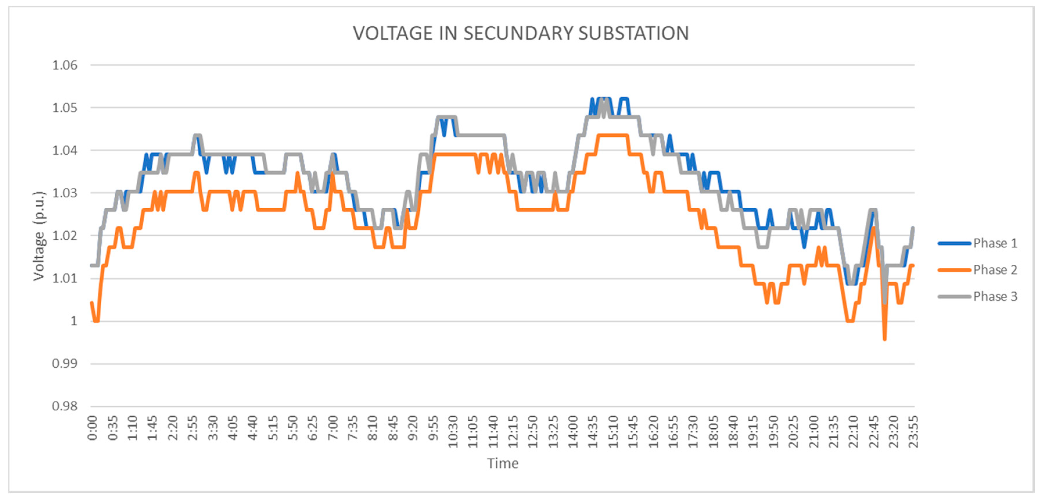
• Voltage profile in the transformer LV side of the selected day.
• Irradiation for PVs generation.

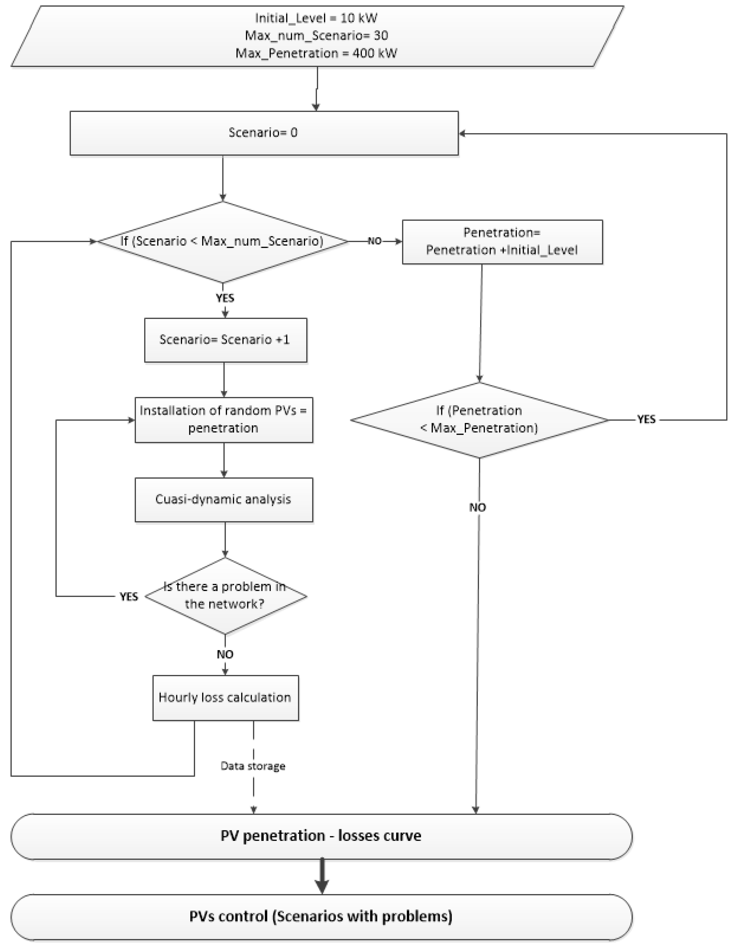
Next, the methodology to obtain the optimal distributed photovoltaic penetration is detailed. This analysis consists in increasing the photovoltaic penetration with steps of 10 kW, to reach the maximum level of PV penetration that could be installed by the clients randomly. In the Figure 1, it is shown a flow chart of the methodology to apply. The first step of the flowchart is to define different variables:

(a)

maximum number of scenarios for each level of penetration (Max_num_scenarios). For this study 30 scenarios have been chosen.

(b)

maximum penetration level (Max_Penetration). For this study 400 kW,

(c)

the minimum level of penetration (Install_level). For this study it starts with 10 kW.

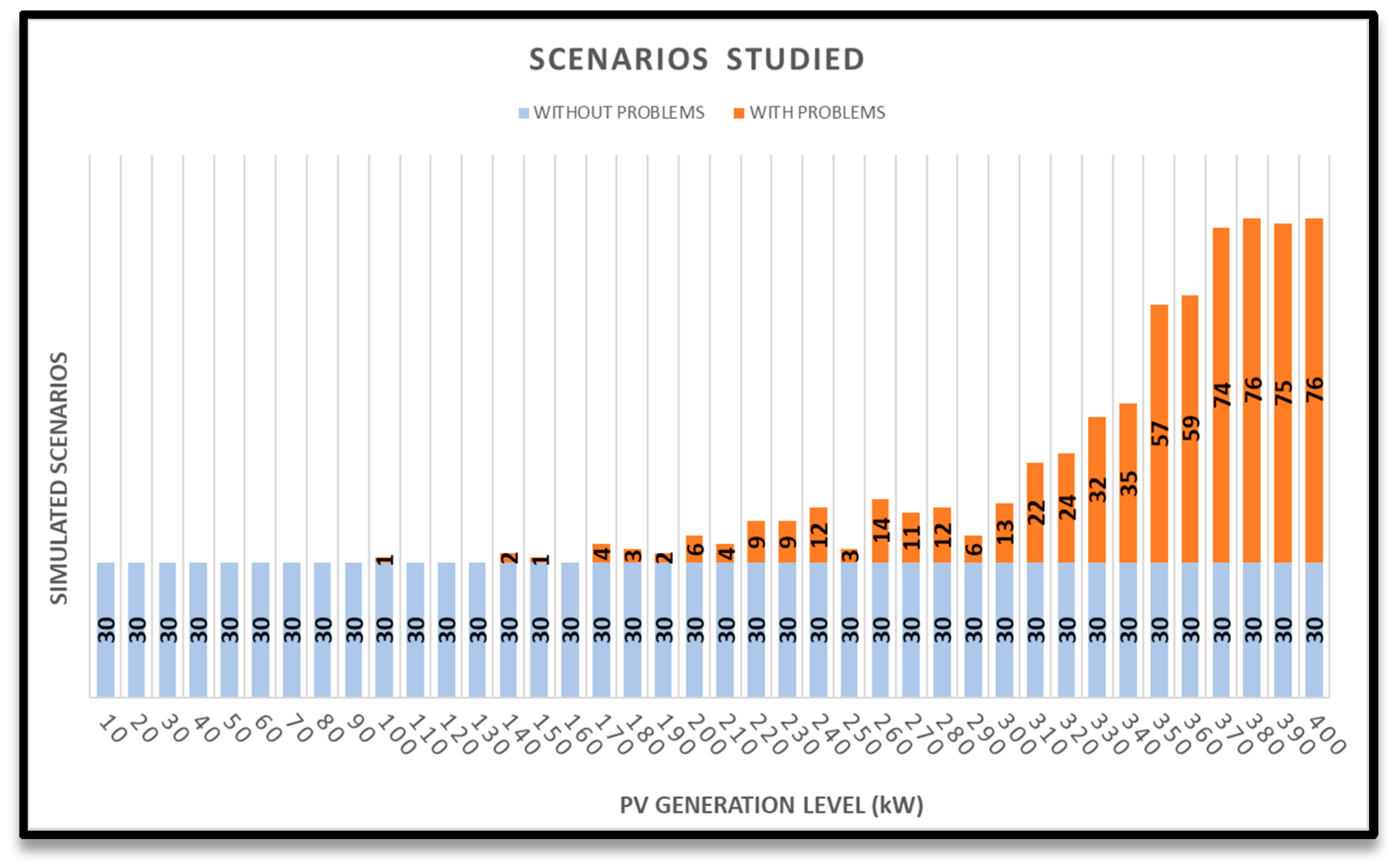
After defining the model parameters, the scenario counter is initialized (Scenario = 0). This variable is a counter increase (scenario = scenario + 1) until reaching 30 scenarios at each level of penetration. These 30 scenarios locate PV facilities uniform distribution in the network at existing customer connections, applying a Monte Carlo approach. The total power installed with PVs is set as the level of penetration. The size of each PV system is assumed to be equal to the customer’s contracted power and the phase to which it is connected. The total PV power installed is defined by the level of penetration. After completing all scenarios, penetration level is increased by 10 kW. This process is repeated until maximum penetration level is reached.

Networks should not have congestion problems or voltage deviations. Limits are set by each facility. In this case it is Grupo Cuerva that stablishes that voltage limits are 1.07 p.u. and 0.93 p.u., while the congestion limit of lines and transformer is 100%. In order to verify if there are any problems of congestion or voltage deviations, a quasi-dynamic study is executed each scenario, which consists in a power flow for each hour of a day.

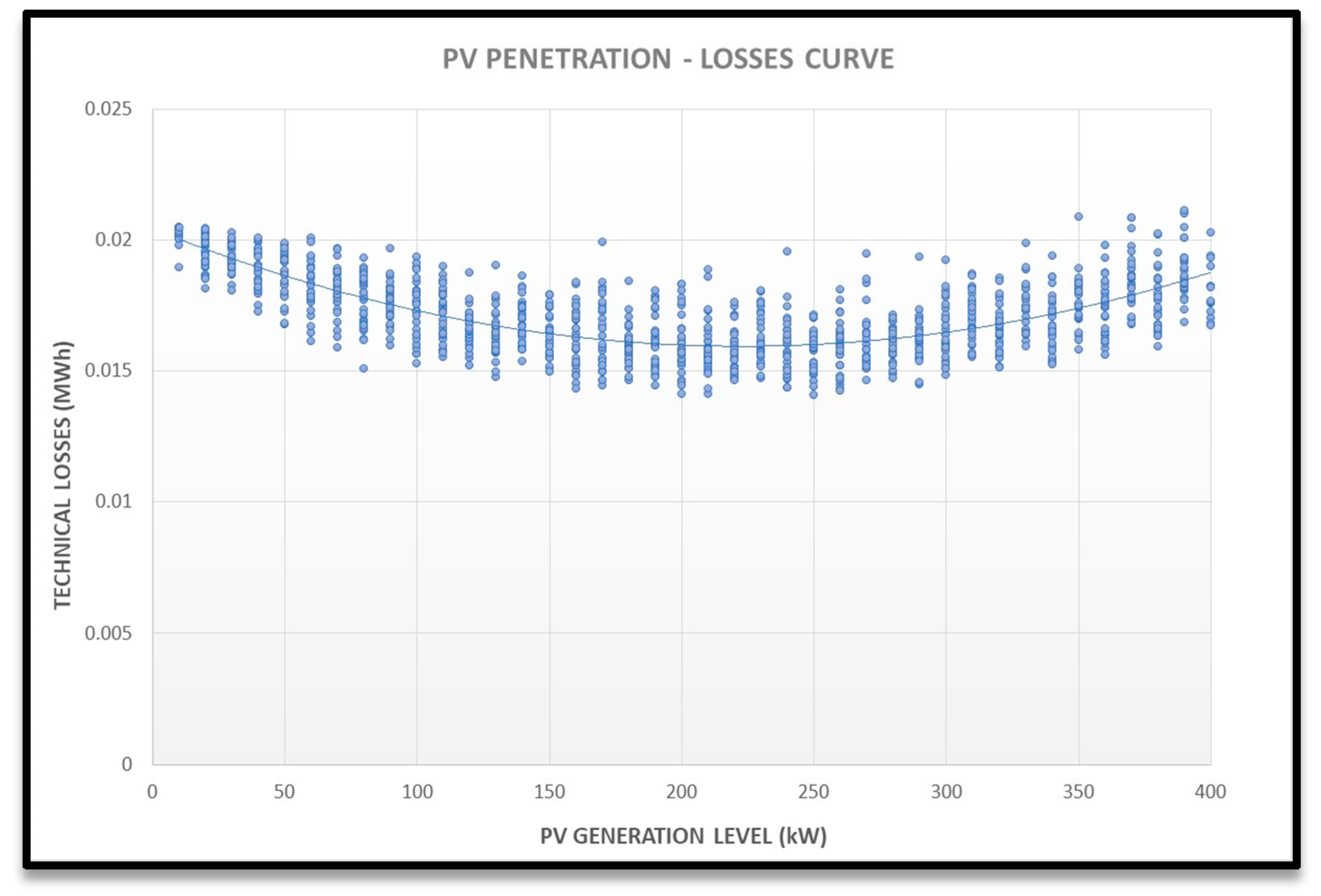
If no problems are detected, total losses are calculated and stored for each of the 24 h. Once there are 30 valid scenarios, the penetration of PVs is increased (Penetration = Penetration + 10 kW) until the maximum penetration is reached (Max_Penetration). After that, the curve “PV penetration-losses” is obtained. Finally, the optimal PV penetration level is derived from the minimum of the PV penetration-loss curve. According to the model definition, network losses decrease with increasing PV penetration until a certain level, where losses start to increase again.

After obtaining the optimal penetration value that minimizes systems losses, ten random uses cases are created with the optimal renewable penetration (240 kW), this choice is based on the study made to obtain the minimum losses in the system. The ten use cases are created with different PVs location (more information about the network topology in Appendix B). These ten use cases include congestion or voltage deviations. The control strategies are then evaluated in terms of ability to solve voltage problems caused by distributed PV generation. The controls tested are:

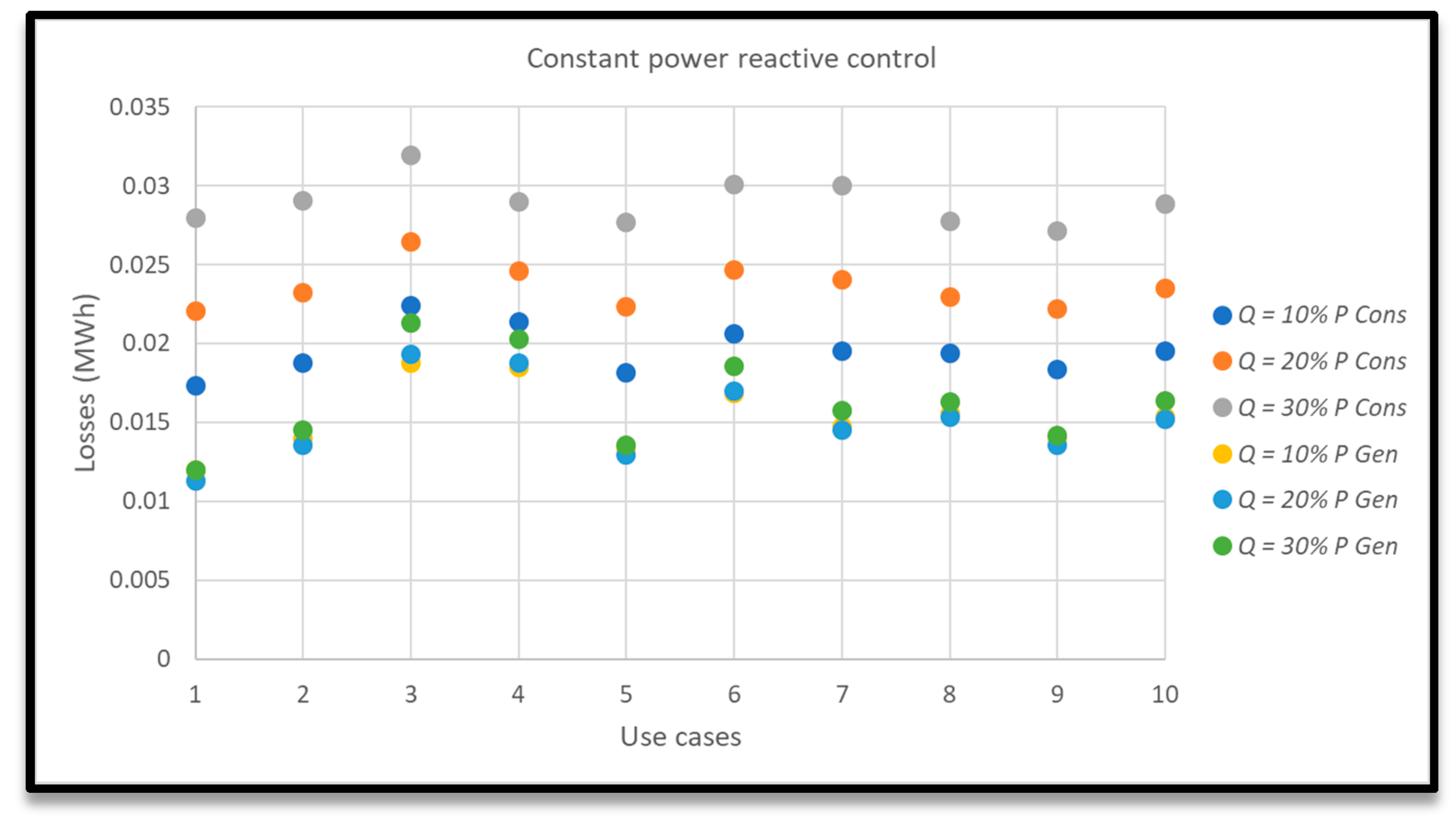
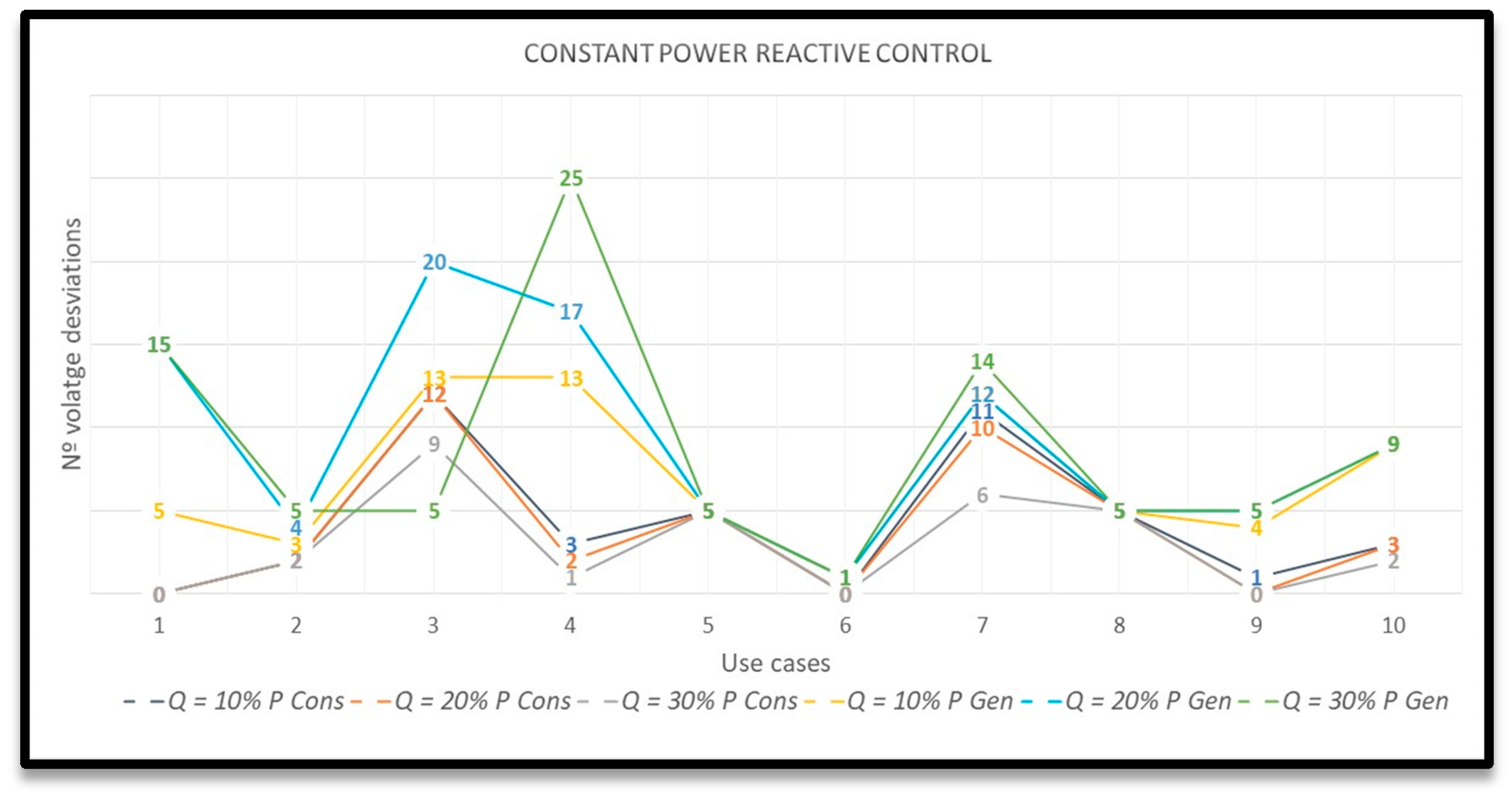
• Constant power reactive control (Q = constant): PVs consume or generate reactive power regardless of the active power installed. An amount of reactive power to be consumed or generated must be set. In order to evaluate efficiently this control strategy, six different values for Q are studied:

  ○

  Consumption of 10% active power PVs (Q = 10% P)

  ○

  Consumption of 20% active power PVs (Q = 20% P)

  ○

  Consumption of 30% active power PVs (Q = 30% P)

  ○

  Generation of 10% active power PVs (Q = 10% P)

  ○

  Generation of 10% active power PVs (Q = 20% P)

  ○

  Generation of 10% active power PVs (Q = 30% P)

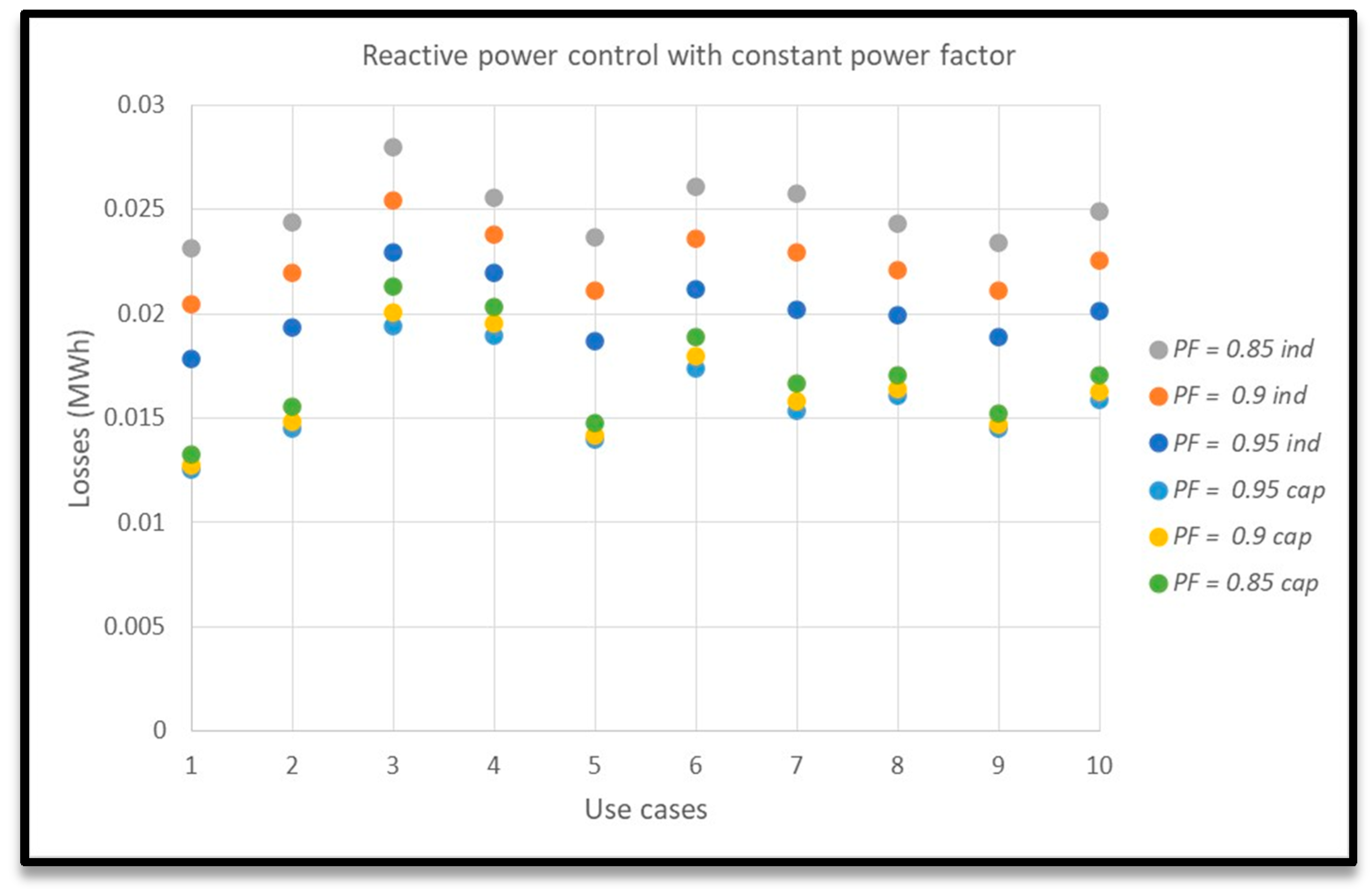
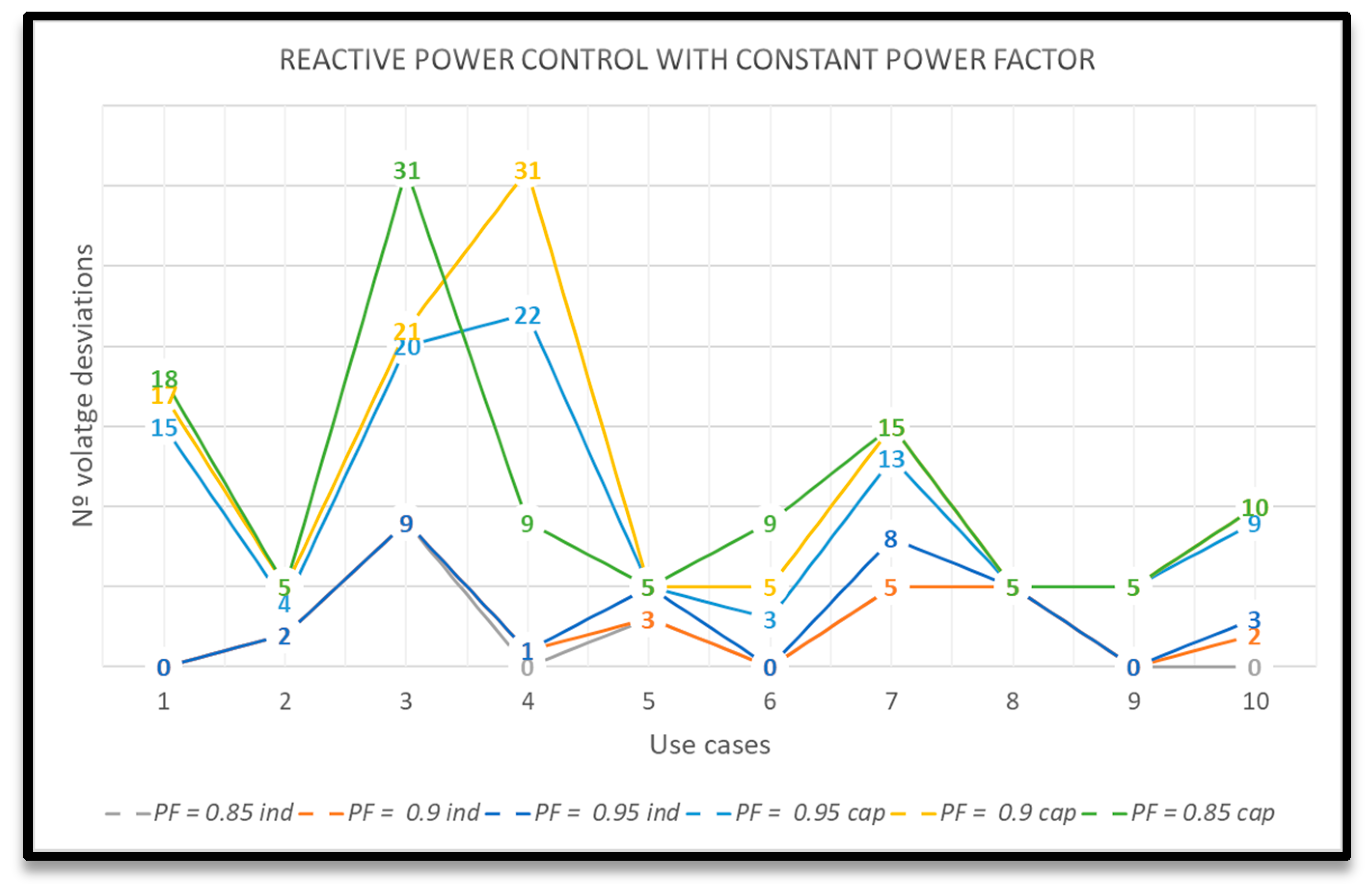
• Reactive power control with constant power factor (PF = constant): The power factor of PVs is set as a constant. To evaluate this control strategy, six PF values are considered indicating if it has inductive or capacitive characteristic (to consume or to generate, respectively):

  ○

  PF = 0.95 inductive

  ○

  PF = 0.95 capacitive

  ○

  PF = 0.9 inductive

  ○

  PF = 0.9 capacitive

  ○

  PF = 0.85 inductive

  ○

  PF = 0.85 capacitive

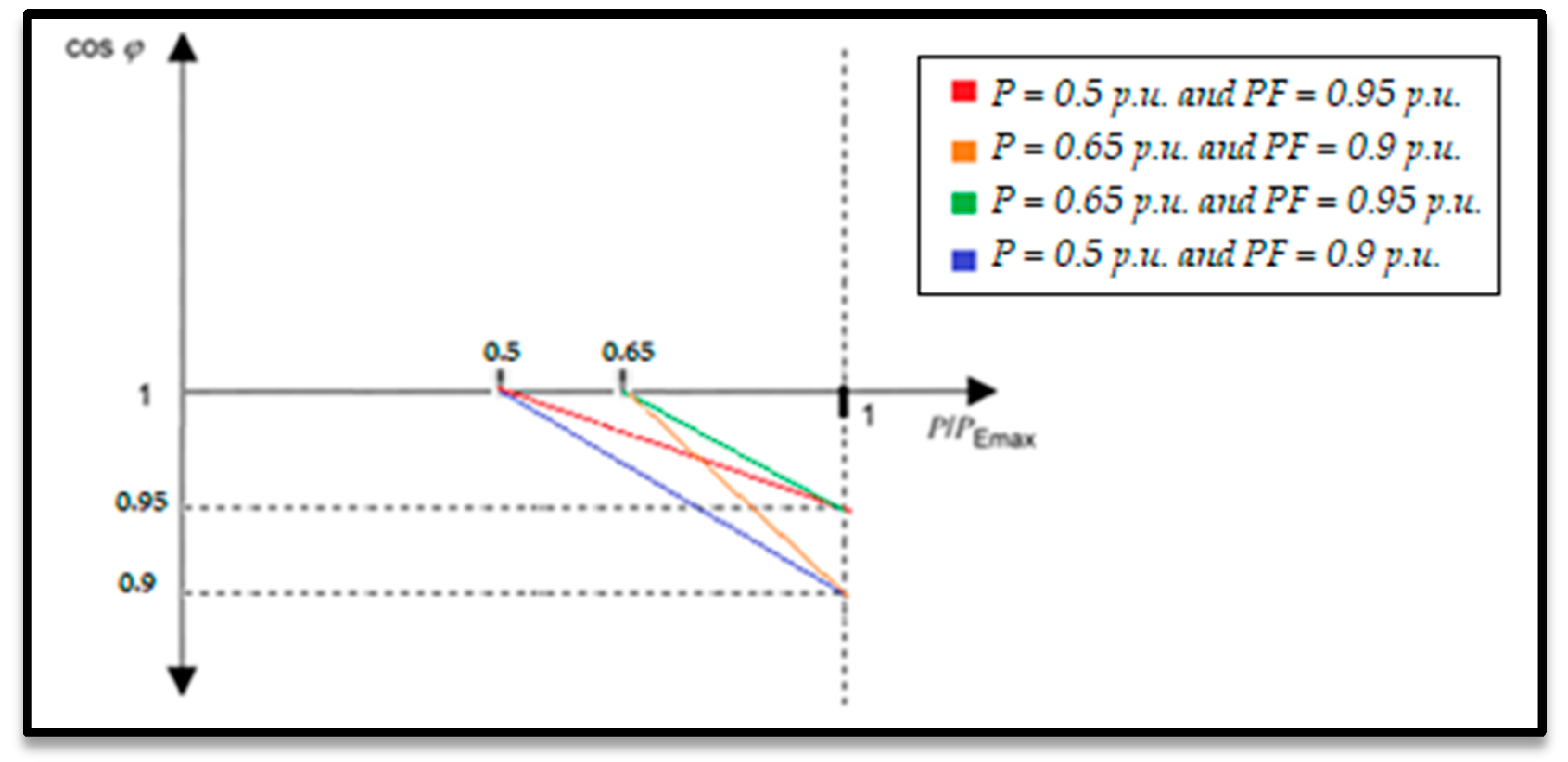
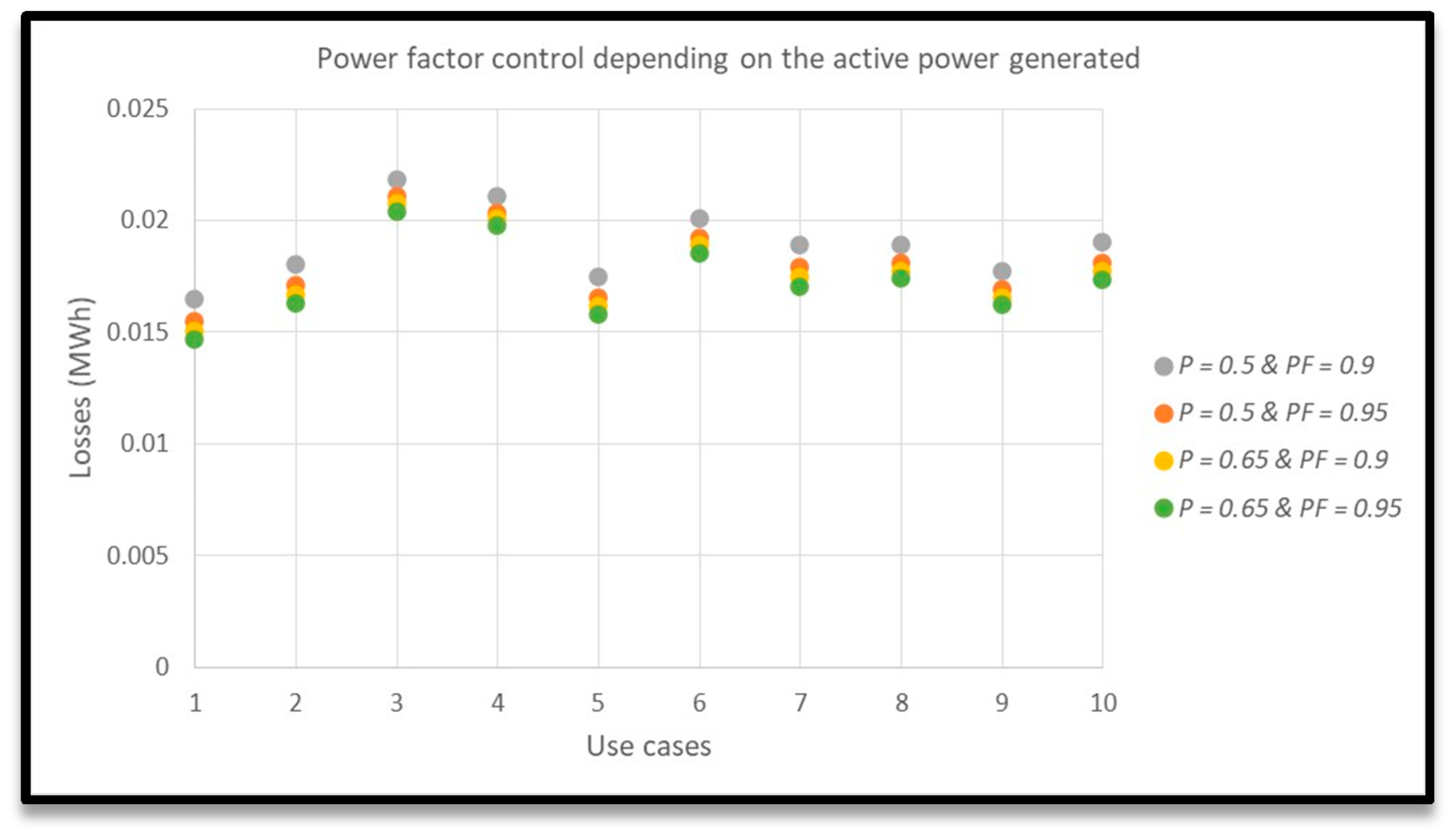
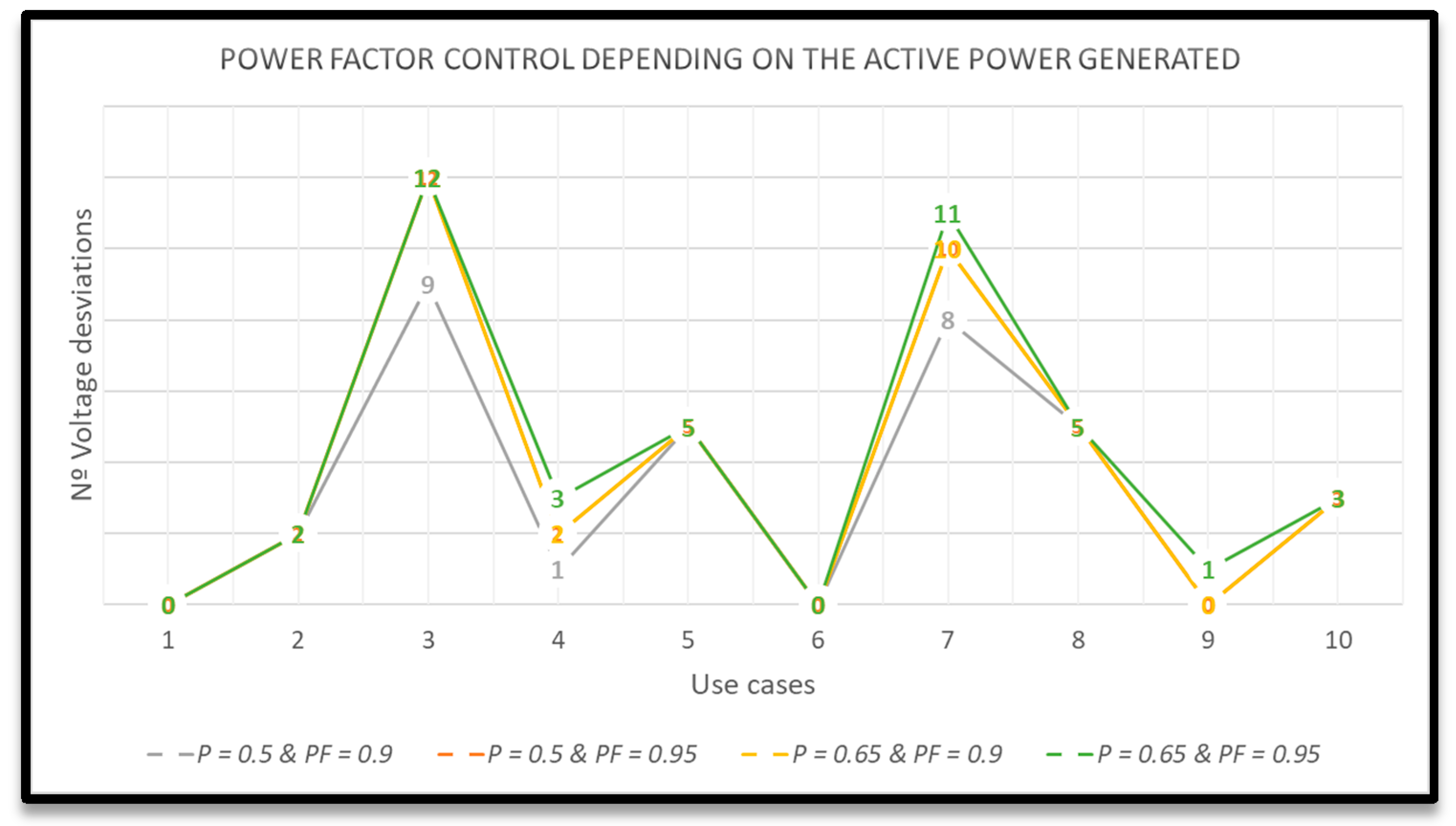
• Power factor control depending on the active power generated (PF = f(P)) [26]: PVs consume reactive power as a function of the active power generated at each moment. In this case the power factor depends on the active power generation. For this control strategy, two parameters are defined: (1) the minimum active power, that indicates which is the value where reactive power consumption starts; (2) the minimum value of the power factor.
  Figure 2 shows the PF variation curve used to set control strategies such as:

  ○

  P = 0.5 p.u. and PF = 0.9

  ○

  P = 0.5 p.u. and PF = 0.95

  ○

  P = 0.65 p.u. and PF = 0.9

  ○

  P = 0.65 p.u. and PF = 0.95

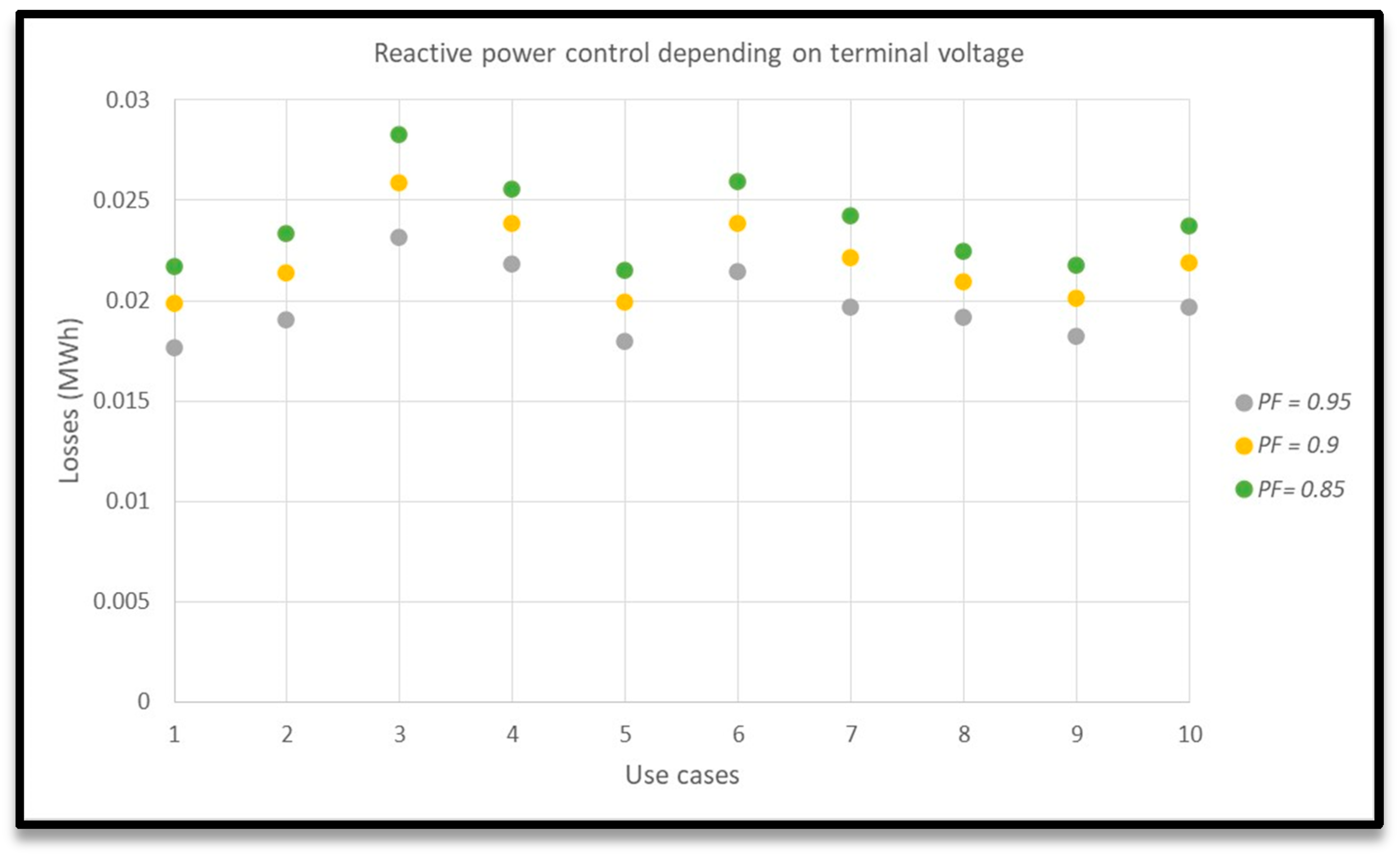
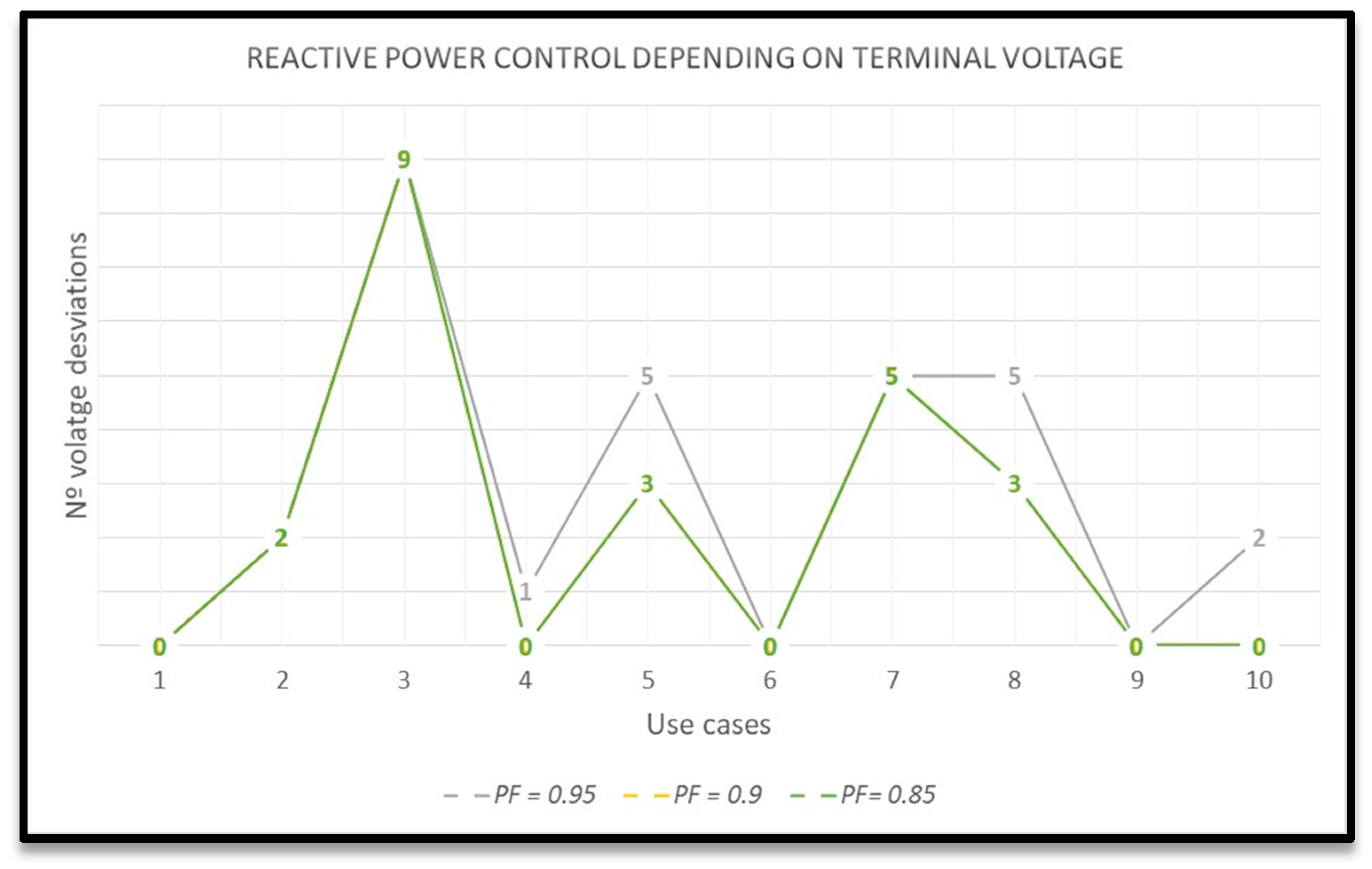
• Reactive power control depending on terminal voltage (Q = f(U)): PVs consume or generate enough reactive power to ensure that the grid terminals are within the permitted range. If the voltage is below a marked limit (i.e., 0.98 p.u.), the PV generates reactive power; and if the voltage is above a marked limit (i.e., 1.02 p.u.), the PV consumes reactive power. The maximum reactive power generated is reached when the voltage is 0.95 p.u. and the maximum reactive power consumed is reached when the voltage is 1.05 p.u. The three strategies implemented in this control are:

  ○

  PF = 0.95

  ○

  PF = 0.9

  ○

  PF = 0.85

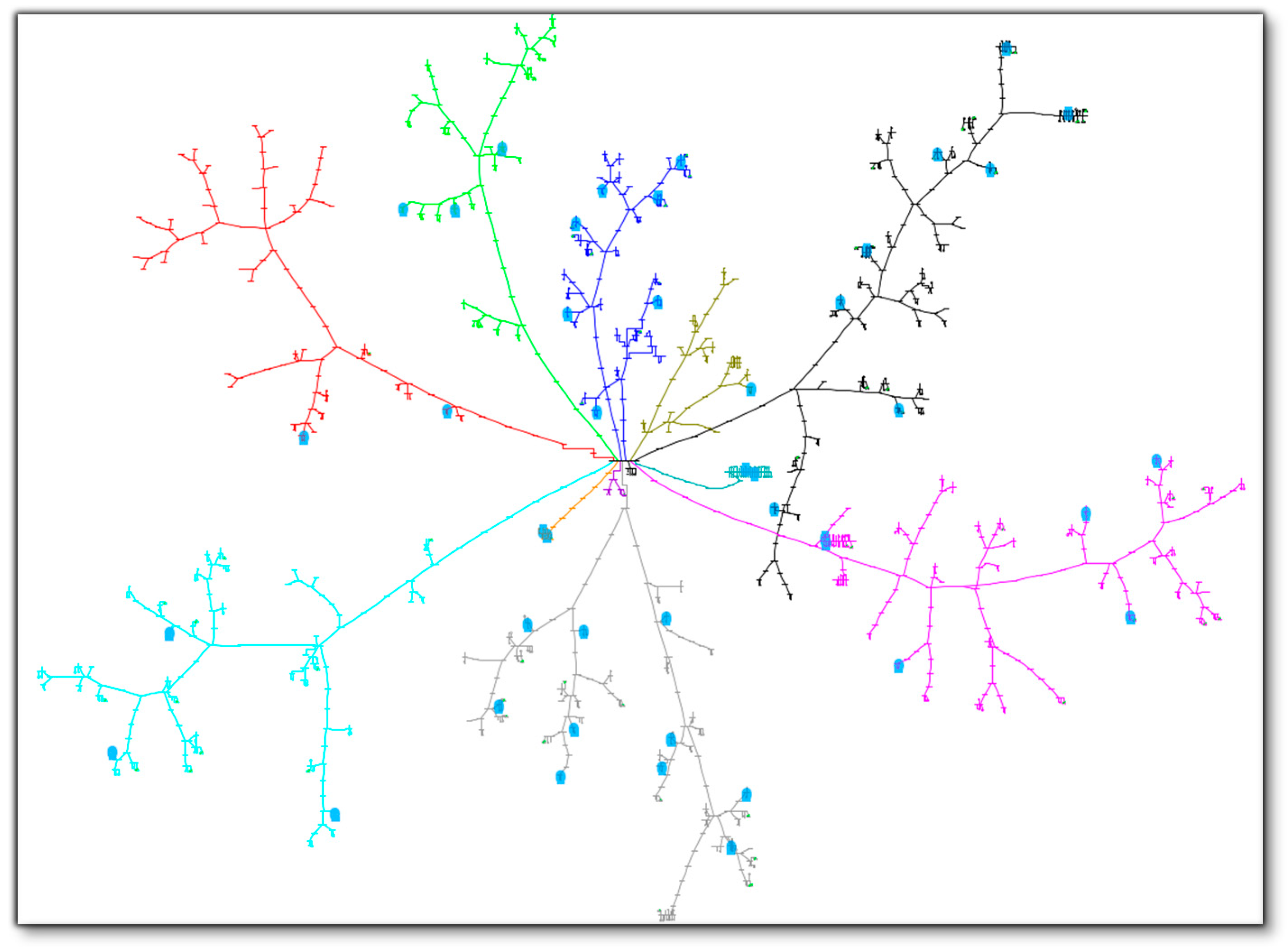
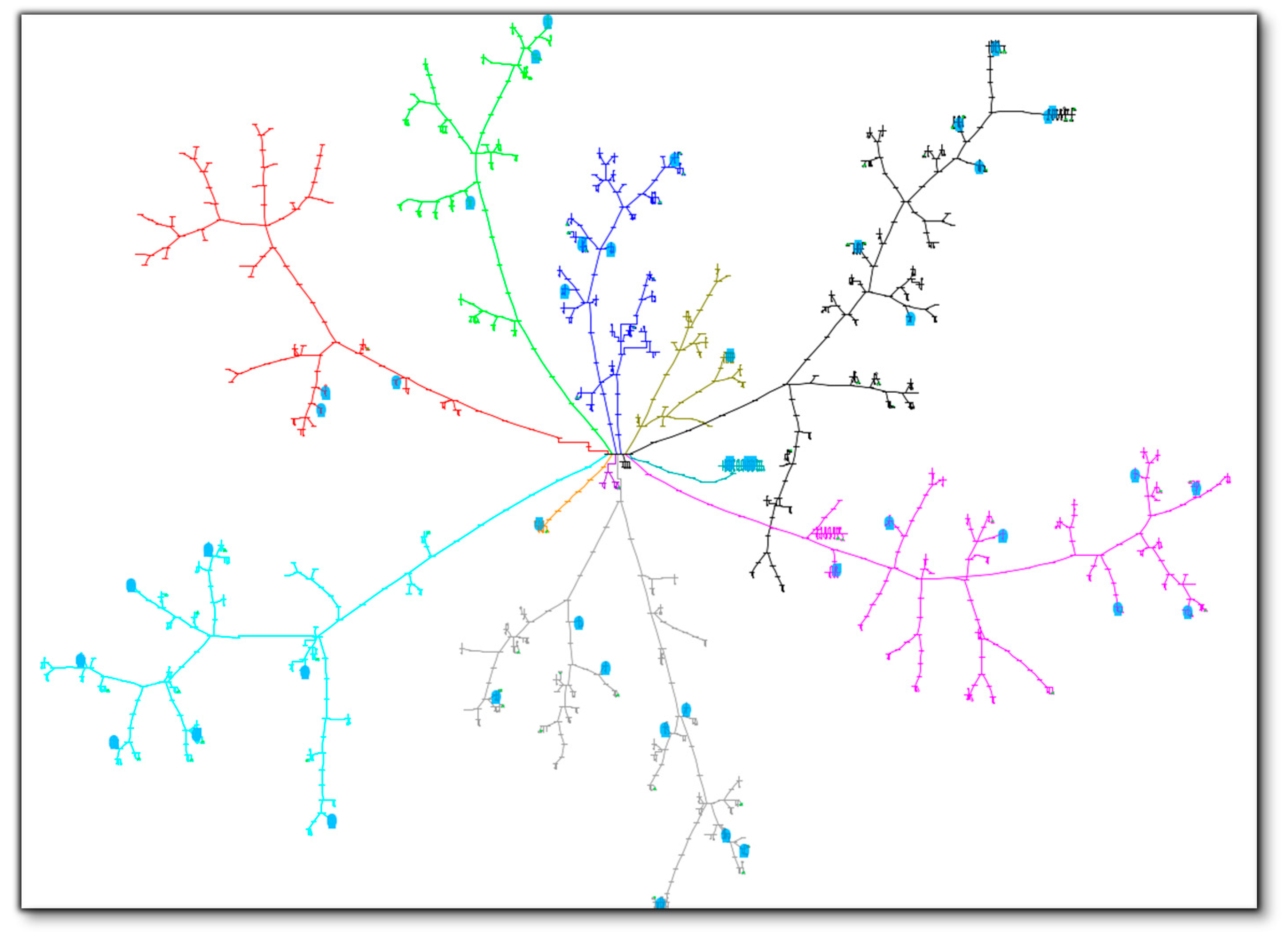
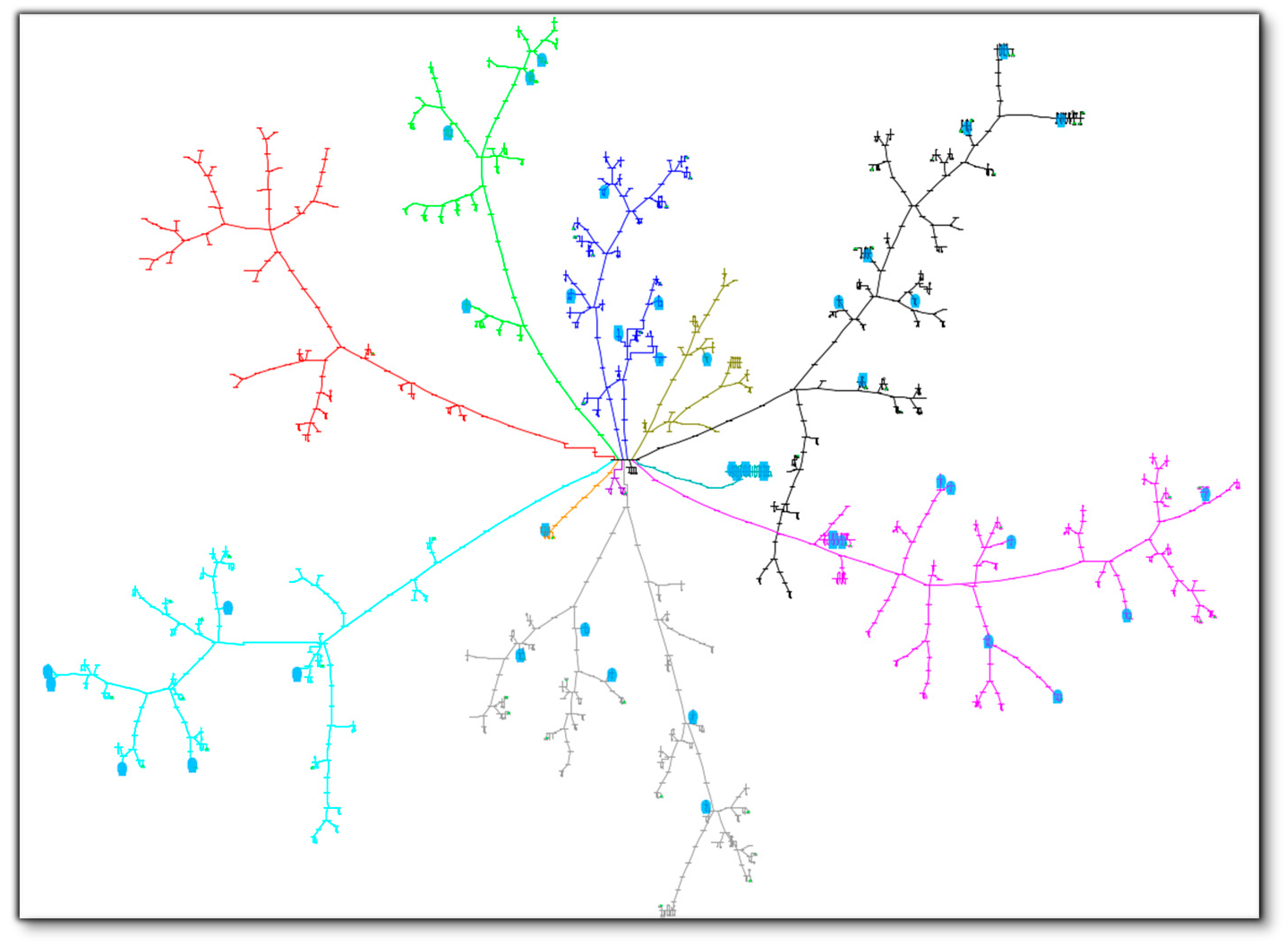
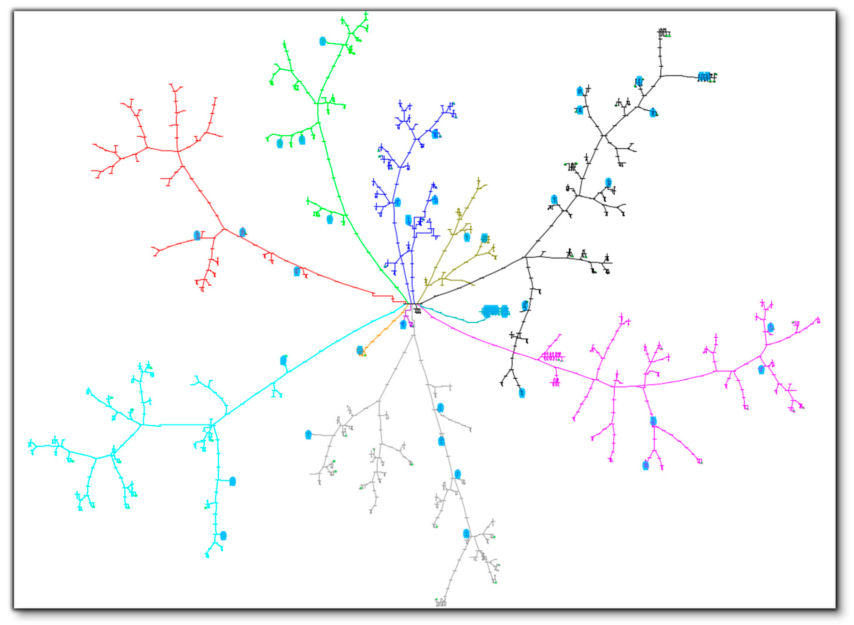
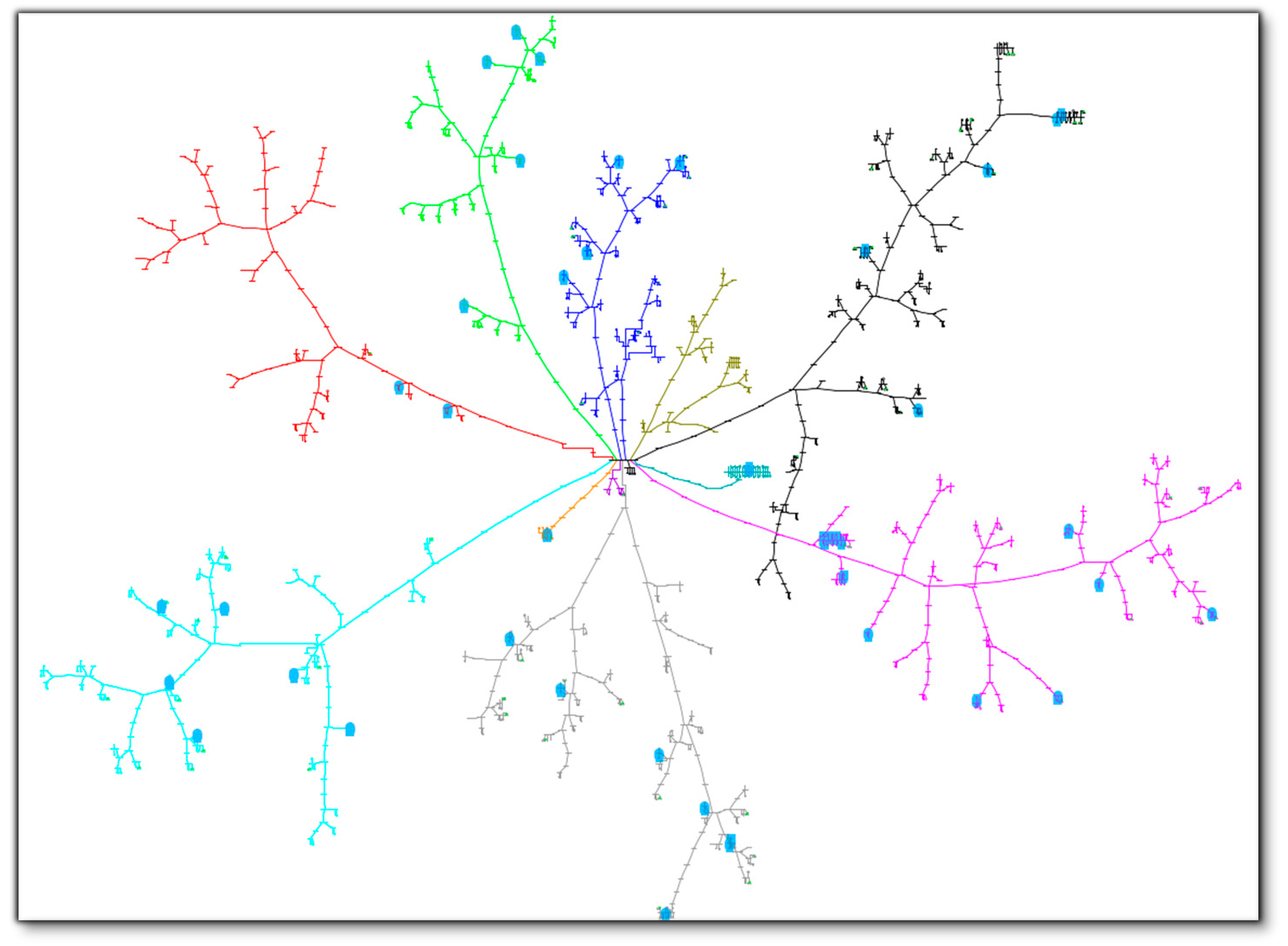
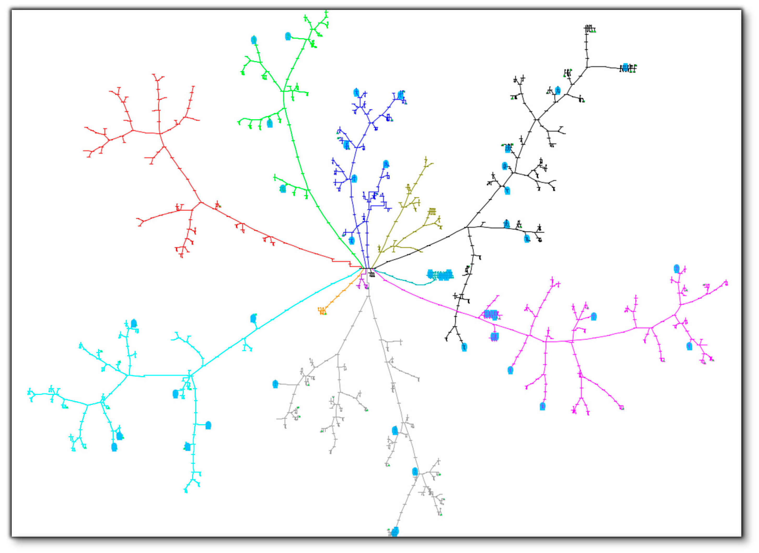
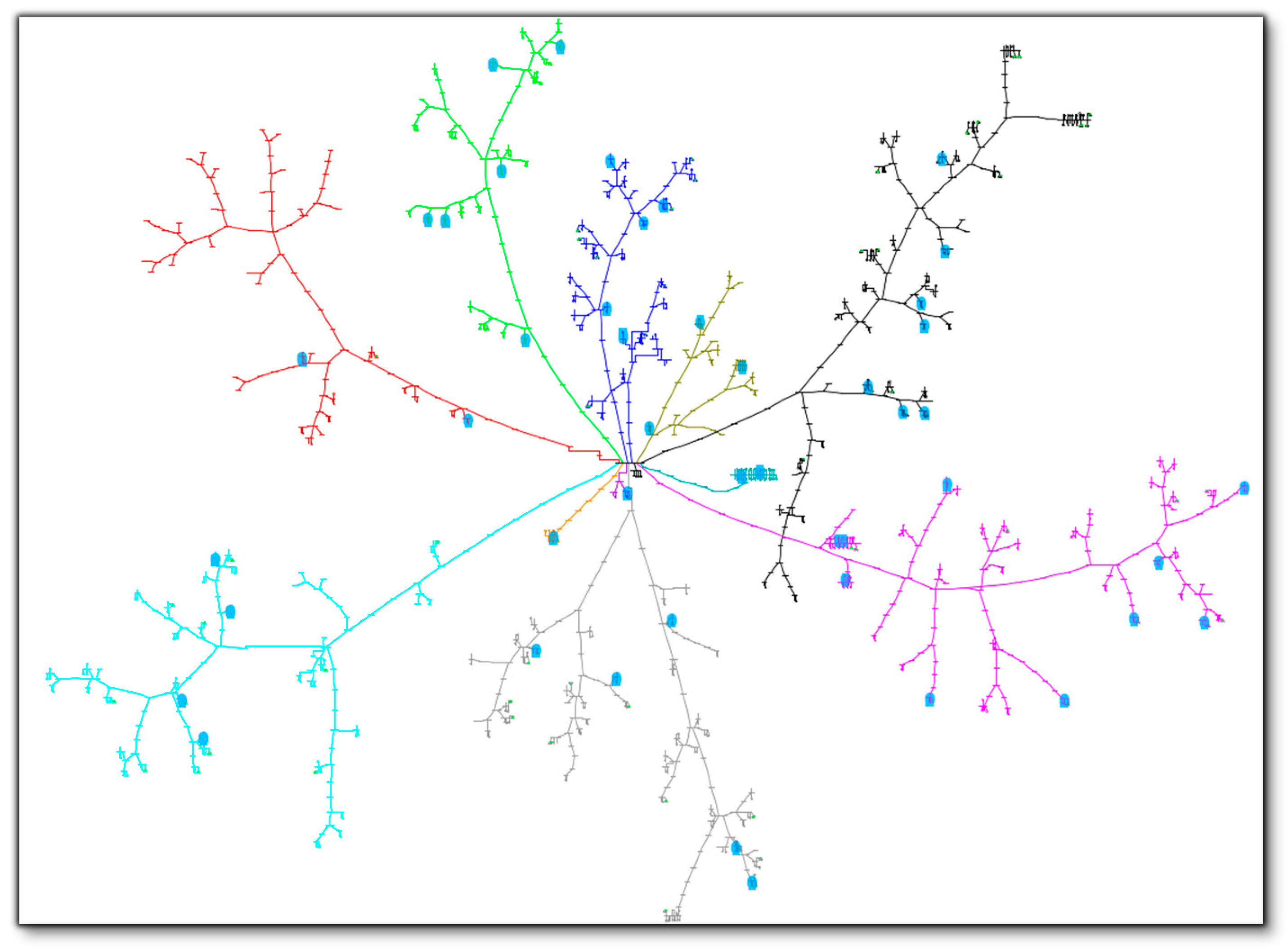
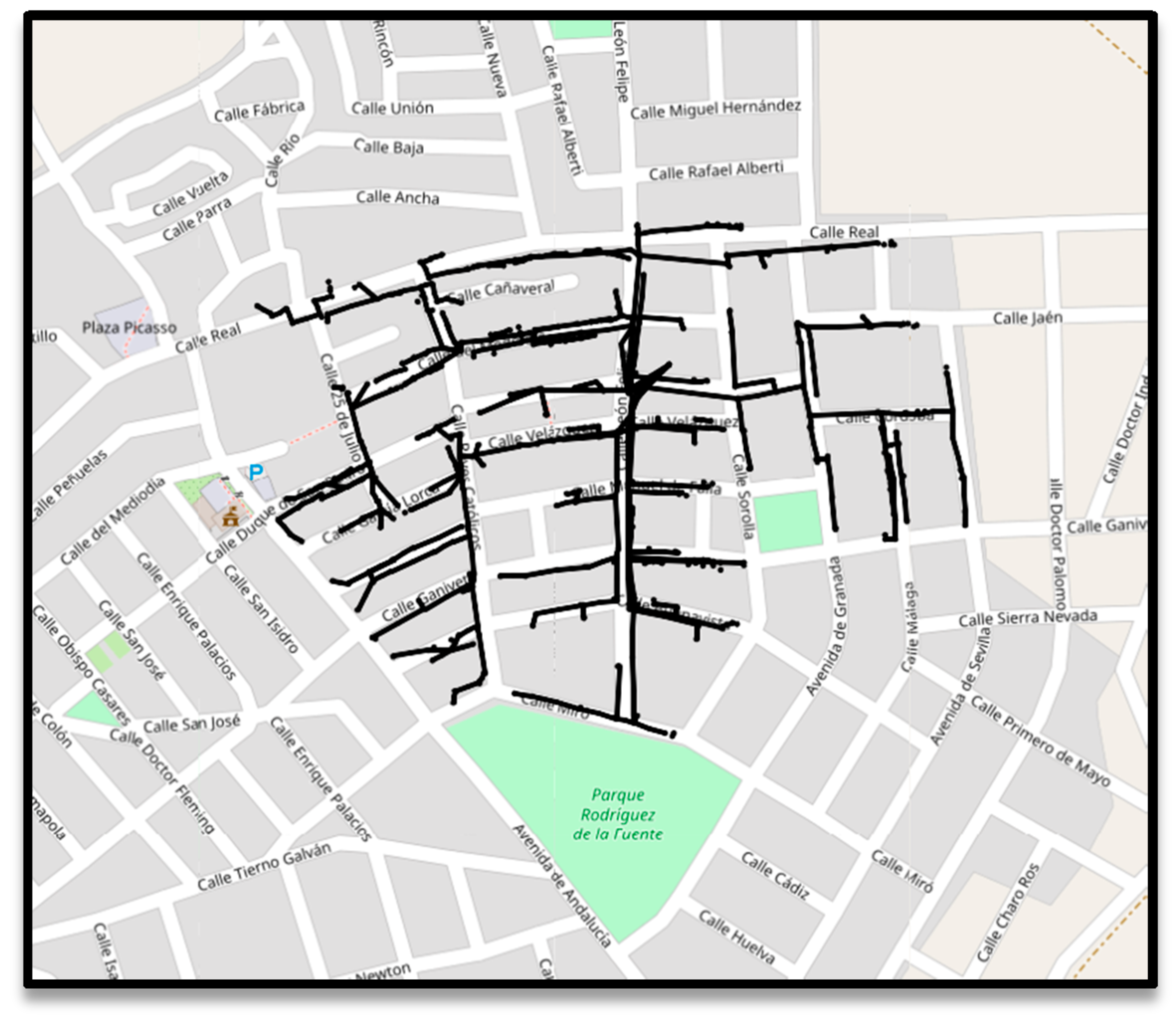
In order to test this methodology, a network model has been developed in PowerFactory DIgSILENT. A real model provided by Grupo Cuerva has been chosen, this real model is a district of a rural town. This model contains 266 consumers, from which 45 have a three-phase connection and 221 single-phase. The total installed power of all customer is 1, 320 MW approximately. This network is divided in 11 feeders (Figure A1 in Appendix A, each of the feeders is indicated in different colours) which have different lengths and different numbers of consumers. Figure 3 shows the LV network topology (More information about the network topology in Appendix A).

3. Results

The first part of this section provides the results of the study of optimal PV penetration and in the second part results from the different use cases are presented for each control strategy.

3.1. Optimal PV Penetration

As explained in Section 2, a method has been developed to obtain the optimum value (minimum losses in the LV network) of distributed PV penetration within a LV network, where PV systems are associated by Monte Carlo method to consumers within the LV grid.

For this purpose, in each level of penetration (10 kW, 20 kW…) until the maximum is reached (Max_Penetration), 30 scenarios are carried out in which Monte Carlo distributed generation is installed, that is, for each level of penetration 30 different scenarios will be obtained. For each of these scenarios a quasi-dynamic study (load flow for each hour) is carried out, allowing to obtain the value of the losses.

Each blue point in the Figure 4 represents the losses of scenario (total losses in the grid) in each PV penetration level, In other words, each level of penetration (PV generation) in Figure 4 has 30 blue points that represent the losses of each of the 30 scenarios (30 scenarios are defined as Max_num_scenarios in Figure 1, i.e., the 30 scenarios for each level of penetration in which losses are calculated). The tendency line that occurs between the different scenarios is the line that occurs when connecting the average points of losses of each level of penetration (PV generation).

Figure 4 confirms the expected effect, that distributed PV reduces total losses until certain penetration level and further increasing of PV installations increases also grid losses. The Monte Carlo method also reveals important differences depending on the actual distribution of the PV system within the grid.

As mentioned before, the increase of distributed PV generation may create problems in the network, such as voltage deviations (U > 1.07 p.u. or U < 0.93 p.u.) and congestions. One of the main issues is overvoltage as PV production may produce inverse power flows which increase voltage.

Figure 5 shows, in orange, the scenarios with problems in the network (congestion and/or voltage deviations) that have been obtained by Monte Carlo method, while trying to reach the 30 scenarios (30 scenarios are defined as Max_num_scenarios in Figure 1, i.e., the 30 scenarios for each level of penetration in which losses are calculated), without problems (blue).

As it can be seen in Figure 5, as distributed PV generation increases, more scenarios were found with problems of voltage deviations, which complicated the finding of the 30 scenarios without voltage deviations. For example, in the scenario with a penetration of 240 kW of distributed PV, 12 scenarios with grid problems have been obtained, this means that to find 30 scenarios without problems, 42 scenarios had to be analysed.

3.2. PV Control

In the following paragraphs, the control strategies explained in Section 2 are compared identifying the advantages and disadvantages of each control. To highlight the advantages and disadvantages of each option, three indicators have been used:

• Losses
• Voltage deviations (undervoltage and overvoltage)
• Congestions

To test each of the controls, ten use cases are created with different PV locations (see Appendix A for the locations of the PVs in each use case) but all of them with the same penetration 240 kW (total installed power for the PVs). In each of the use cases, a quasi-dynamic study (hourly load flow) will be performed over the period of one day in which the three indicators mentioned above will be calculated.

3.2.1. Constant Power Reactive Control

As explained in Section 2, the constant reactive power control consumes or generates the reactive power according to the value of the active power. Six values for reactive power have been considered (10, 20 and 30% of active power, capacitive and inductive)

The results obtained for these six control strategies in terms of losses (first indicator) can be seen in Figure 6. Figure 6 shows that the lowest values of losses are obtained when reactive power is being generated, since in all use cases, the lowest losses are obtained when the reactive power generated is 20% of the active power. This is because the reactive power is consumed by the loads and the reactive power transported by the network is minimized. While it is consumed, the highest losses are obtained in all use cases (grey points).

The second key indicator in this analysis is voltage deviation. In this case, no undervoltage event happened but overvoltage events occur. These overvoltage events are visualized in Figure 7.

When generating more reactive power (green and blue lines in Figure 7) there are more overvoltage events than when reactive power is consumed (grey line in Figure 7). For example, in use case 4, when reactive power is generated at 30% of active power, there are 25 overvoltage events in the network. However, if the reactive power is consumed at 30% of the active power, only one overvoltage event has been observed. Finally, the key congestion indicator has been analysed and the shows no congestion in any use case.

3.2.2. Reactive Power Control with Constant Power Factor

This control strategy considers a constant power factor, fixing reactive power proportional to active power generated. As mentioned in Section 2, six different PF levels have been considered (0.85, 0.9 and 0.95 inductive and capacitive).

The first indicator analysed is the losses, the results obtained for each use case can be seen in Figure 8. General conclusions are very similar to the first control strategy, where capacitive power factors are leading to lowest losses.

As can be seen in Figure 9, results regarding overvoltages are also very similar to the first control strategy with fixed reactive power control. In comparison, a slightly higher number of overvoltage events are observed for fixed PF control. This effect can be explained due to the fact that reactive power is highest when active power peaks, which are the hours where reversed power flows can be observed.

Finally, the result of this congestion indicator shows zero as there is no congestion in any of the use cases.

3.2.3. Power Factor Control Depending on Generated Active Power

The PV inverter consumes reactive power as a function of generated active power, the control parameters analysed are:

○

P = 0.5 p.u. and PF = 0.9

○

P = 0.5 p.u. and PF = 0.95

○

P = 0.65 p.u. and PF = 0.9

○

P = 0.65 p.u. and PF = 0.95

The results obtained evaluating the losses for this control strategy can be seen in Figure 10. As it can be seen in Figure 10, the loss values obtained applying the different control parameters are very close to each other. Thus, the effect on network losses is very limited.

Overvoltage events are shown in Figure 11. Similar to the other two control strategies, no under-voltage is observed. The number of overvoltage events in this case is considerably lower, which is mainly due to the fact that no capacitive reactive power has been considered.

In Figure 11, it can be seen that the control strategy of reactive power generation with 0.5 p.u. of active power and PF = 0.9 p.u., is the one where less overvoltage events are obtained. Therefore, if only the overvoltage events are considered, this would be the optimal strategy.

3.2.4. Reactive Power Control Depending on Terminal Voltage

With this strategy, PV facilities aim keeping terminal voltages within desired limits, adjusting reactive power accordingly withing a predefined range. In this case study, reactive power limits have been defined in terms of PF, considering 3 cases.

○

PF = 0.95 p.u.

○

PF = 0.9 p.u.

○

PF = 0.85 p.u.

The first key indicator to analyse is losses. Figure 12 shows network losses for this control strategy of PF = 0.95 p.u. (grey dots), PF = 0.9 p.u. (yellow dots) and PF = 0.85 p.u. (green dots).

Figure 12 shows that the lowest losses are obtained when the power factor is 0.95, i.e., when less reactive power is delivered per voltage level.

The number of overvoltage events is shown in Figure 13, where is becomes clear that with the lowest PF (0.85) limit, overvoltages can be reduced most. This is not surprising, as the more reactive power is allowed to be consumed, the higher is the effect on terminal voltages. Nevertheless, it should be highlighted here, that this reduction of overvoltages comes with the downside of increased network losses.

As happened in the previous control, in the use case there are no congestions and therefore the last key indicator, congestions, is zero.

3.2.5. Comparison of Control Strategies

In this section, all evaluated control strategies are compared regarding losses and overvoltages. Figure 14 shows a comparison of network losses. Each control has several points according to the different control strategies: 6 dots for Q constant represented by a blue dot in Figure 14, 6 for PF constant represented by red dots in Figure 14, 4 for PF = f(P) represented by green dots in Figure 14 and 3 for Q = f(U)) represented by yellow dots in Figure 14.

In the Figure 14, identifying the optimal control is difficult because there is no clear tendency in the controls. For example, in the constant value control of Q, a very small value of losses is observed if the reactive power is low and a very high value of losses if the reactive power consumed is high. The same situation occurs when the constant PF control is applied. However, the three dots (green dots in Figure 14) that define the PF = f(P) are close and the losses are small enough in order to select this control as optimal control.

Figure 15 shows the number of overvoltage events in each use case for each control strategy. In Figure 15 it can be seen the effectiveness of each control. It is represented by the number of terminals in overvoltage. The results show that Q = f(U) (yellow line Figure 15) is the most effective control as in all use cases has the lowest number of overvoltage events.

For the selection of the optimal control, it is necessary to take into account both key indicators (losses, voltage deviations) and to reach an agreement on which level of losses and overvoltage events are considered as valid. As a conclusion, the optimal controls would be Q = f(u) and PF = f(p) since they are the controls that cause the least overvoltage events and the loss values are sufficiently small.

4. Conclusions

In this paper, two main topics have been analysed: on the one hand, to propose a method to calculate the photovoltaic hosting capacity that minimizes system losses, and on the other, to evaluate different management techniques for solar PV inverters and their effect on the hosting capacity aforementioned

In a first step, optimal PV penetration levels have been derived using a Monte Carlos approach, considering optimal PV penetration when network losses are minimised, that is to say, the HC has been obtained in each node where self-consumption can be introduced, which minimizes the losses of the system.. This approach is very promising for planning purposes, if a detailed network model is available. Similar methods are proposed in the works of [11] or [25], however in this article the scope has been extended using real data from the smart meters, the installed PVs can be installed in single phase or three-phase (depending on the installation of the consumer), the size of the installed PV will depend on the contracted power of the consumer, with this it is possible to evaluate the effect of PV self-consumption in a distribution network. Some improvements can be proposed for future studies: (i) it has been used a standard day and it is proposed to use a whole year of smart meter data to evaluate the seasonal effect (autumn, spring, winter and summer), (ii) it has been assumed that PV facilities power is equal to the contracted power and it could be interesting modelling the variability of the installed PV facilities and for the last (iii) it will be evaluated other methods to expand the penetration of renewables such as distributes storage technologies and / or demand response policies, either through direct signals or through a local market flexibility.

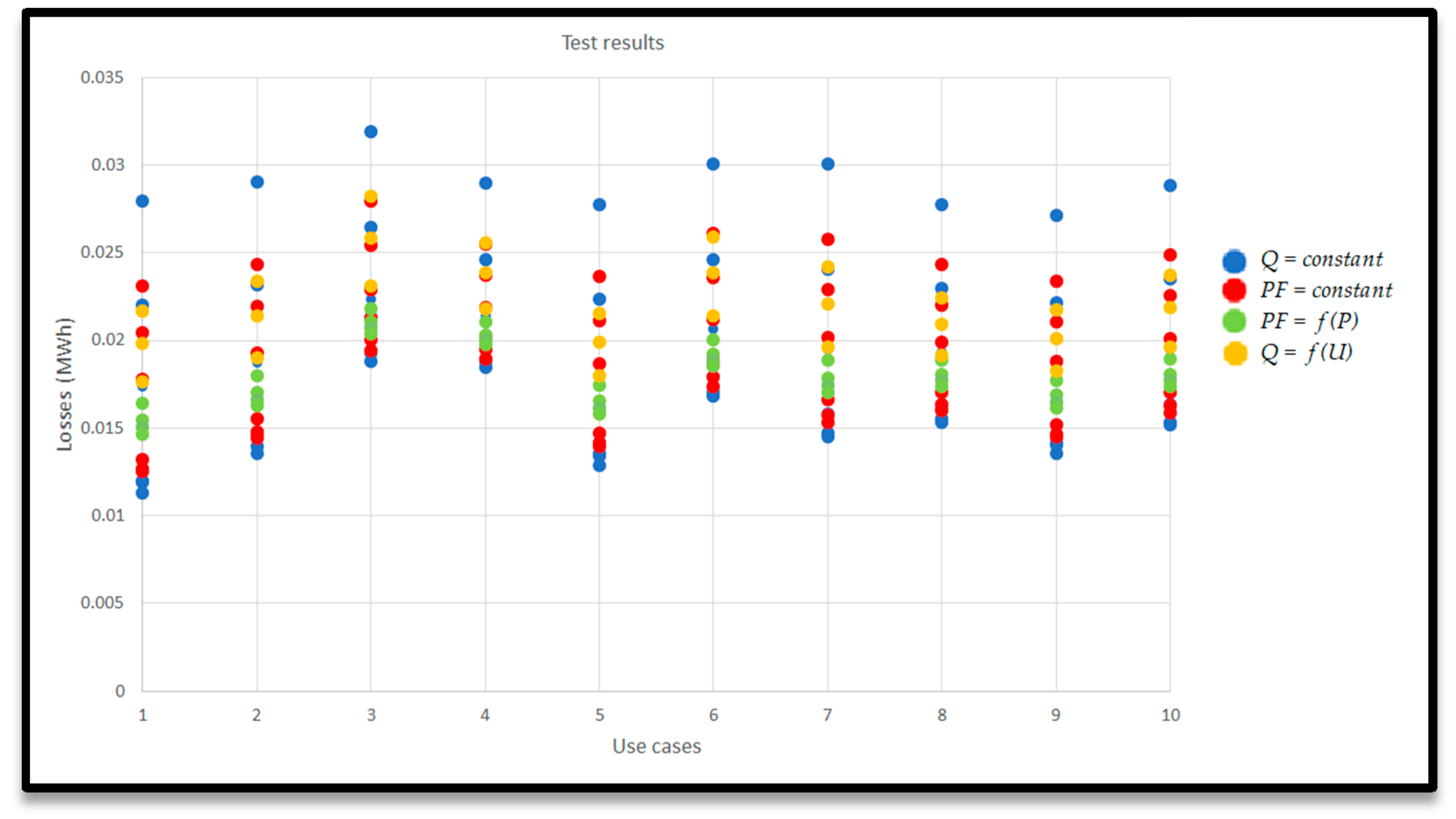
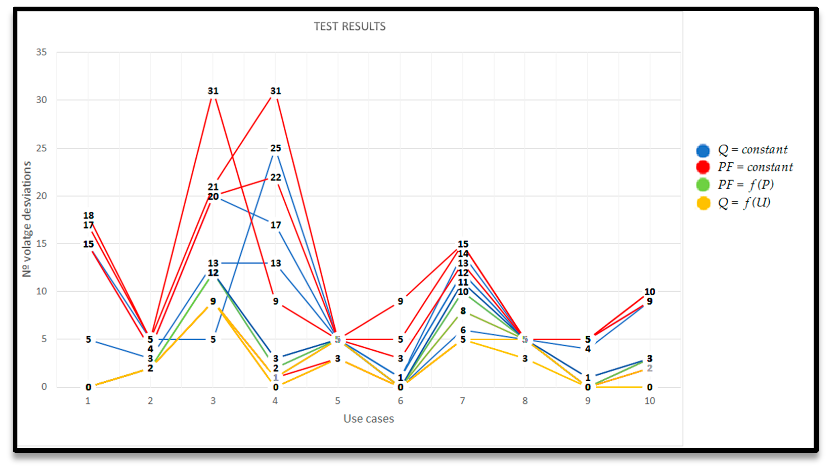
The second topic was dedicated to the evaluation of 4 different control strategies of solar PV inverters, considering the possibility of reactive power control to mitigate excessive voltage deviations. In addition, the effect on total network losses have been documented. Congestion problems were also expected, but were not observed in this case study, given the restrictive condition which limits installed solar PV power at consumer premises to their respective contracted power. The effectiveness of this limit could be demonstrated hereby.

In the tested grid, 240 kW of installed PV power has been found as the optimal penetration level in terms of technical losses. The 4 control strategies have been tested for this penetration level, and ten use cases were generated in which overvoltage occurred. Control strategies with constant reactive power or PF setpoints were outperformed by more dynamic approaches considering generated power to modify PF and terminal voltages to modify reactive power.

References

1. Mansouri, N.; Lashab, A.; Sera, D.; Guerrero, J.M.; Cherif, A. Large photovoltaic power plants integration: A review of challenges and solutions. Energies 2019, 12, 3798. [Google Scholar] [CrossRef] [Green Version]
2. Munkhchuluun, E.; Meegahapola, L. Impact of the Solar Photovoltaic (PV) Generation on Long-Term Voltage Stability of a Power Network. In Proceedings of the 2017 IEEE Innovative Smart Grid Technologies—Asia (ISGT–Asia), Auckland. 2017, pp. 1–6. Available online: https://ieeexplore.ieee.org/abstract/document/8378456/authors#authors (accessed on 20 April 2020).
3. Eguía, P.; Torres, E.; Etxegarai, A. Impact of Photovoltaic Self-consumption on Power Losses and Voltage Levels of MV Distribution Networks. 2017. Available online: https://ieeexplore.ieee.org/abstract/document/8260161 (accessed on 20 April 2020).
4. Tavakkoli, M.; Pouresmaeil, E.; Godina, R.; Vechiu, I.; Catalão, J.P. Optimal management of an energy storage unit in a PV-based microgrid integrating uncertainty and risk. Appl. Sci. 2019, 9, 169. [Google Scholar] [CrossRef] [Green Version]
5. Aziz, T.; Ketjoy, N. PV Penetration Limits in Low Voltage Networks and Voltage Variations. IEEE Access 2017, 5, 16784–16792. [Google Scholar] [CrossRef]
6. Patil, A.; Girgaonkar, R.; Musunuri, S.K. Impacts of Increasing Photovoltaic Penetration on Distribution Grid—Voltage Rise Case Study. In Proceedings of the 2014 International Conference on Advances in Green Energy, (ICAGE), Thiruvananthapuram, India, 17–18 December 2014; pp. 100–105. Available online: https://ieeexplore.ieee.org/abstract/document/7050150 (accessed on 20 April 2020).
7. Gandhi, O.; Kumar, D.S.; Rodriguez-Gallegos, C.; Srinivasan, D. Review of power system impacts at high PV penetration Part I: Factors limiting PV penetration. Solar Energy 2020, 1–21, In Press, Corrected Proof. Available online: https://www.sciencedirect.com/science/article/abs/pii/S0038092X20307118 (accessed on 20 April 2020).
8. Wajahat, M.; Khalid, H.A.; Bhutto, G.M.; Leth Bak, C. A Comparative Study into Enhancing the PV Penetration Limit of a LV CIGRE Residential Network with Distributed Grid-Tied Single-Phase PV Systems. Energies 2019, 12, 2964. [Google Scholar] [CrossRef] [Green Version]
9. Ul Abideen, M.Z.; Ellabban, O.; Al-Fagih, L. A review of the tools and methods for distribution networks’ hosting capacity calculation. Energies 2020, 13, 2758. [Google Scholar] [CrossRef]
10. Bollen, M.H.; Rönnberg, S.K. Hosting capacity of the power grid for renewable electricity production and new large consumption equipment. Energies 2017, 10, 1325. [Google Scholar] [CrossRef] [Green Version]
11. Klonari, V.; Toubeau, J.; Lobry, J.; Vallée, F. Photovoltaic integration in smart city power distribution: A probabilistic photovoltaic hosting capacity assessment based on smart metering data. In Proceedings of the 2016 5th International Conference on Smart Cities and Green ICT Systems (SMARTGREENS), Rome, Italy, 23–25 April 2016; pp. 1–13. [Google Scholar]
12. Mateo, C.; Frías, P.; Cossent, R.; Sonvilla, P.; Barth, B. Overcoming the barriers that hamper a large-scale integration of solar photovoltaic power generation in European distribution grids. Sol. Energy 2017, 153, 574–583. [Google Scholar] [CrossRef]
13. Yuan, J.; Weng, Y.; Tan, C.W. Quantifying Hosting Capacity for Rooftop PV System in LV Distribution Grids. 2019, pp. 1–10. Available online: https://arxiv.org/abs/1909.00864 (accessed on 20 April 2020).
14. Hong, B.; Li, Q.; Miao, W.; Yan, H.; Liu, J. Energy Storage Application in Improving Distribution Network’s Solar Photovoltaic (PV) Adoption Capability. Energy Procedia 2018, 145, 472–477. [Google Scholar] [CrossRef]
15. Denholm, P.; Margolis, R.M. Evaluating the limits of solar photovoltaics (PV) in electric power systems utilizing energy storage and other enabling technologies. Energy Policy 2007, 35, 4424–4433. [Google Scholar] [CrossRef]
16. Jeong, Y.C.; Lee, E.B.; Alleman, D. Reducing voltage volatility with step voltage regulators: A life-cycle cost analysis of Korean solar photovoltaic distributed generation. Energies 2019, 12, 652. [Google Scholar] [CrossRef] [Green Version]
17. Torres, I.C.; Negreiros, G.F.; Tiba, C. Theoretical and experimental study to determine voltage violation, reverse electric current and losses in prosumers connected to low-voltage power grid. Energies 2019, 12, 4568. [Google Scholar] [CrossRef] [Green Version]
18. Bremdal, B.A.; Mathisen, G.; Degefa, M.Z. Flexibility offered to the distribution grid from households with a photovoltaic panel on their roof. In Proceedings of the 2018 IEEE International Energy Conference (ENERGYCON), Limassol, Cyprus, 3–7 June 2018; pp. 1–6. Available online: https://ieeexplore.ieee.org/abstract/document/8398848 (accessed on 20 April 2020).
19. PARITY Project. Available online: https://parity-h2020.eu/ (accessed on 20 April 2020).
20. FLEXCoop Project. Available online: http://www.flexcoop.eu/ (accessed on 20 April 2020).
21. Mateo, C.; Cossent, R.; Gómez, T.; Prettico, G.; Frías, P.; Fulli, G.; Meletiou, A.; Postigo, F. Impact of solar PV self-consumption policies on distribution networks and regulatory implications. Sol. Energy 2018, 176, 62–72. [Google Scholar] [CrossRef]
22. Sauhats, A.; Zemite, L.; Petrichenko, L.; Moshkin, I.; Jasevics, A. Estimating the economic impacts of net metering schemes for residential PV systems with profiling of power demand, generation, and market prices. Energies 2018, 11, 3222. [Google Scholar] [CrossRef] [Green Version]
23. Ren, B.; Zhang, M.; An, S.; Sun, X. Local Control Strategy of PV Inverters for Overvoltage Prevention in Low Voltage Feeder. In Proceedings of the 2016 IEEE 11th Conference on Industrial Electronics and Applications (ICIEA), Hefei, China, 5–7 June 2016; pp. 2071–2075. [Google Scholar]
24. Zhang, Y.; Wang, X. PV reactive voltage regional autonomy control strategy for Q (U) improvement in distribution network. In Proceedings of the 2019 4th International Conference on Intelligent Green Building and Smart Grid (IGBSG), Yi-chang, China, 6–9 September 2019; pp. 497–501. [Google Scholar]
25. Duwadi, K.; Ingalalli, A.; Hansen, T.M. Monte Carlo Analysis of High Penetration Residential Solar Voltage Impacts using High Performance Computing. In Proceedings of the 2019 IEEE International Conference on Electro Information Technology (EIT), Brookings, SD, USA, 20–22 May 2019; pp. 1–6. [Google Scholar]
26. German Standard VDE-AR-N 4105. Available online: https://www.vde.com/en/fnn/topics/technical-connection-rules/power-generating-plants (accessed on 20 April 2020).
Figure 1. Methodology to obtain the optimal PV penetration level.
Energies 13 04347 g001
Figure 2. PF variation curve depending on the active power generated.
Energies 13 04347 g002
Figure 3. LV network topology of the case study.
Energies 13 04347 g003
Figure 4. Total grid losses from all scenarios and PV penetration levels.
Energies 13 04347 g004
Figure 5. Comparison of simulated scenarios with and without problems.
Energies 13 04347 g005
Figure 6. Constant power reactive control: Losses (More information see Table A3 in Appendix C).
Energies 13 04347 g006
Figure 7. Constant reactive power control: Voltage deviations. (More information see Table A4 in Appendix C).
Energies 13 04347 g007
Figure 8. Reactive power control with constant power factor: Losses (More information see Table A5 in Appendix C).
Energies 13 04347 g008
Figure 9. Reactive power control with constant power factor: Voltage deviations (More information see Table A6 in Appendix C).
Energies 13 04347 g009
Figure 10. Reactive power control with constant power factor: Losses (More information see Table A7 in Appendix C).
Energies 13 04347 g010
Figure 11. Power factor control depending on the active power generated: Voltage deviations (More information see Table A8 in Appendix C).
Energies 13 04347 g011
Figure 12. Reactive power control depending on terminal voltage: Losses (More information see Table A9 in Appendix C).
Energies 13 04347 g012
Figure 13. Reactive power control depending on terminal voltage: Voltage deviations (More information see Table A10 in Appendix C).
Energies 13 04347 g013
Figure 14. Results all controls: Losses.
Energies 13 04347 g014
Figure 15. Results all controls: Voltage deviations.
Energies 13 04347 g015