Fifth-Generation District Heating and Cooling Substations: Demand Response with Artificial Neural Network-Based Model Predictive Control

Abstract

District heating and cooling (DHC) is considered one of the most sustainable technologies to meet the heating and cooling demands of buildings in urban areas. The fifth-generation district heating and cooling (5GDHC) concept, often referred to as ambient loops, is a novel solution emerging in Europe and has become a widely discussed topic in current energy system research. 5GDHC systems operate at a temperature close to the ground and include electrically driven heat pumps and associated thermal energy storage in a building-sited energy transfer station (ETS) to satisfy user comfort. This work presents new strategies for improving the operation of these energy transfer stations by means of a model predictive control (MPC) method based on recurrent artificial neural networks. The results show that, under simple time-of-use utility rates, the advanced controller outperforms a rule-based controller for smart charging of the domestic hot water (DHW) thermal energy storage under specific boundary conditions. By exploiting the available thermal energy storage capacity, the MPC controller is capable of shifting up to 14% of the electricity consumption of the ETS from on-peak to off-peak hours. Therefore, the advanced control implemented in 5GDHC networks promotes coupling between the thermal and the electric sector, producing flexibility on the electric grid.

1. Introduction

Fifth-generation district heating and cooling (5GDHC) is an innovative concept to cover simultaneously both the heating and cooling demands in urban areas. The following two sections introduce the reader to the role of 5GDHC in reducing the carbon footprint of the building sector (Section 1.1) and to a literature review of the latest scientific publications about this topic (Section 1.2).

1.1. Decarbonising the Building Sector with 5GDHC Systems

The heating and cooling sector is responsible for about 50% of the total final energy consumption in Europe [1], contributing substantially to poor air quality in urban areas because of fossil fuel combustion; the highest incidence rate of premature deaths due to air pollution occurs in Italy and in Eastern European countries [2]. According to H2020 Hotmaps project assessments on the EU28 building stock [3], and considering the current policy scenario regarding legislation and renovation rates, the 2050 outlook foresees a reduction of the space-heating demand by about 39% and a space-cooling demand three times higher than 2012 values. In Europe, the district heating market share stands at about 12–13% [4,5], whereas, for district cooling, the same value is about 2% [6]. Without any measures being implemented, the current district heating and cooling (DHC) business will be affected by the variation of buildings’ thermal energy demands in the coming decades due to various energy efficiency programs [7].

DHC systems are widely considered as a sustainable solution to meet the heating and cooling demands in urban areas; hence, these infrastructures will be supported by means of the new European Green Deal Investment Plan [8]. Traditional district heating systems consist of a distribution network of pre-insulated pipes where thermal energy is supplied at a temperature in the range of 90 ÷ 120 °C and generated normally by centralised combined heat and power (CHP) plants or boilers that burn fossil fuels or biomass. Other applications foresee the recovery of high-temperature excess heat that can be a by-product of industrial processes or solar thermal energy stored in seasonal thermal energy storage systems. The thermal energy is distributed via pumping stations and is supplied to the buildings by means of passive substations that include usually heat exchangers for hydraulic separation and a valve that modulates the flow rate on the primary side to control the supply temperature on the secondary side. In general, this is performed according to a control strategy that enables weather compensation. To reduce the inefficiencies mainly connected to high-distribution heat losses, the district heating technology is evolving according to the so-called fourth-generation district heating (4GDH) towards low-distribution temperatures (in the range of 70 ÷ 30 °C), enhancing the exploitation of large centralised plants powered by renewable and waste heat sources [9]. Fifth-generation district heating and cooling (5GDHC) systems promote these goals, with some marked differences from traditional district heating or district cooling networks, as well from 4GDH. In fact, 5GDHC networks are operated at a temperature close to the ground (0 ÷ 30 °C) and, thus, “neutral” from the perspective of thermal losses. Moreover, 5GDHC allow implementing circular economy principles in the heating sector across the urban environment; because of the low distribution temperature, the ambient heat, as well as all available urban, low-grade excess heat (e.g., from supermarkets refrigeration systems, data centres, electrical transformers, sewage, underground railways, building cooling systems, etc.), can be effectively exploited and reused. 5GDHC systems permit energy balancing and interaction among buildings [10] and productive processes located along the network route, because both heating and cooling demands can be covered simultaneously by means of the two-pipe, or even single-pipe, 5GDHC network.

Potential weaknesses of the 5GDHC concept compared to traditional district heating are due mainly to difficult seasonal load balancing and higher complexity in both the distribution network management and the customer-sited energy transfer stations (ETSs). In fact, as shown in Figure 1, the latter must include a water-source heat pump (WSHP) to boost the temperature of the supplied thermal energy to meet the requirement of the distribution and emission system for space heating/cooling and domestic hot water production. Despite the additional complication introduced, these kinds of networks provide invaluable opportunities to a decentralised coupling of the thermal and power grids. The latter can be achieved through power-to-heat strategies exploiting the capacity of the distributed thermal energy storage (TES), required as a part of the 5GDHC ETS. As it happens in a conventional heat pump system, the thermal storage capacity is needed:

• to increase the efficiencies of the WSHP unit with a more stable operation and yield the possibility to operate when the heat demand is below the WSHP minimum capacity, hence limiting the number of on-off switching events that are a cause of stress of both the electrical and mechanical WSHP components, reducing their lifetime,
• to meet the user’s comfort requirements during thermal peak loads, mainly with respect to domestic hot water (DHW) delivery, and
• to increase the self-consumption of electricity from local decentralised non-dispatchable renewable energy sources, like rooftop photovoltaic systems. This is a value both for the user energy bill, as well as for the power distribution grid, benefiting from a form of flexibility that helps reduce the occurrence of power grid faults due to frequency or voltage variations. In fact, an aggregated WSHP pool can increase the electricity consumption when it is needed (negative balancing) and store it in the form of thermal energy or can partially reduce it (positive balancing).

If European Commission-funded research projects are concerned, the H2020 project FLEXYNETS [11] was the first where the strengths and weaknesses of this technology were investigated through numerical simulation activities and laboratory tests. Currently, 5GDHC systems are being deployed in several real demonstrators within the ongoing projects D2 grids [12], Life4HeatRecovery [13], and REWARDHeat [14]. Additional ongoing projects that highlight the effort of the EU in boosting the DHC sector are: ReUseHeat [15], TEMPO [16], WEDISTRICT [17], RELaTED [18], Upgrade DH [19], COOL DH [20], KeepWarm [21], THERMOS [22], HeatNet NWE [23], and ENTRAIN [24].

Some relevant aspects of urban excess heat recovery have been reported in a recent position paper from the ReUseHeat project [5]. Here, the authors highlighted that recovering and reusing the low-temperature urban excess heat available in Europe, estimated at 1.2 EJ/year and equivalent to 16% of the heating demand of all buildings in the EU, could be cheaper than using high-temperature heat sources for two reasons: economical heat recovery solutions could be employed, whereas transmission networks are not needed anymore, because low-temperature urban excess heat sources are close to the heat demand. However, to exploit this urban excess heat potential, a tremendous effort is needed to raise the awareness of opportunities for both excess heat producers and users, overcoming legislative obstacles and making such projects “bankable” and, thus, attractive to investors.

In the next section, a short literature review on 5GDHC systems and the motivation of this study is presented.

1.2. Recent Publications about 5GDHC Systems and Urban Excess Heat Recovery

The literature review revealed that there are several publications on district heating and cooling exploiting decentralised heat pumps; these are hardly retrieved, because the authors identified these systems with different names—in some cases, according to their peculiarities, like (bidirectional) low temperature (DHC) networks ([25,26,27,28,29,30]), and, in other cases, with country-related names like “Anergienetz” in Switzerland [31,32], “Boucle d’eau tempérée” in France [33], “ambient loops” in English-speaking countries [34,35], and “Kalte Fernwärme” and “Teleriscaldamento Freddo” (translation of “cold district heating” in the national language) in Germany and Italy, respectively. After the first scientific publication, which reviewed 40 existing 5GDHC systems in Europe and explicitly supported the definition of the fifth-generation district heating and cooling [36], several authors recently followed the same direction of using this nomenclature in their works. A short review is provided in the following, showing how this nomenclature harmonisation can help in capacity building for technology transfer.

Boesten et al. (2019) [37] outlined the main features of the 5GDHC concept, such as its flexibility and resilience, on the basis of the know-how gained from the development of the urban-scale 5GDHC grid of Mijnwater in Heerlen (The Netherlands). Von Rhein et al. (2019) [38] developed “5GDHCtat”: a topology analysis tool for 5GDHC systems. The workflow included the use of URBANopt [39] to identify the district layout and building features that are used by EnergyPlus to obtain hourly building heating and cooling loads. These results have been used to build metamodels of the energy transfer station (ETS) and building loads [35] that have been coupled with a Modelica model of the network to perform yearly simulations. Two 5GDHC network topologies with one-pipe and two-pipe configurations, respectively, developed by using models from the open-source Modelica Buildings Library [40], were compared by Sommer et al. (2020) [41] under the same boundary conditions. On the one hand, the results of the yearly numerical simulations revealed very small differences in the electricity consumption of the heating pump pool. On the other hand, the work showed that a one-pipe distribution topology, which is useful to avoid pump-to-pump interactions, had the same operation costs of a two-pipe topology with decentralised hydraulic pumps only if there was variable mass flow control of the main circulation pump that had to maintain the network temperature between the lower and upper bound. However, the authors claimed that if there was the need for a ring-like arrangement of the pipelines, the one-pipe distribution topology had lower installation costs than the two-pipe one. A recent bibliographic analysis concerning the simulation of 5GDHC systems can be found in Abugabbara et al. (2020) [42].

In Wirtz et al. (2020) [43], the development of a linear programming tool in Python that selects the size of the main 5GDHC components and establishes their optimal operation according to the boundary conditions was presented. The results of its application to a case study that consisted of a German university campus with 17 buildings, most of them with heating and cooling demands, showed that, in comparison with a reference scenario consisting of individual heating, ventilation and air conditioning (HVAC) plants (driven by electric boilers, air-source heat pumps, and chillers), the 5GDHC system designed reduced both the total annualised costs and CO₂ emissions by 42% and 56%, respectively. In [44], the same authors introduced and evaluated the demand overlap coefficient (DOC) on the same case study to assess the simultaneity of the heating and cooling demands in different district configurations. With respect to the reference scenario, the results showed that the 5GDHC systems supplying the district with a DOC higher than 0.3 have a higher exergy efficiency, whereas just the ones with a DOC higher than 0.45 imply a lower specific supply cost.

5GDHC systems support the electrification of both the building and transportation sectors towards a broader concept of “fifth-generation smart energy networks”, as proposed by Revesz et al. (2020) [34]. The authors compared several scenarios for the integration of a 5GDHC system supplied by low-grade heat with photovoltaic (PV) arrays, batteries, and vehicle-to-grid (V2G) controls in two possible areas of the London Borough of Islington (UK) by using the commercial software energyPRO. Exploiting aquifers, excess heat from data centres, and the underground ventilation shaft, together with electricity from photovoltaics, the economic and environmental advantages of 5G networks with respect to the business-as-usual (BAU) scenario based on gas boilers, electric chillers, and grid electricity, a payback period of about 10 years was assessed.

This study aims at presenting the implementation and assessment of an advanced controller for a 5GDHC energy transfer station (ETS) called also a substation, focusing on the optimisation of domestic hot water (DHW) production by exploiting the thermal capacity of the local thermal energy storage system. Advanced control and load shift potential have been investigated mainly in applications based on air-source heat pump/chiller systems (see [45,46,47,48,49,50]) but not in 5GDHC systems where, conversely, the inlet temperature on the source side of the heat pump can be controlled by the DHC network operator, and the thermal energy extracted from the DHC network is a cost for the user. This paper is organised as follows. Section 2 elaborates on the methodology applied to develop the ETS physical model and the model predictive control (MPC) algorithm divided into six main steps. In Section 3, the results about a parametric analysis and the performance assessment of the MPC under a first test case are discussed.

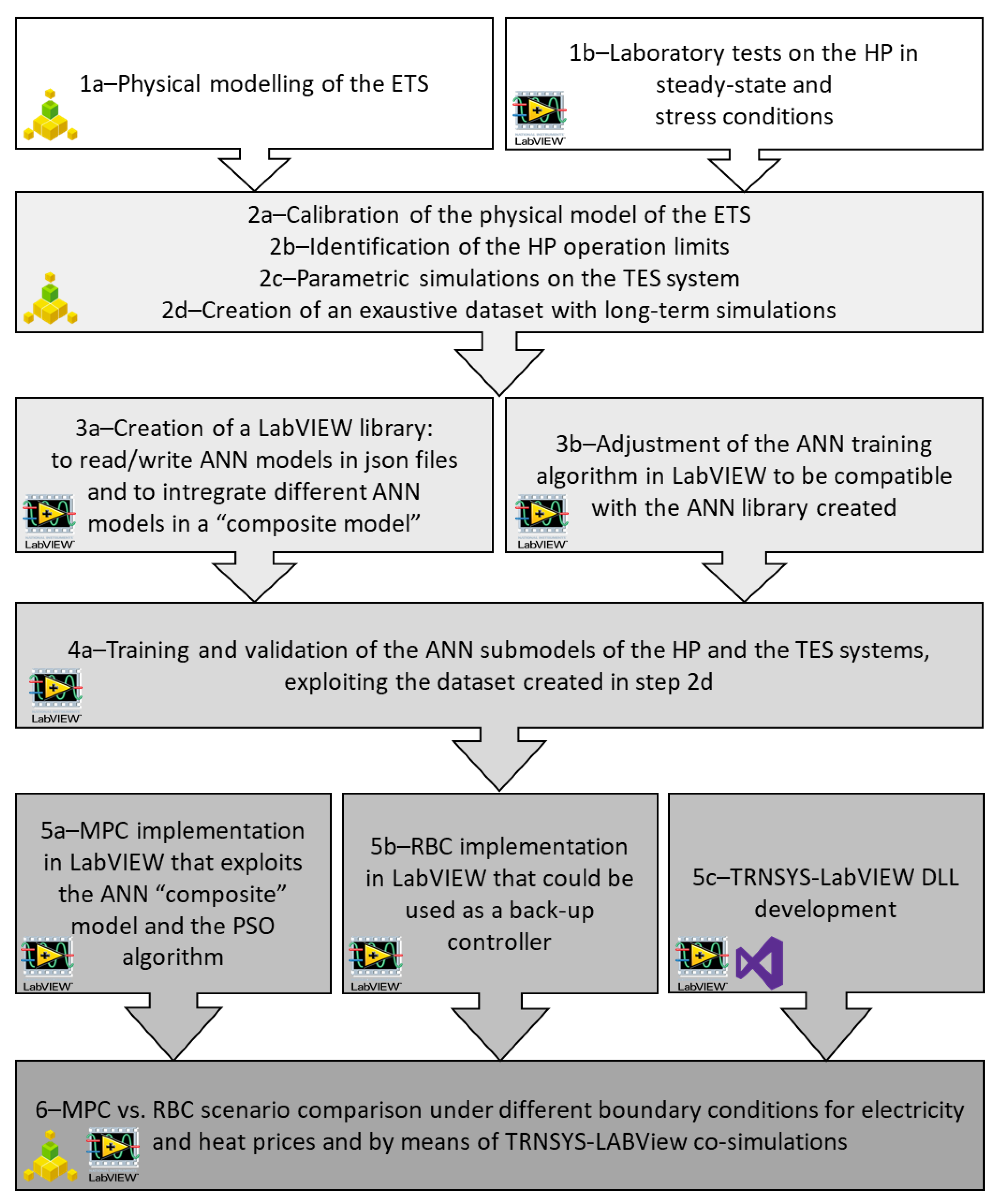
2. Materials and Methods

To investigate a smart power-to-heat operation considering the implementation of a demand response (DR) strategy and exploiting the local heat pump and thermal energy storage system at the ETS level, a simulation tool for the application of model predictive control (MPC) has been developed. It is based on algorithms that belong to the field of artificial intelligence (AI) and uses a reduced order model (ROM) to make predictions of the substation performance. The following six sections offer a description of the methodology applied to develop and test the MPC according to the six steps of the flowchart in Figure 2.

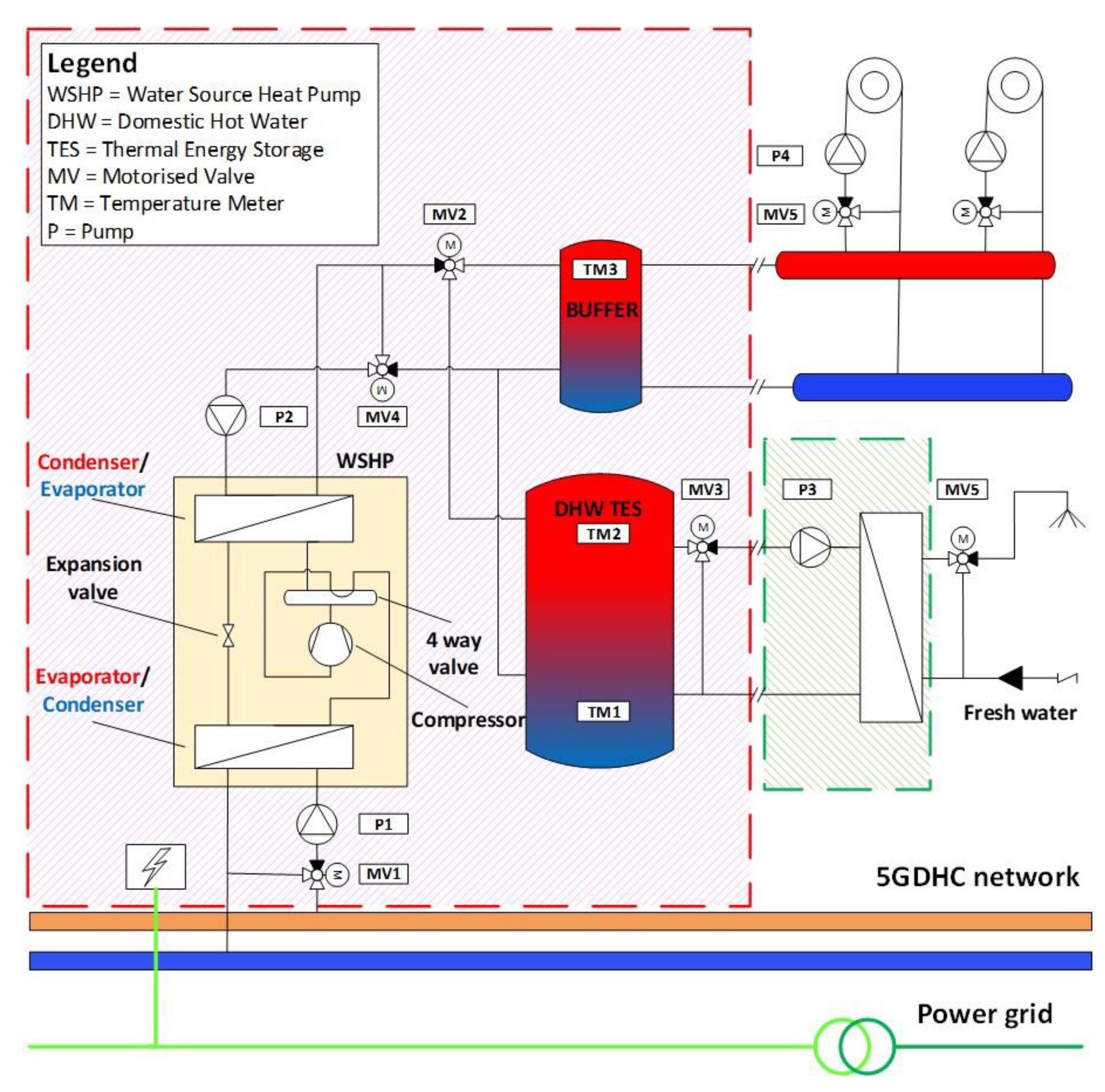
2.1. Physical Modelling and Laboratory Test of the 5GDHC Energy Transfer Station (ETS)

The 5GDHC ETS physical model developed has the equivalent capacity of one of the two single-compressor speed WSHPs available at the Energy Exchange Laboratory of EURAC Research [51] that has been used for model calibration and validation. The ETS, modelled in TRNSYS, consists of a number of components that are connected according to the layout reported in Figure 3 with some improvements with respect to the standard installation of heat pump systems. In fact, the mixing valves at the DHW recirculation circuit (MV3) has been added to limit the maximum supply temperature of the DHW recirculation circuit of 50 °C, so that the thermal losses could be minimised if the ETS is operated for excess-charging the DHW. Moreover, the mixing valves MV4 at the WSHP condenser has been considered to control the inlet temperature at 45 °C during the DHW mode (30 °C during SH mode), limiting the destratification process that occurs at each turn-on of the WSHP. The latter is a single-stage unit with a capacity of 23 kWh connected to an insulated buffer for space heating (SH) or space cooling (SC), with a capacity of 0.375 m³ that satisfies the common requirement of heat pump manufacturers to have a buffer capacity of about 15 ÷ 20 L/kWh of the heat pump. Moreover, a DHW TES system is needed to cover the peaks in the DHW demand, and its size has been determined following the parametric analysis presented in the next section. The ETS satisfies the energy demands of a small multi-family house with five floors and two apartments per floor located in Rome. The specific DHW demand has been estimated at 24 kWh/m² per year, and it has been created by generating the draw-off profile with the software DHWcalc V.2.02b [27] with a time step of one minute, considering an occupancy level of 2 people/apartment and the specific hot water demand of 40/l (person/day). The time step used in the simulation is one minute to achieve a high resolution and a realistic temperature profile inside the thermal energy storage tanks by satisfying the maximum volume change ratio in one time step for each node of the modelled tank. The TRNSYS types used are type 927 of the TESS library to model the WSHP using a performance map validated with laboratory tests, as described in the next section; type 110 to model the variable speed hydraulic pumps and type 534 of the TESS library to model the DHW TES and the space heating/cooling buffer; and type 11f, type 11h, and custom type 843 to model both diversion valves and mixing points. The 5GDHC network itself has not been modelled, and it has been considered as an ideal heat source that always supplies the ETS at a constant temperature of 15 °C. The investigation of the 5GDHC network, as well as the optimal sizing of the 5GDHC ETS, is out of the scope of this work.

The other activity carried out in parallel with modelling consists of laboratory tests under steady-state and stress conditions at the Energy Exchange Lab. The steady-state tests were performed with nominal constant flow rates, operating the WSHP both at a constant inlet temperature at the evaporator and varying the inlet temperature at the condenser and vice versa. In particular, the inlet temperature at the condenser was varied with steps of 5 °C between 30 °C and 55 °C, whereas the inlet temperature at the evaporator was varied with steps of 2.5 °C between 10 °C and 20 °C. Stress tests were carried out to identify the real operation limits of the WSHP to avoid that the compressor stops its operation due to some alarms that would require a manual reset. In fact, some of these could arise if the advanced controller operates the WSHP in a different way compared to the standard operation by excess charging the thermal energy storage at a very high temperature. In the next section, it will be presented how the laboratory test results were used in this study to validate the ETS model.

2.2. Physical Model Calibration, WSHP Limits, and Parametric Simulations on the Thermal Energy Storage System

The key performance indicators (KPIs) used for model calibration and validation have been suggested by ASHRAE Guideline 14 [52] and adopted in general for building energy simulations, like in Harmer and Henze (2015) [53] and in Ruiz et al. (2017) [54]. Considering ${\zeta }_j$, the jth output variable of the system under study, $w_{{\zeta }_j}$ a weight associated with the jth output variable, $n$ samples of a generic output variable ${\zeta }_j$ and $m_i$ the measured values of the variable ${\zeta }_j,$ and $s_i$ the simulated values of the variable ${\zeta }_j$ (obtained from a system model providing the same measured inputs), the KPIs considered are the normalised mean bias error for the variable ${\zeta }_j$ ($NMB{E}_{{\zeta }_j}$), the coefficient of variation of the root mean square error for the variable ${\zeta }_j$ ($CVRMS{E}_{{\zeta }_j}$), the goodness of fit of the $\mathrm{NMBE}$ for different variables ${\zeta }_j$ ($GO{F}_{NMBE}$), and the goodness of fit of the $\mathrm{CVRMSE}$ for different variables ${\zeta }_j$ ($GO{F}_{CVRMSE}$), according to the Equations (1)–(4). The total goodness of fit ($GO{F}_{Tot}$) in Equation (5) was obtained considering the weights $w_{NMBE}=w_{CVRME}=1$.

$$NMB{E}_{{\zeta }_j}=\frac{1}{{\overline{m}}_j} \frac{{\sum }_{i=1}^n\left(m_{j,i}-s_{j,i}\right)}{n} \cdot 100(\%)$$

(1)

$$CVRMS{E}_{{\zeta }_j}= \frac{1}{{\overline{m}}_j} \sqrt{\frac{{\sum }_{i=1}^n{\left(m_{j,i}-s_{j,i}\right)}^2}{n-1}}\cdot 100(\%)$$

(2)

$$GO{F}_{NMBE}=\sqrt{\frac{{\sum }_{j=1}^J\left(w_{{\zeta }_j}{}^2\cdot NMB{E}_{{\zeta }_j}{}^2\right)}{{\sum }_{j=1}^J\left(w_{{\zeta }_j}{}^2\right)}}$$

(3)

$$GO{F}_{CVRMSE}=\sqrt{\frac{{\sum }_{j=1}^J\left(w_{{\zeta }_j}{}^2\cdot CVRMS{E}_{{\zeta }_j}{}^2\right)}{{\sum }_{j=1}^J\left(w_{{\zeta }_j}{}^2\right)}}$$

(4)

$$\begin{array}{c}GO{F}_{Tot}=\sqrt{\frac{w_{NMBE}{}^2\cdot {\left(GO{F}_{NMBE}\right)}^2+w_{CVRMSE}{}^2\cdot {\left(GO{F}_{CVRMSE}\right)}^2}{w_{NMBE}{}^2+w_{CVRMSE}{}^2}}\\ =\frac{\sqrt{2}}{2}\cdot \sqrt{GO{F}_{NMBE}{}^2+GO{F}_{CVRMSE}{}^2}\end{array}$$

(5)

In this study, the WSHP has been modelled by means of a performance map in the form of a look-up table using type 927 of the TRNSYS TESS library. This model, after reading the inlet temperatures and flow rates as inputs, provides as outputs the outlet temperatures and electrical and thermal energy flows at the evaporator and condenser side of the WSHP, which are the results of linear interpolation in a specified range. The performance map adopted was derived from previous laboratory tests on a similar WSHP with the same refrigerant R410A [55], and the linear interpolation coefficients were reassessed. Moreover, the performance map was normalised with respect to the WSHP capacity so that it can be used for machines with different sizes. These normalisation parameters are the rated heating capacity (${\dot{Q}}_{HP,h}^{*}$) and the rated electricity capacity in the heating mode ($P_{el,HP,h}^{*}$), which the calibrated values were found with an exhaustive parametric search using half of the lab dataset.

The results of the calibration are reported in Figure 4; on the left, with the NMBE vs. CVRMSE plot for the different outputs of the WSHP model and, on the right, with the $GO{F}_{NMBE} \mathrm{vs}. GO{F}_{RMSE}$ plot, calculated according to the equations presented above. The circled point in Figure 4b is the one with the lowest values of the $GO{F}_{Tot}$ equal to 2.6%, which corresponds to ${\dot{Q}}_{HP,h}^{*}=22.98 k{W}_{th}$ and $P_{el,HP,h}^{*}=4.08 k{W}_{el}$. The rest of the dataset was used for validation purposes, whose results are shown in Figure 5, where the outputs of the calibrated WSHP model are plotted and compared with the measured quantities. In Figure 5a, the agreement of the outlet temperatures at the evaporator ($T_{out,source}$) and at the condenser ($T_{out,load}$) during the two tests in the heating mode is shown, assuming a constant inlet temperature at the evaporator ($T_{in,source}$) and constant inlet temperature at the condenser ($T_{in,load}$), respectively. In Figure 5b, the corresponding thermal power at the evaporator ($Q_{source}$) and condenser ($Q_{load}$), as well as the electricity consumption ($P_{el}$), are shown. It can be noticed that the simulated profiles fall within the measurement uncertainty band (in grey) in almost all operating conditions. The fluctuations of the measured thermal power quantities are because of the effects of the control system during the laboratory tests.

Beyond the steady-state tests, additional stress tests were performed to identify the real operation limits of the WSHP in the heating mode using water in all the circuits. For this reason, starting from four extreme operating points (A, B, C, and D) of the standard operation map in the heating mode (referred to as ΔT = 5 °C on both the evaporator and condenser side, as reported by the manufacturer) shown in Figure 6a, these tests were performed to achieve different temperature differences on both the evaporator and the condenser side. This was possible by varying the volumetric flowrates within the ranges achievable at the lab: a minimum of 1.8 m³/h and a maximum of 3.5 m³/h at the evaporator and a minimum of 2.2 m³/h and a maximum of 4 m³/h at the condenser. In particular, the operating condition of points A and B could represent the ones of a WSHP supplied by a low-temperature source, like groundwater, respectively, in SH and DHW modes. Similarly, points D and C represent the operation of a WSHP supplied by a high-temperature source. The main results of the stress tests can be summarised as follows:

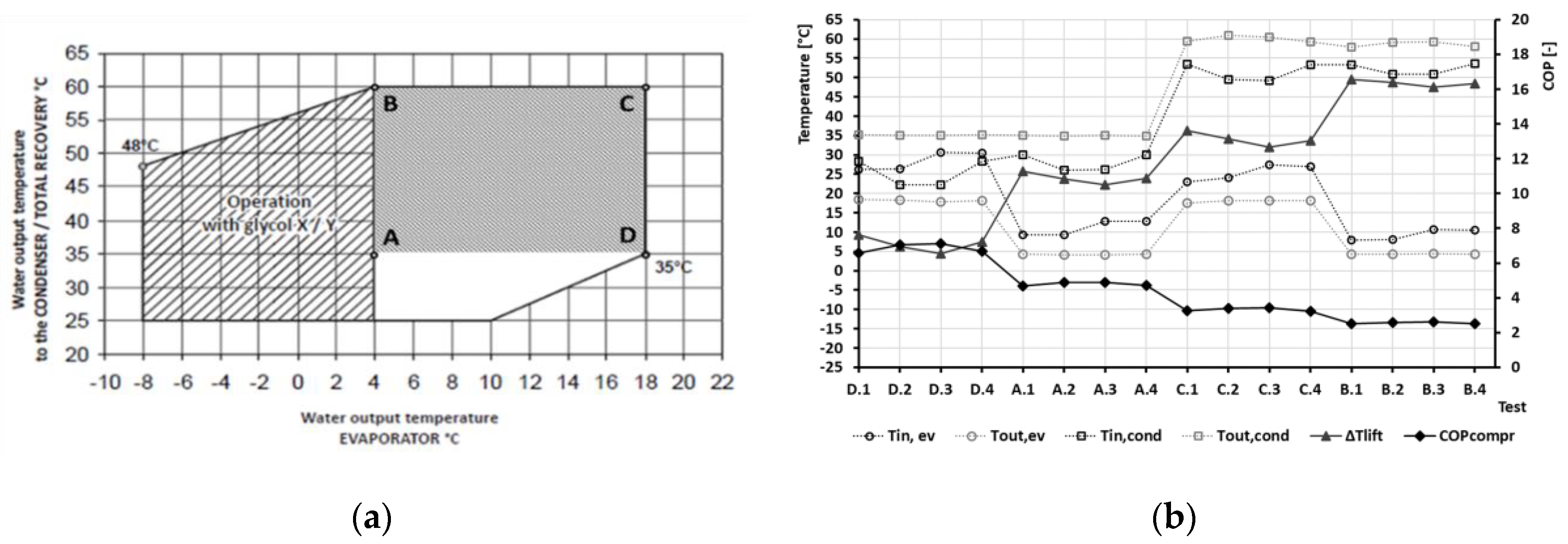
• The outlet temperature at the evaporator ($T_{out,eva}$) must be higher than 4.9 °C to avoid a freezing alarm. This critical condition can be reached during the WSHP operation around points A and B of Figure 6a.
• The outlet temperature at the condenser ($T_{out,cond}$) must be lower than 57.3 °C to avoid an alarms for refrigerant high temperature (max 118 °C) and high pressure (max 40 bar at the compressor outlet). This critical condition can be reached during the WSHP operation around points B and C of Figure 6a.

The coefficient of performance (COP) variation, together with the average temperature values for the different operating steady-state conditions, are shown in Figure 6b. Four operating conditions were explored around each extreme operation point (A, B, C, and D). As expected, the smaller the difference between the average temperatures at the evaporator and at the condenser (ΔT_lift), the higher is the COP. Nevertheless, it is important to highlight that, at some operating points (D2, D3, and D4), the WSHP can operate with an inlet temperature at the evaporator that is higher than the inlet temperature at the condenser. Among the tests at each single extreme operation point (e.g., A1, A2, A3, and A4), a slight increase in the COP can be observed for tests in which the difference between the inlet and outlet temperature at the condenser is maximised.

Finally, a parametric analysis has been performed on the 5GDHC ETS model to define the optimal size of the thermal energy storage system to meet the DHW load satisfying the user’s comfort and to assess the optimal height of the temperature sensor used to control the DHW TES. This was done to verify the impact of thermal energy storage capacity exploitation by the MPC controller, together with the operational limitations of the WSHP, such as the maximum outlet temperature at the condenser, as mentioned above. The analysis was performed considering a control based on a hysteresis rule that has a fixed lower bound of 45 °C and a variable dead-band that has been varied. The overall values of the parameters that have been varied one at a time are:

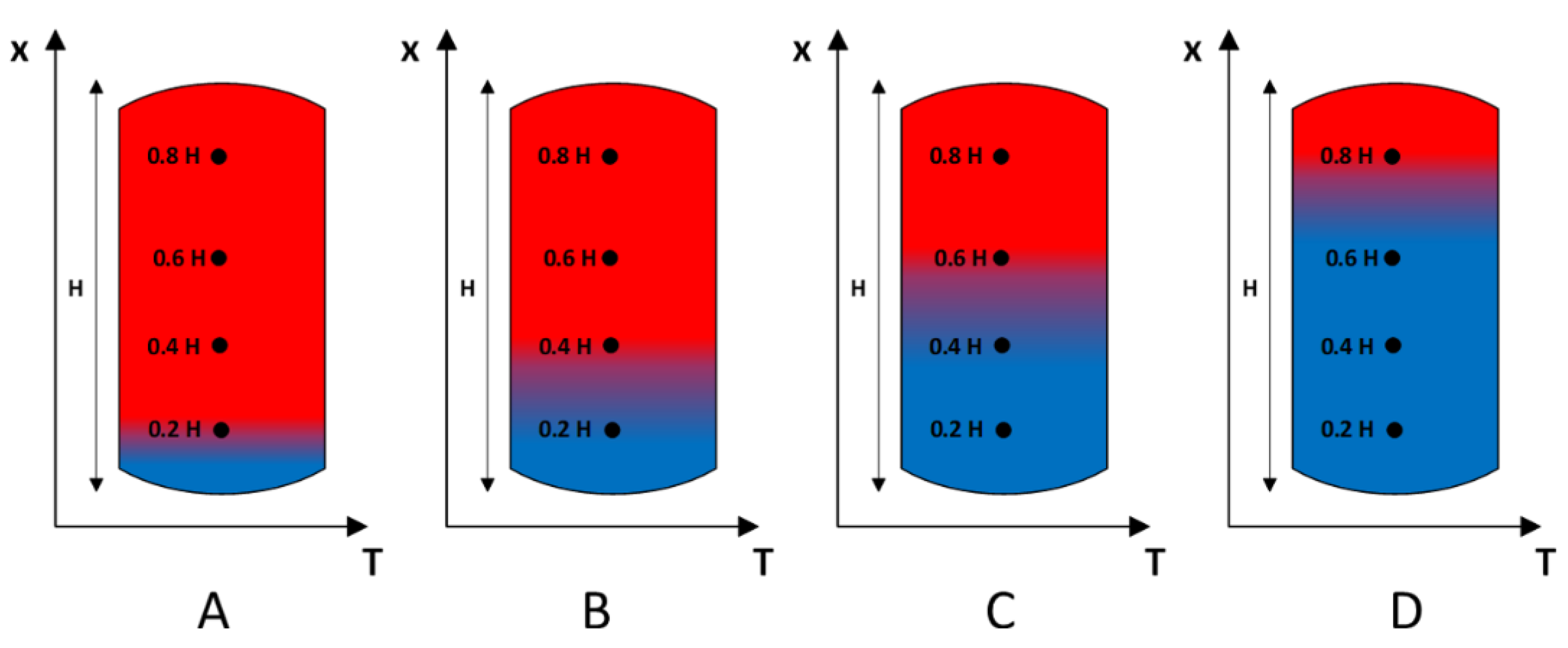
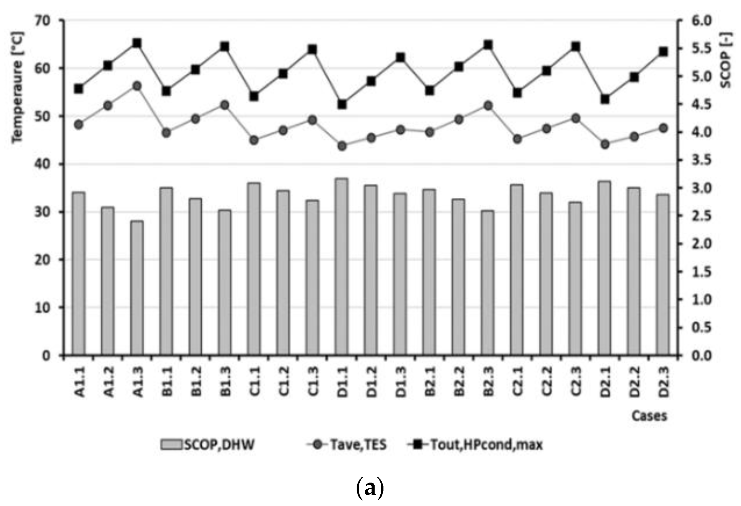
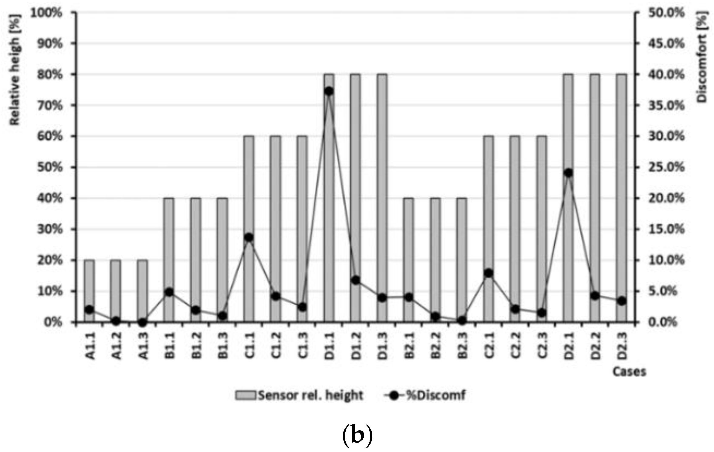
• four values for the relative height of the sensor used to control the thermal energy storage temperature, as shown in Figure 7, and identified with a letter (A = 20%, B = 40%, C = 60%, and D = 80%);
• two values for the DHW TES volume identified by a number that follows the letter, equal to 0.5 m³ (1) and 1 m³ (2), respectively; and
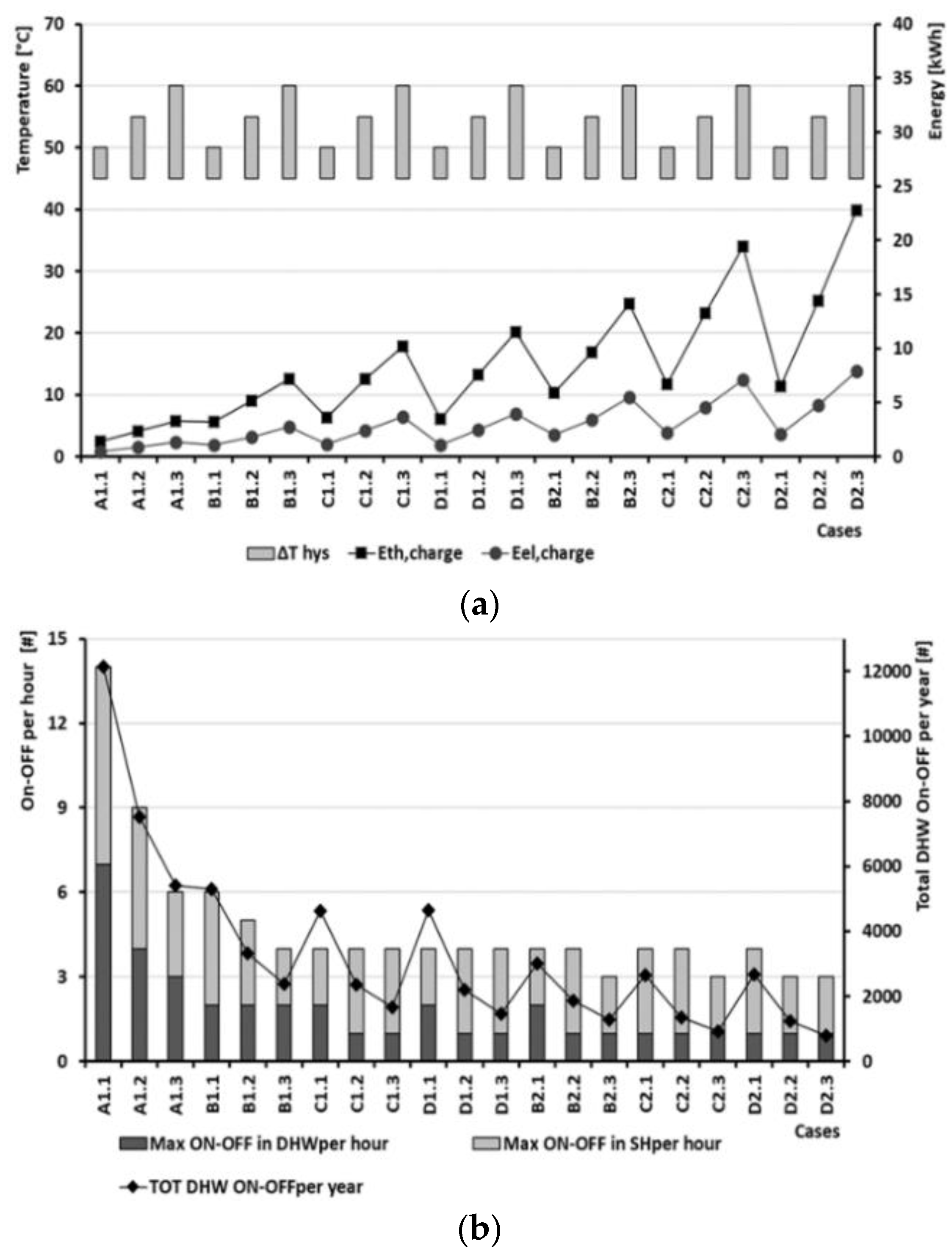
• three values for the dead-band of the hysteresis implemented in the rule-based control that was fixed equal to 5 °C (1), 10 °C (2), and 15 °C (3).

For instance, case C2.2 represents the case where the sensor position has been fixed at the 60% (C) of the thermal energy storage total height, the thermal energy storage has a volume of 1 m³ (2), and the hysteresis band is equal to 10 °C (2), so that, during a charging process, the temperature of the sensor is increased from 45 °C to 55 °C. This is the final solution adopted for the development of the reduced order model (ROM) of the substation as a conclusion of the results presented in Section 3.1 obtained by assessing the following KPIs:

• ${\%}_{discomfort}$ that aims at evaluating the fraction of time when the DHW tap water has a temperature below 44 °C with respect to the total draw-off period, according to Equation (6). It allows verifying whether the boundary conditions concerning the thermal energy storage capacity and control settings satisfy the user’s comfort.
• ${\overline{E}}_{th,charge}$ and ${\overline{E}}_{el,charge}$, which are the average thermal energy supplied by the WSHP to the DHW TES and average electricity consumption per single charge, calculated as the yearly energy quantity divided by the yearly number of on-off cycles, according to Equations (7) and (8), respectively.

  $${\%}_{discomfort}=\frac{DHW draw off duration with T_{out,DHW}<44 °\mathrm{C} \left[h\right]}{Total DHW draw off duration with\left[h\right]} [\%]$$

  (6)

  $${\overline{E}}_{th,charge}=\frac{E_{th,hp,DHW,tot}}{N_{ON-OFF,tot}} \left[KWh\right]$$

  (7)

  $${\overline{E}}_{el,charge}=\frac{E_{el,hp,DHW,tot}}{N_{ON-OFF,tot}} \left[KWh\right]$$

  (8)

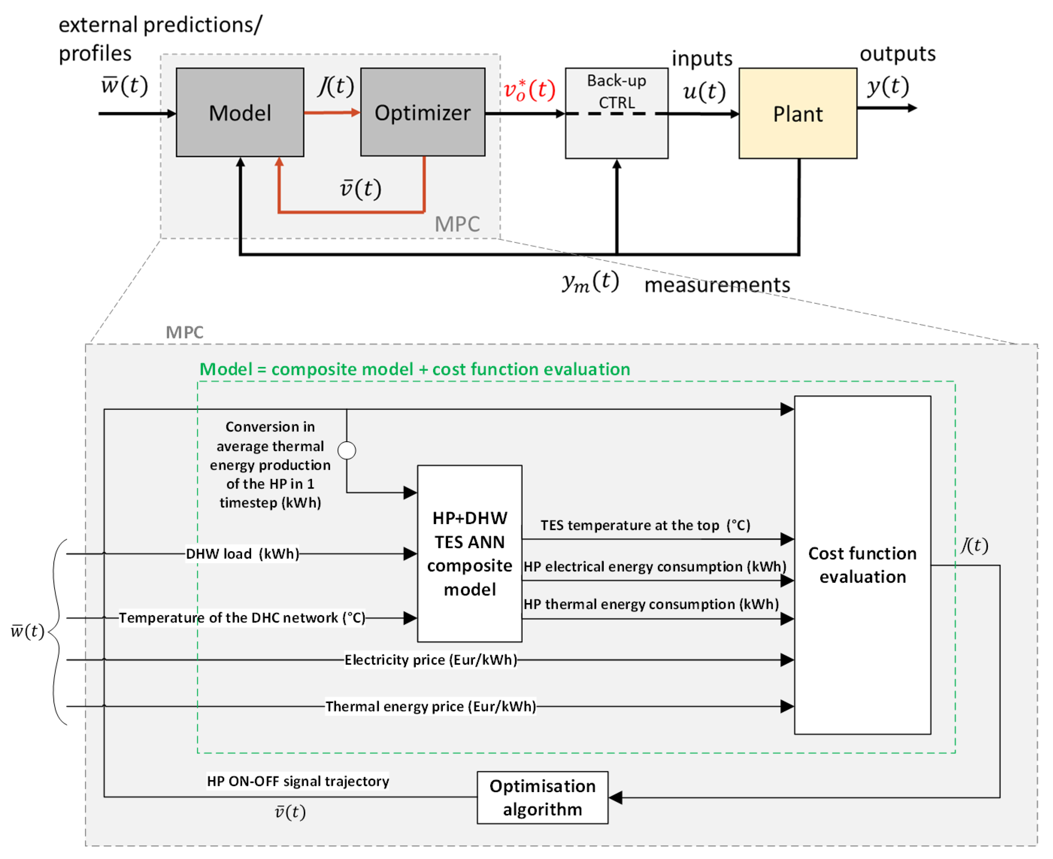
2.3. ANN Model and Training Algorithm

In this work, the advanced controller were implemented in LabVIEW in the form of artificial neural network-based model predictive control (ANN-MPC). A literature review of this application for HVAC systems can be found in Afram et al. (2017) [56]. Here, ANNs were used for a prediction problem by creating a reduced order model (ROM) of the 5GDHC ETS for smart charging of the DHW TES system. The benefits of such kinds of ROMs include the fact that the data-driven approach allows for building simplified models, even with the same architecture, that can be connected in a bottom-up approach neglecting some less-important variables. Moreover, using real-time data of the system, the ANN can be retrained periodically, unlocking the “adaptative” potential of such kinds of control solutions and reducing the deviations between the boundary and operation conditions and the one considered in the design phase. This reduces the effects of the mismatch between the design model and the current operation of the system on the controller performance.

However, such models need a large amount of training data and a tool for raw data collection and preprocessing together with a training algorithm to periodically update the model. Compared to white-box physical models, ANNs are a form of black-box models that exhibit the advantage of low computational effort when running simulations. This can be very useful for running MPC algorithms in embedded systems; however, the results must be interpreted carefully, because they cannot be explained easily.

The ROM of the 5GDHC ETS was built in a modular fashion using the same ANN architecture to model each component: one for the WSHP and one for the DHW TES. This ANN architecture is based on a nonlinear autoregressive network with exogenous inputs (NARX), also called “dynamic” or “recurrent” ANNs, because they have a feedback loop that provide “memory” capabilities typical of dynamic systems; here, a tapped delay line (TDL) of one time step is used so that the model outputs at time t depend not only on the inputs at time t but, also, on the model inputs and outputs at the previous time step t − 1. The network structure includes one hidden layer with 15 neurons, as well as the tangent-sigmoid and the linear activation functions in the hidden and output layers, respectively. Due to the good performance observed, reported in the next section, an optimisation of the ANN features has not been performed in this work. The variables considered as inputs and outputs of the ANN models are:

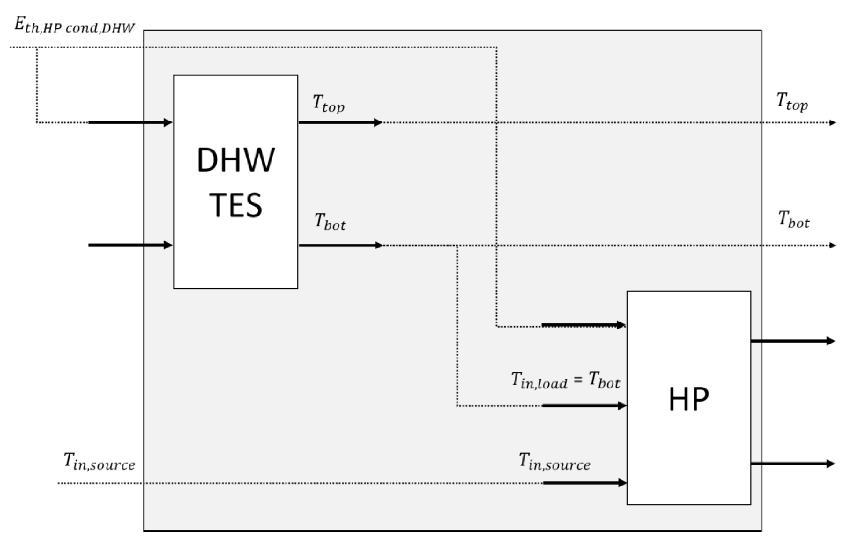
• $E_{th,HP cond,DHW}$ is the thermal energy delivered by the on-off WSHP to the DHW TES in one control time step (4 kWh_th) and represents the control input $u_0^{*}$ provided according to the results of the MPC algorithms during the on-line simulation (see Section 2.5).
• $E_{th,sub,DHW load}$ is the forecasted DHW load to cover under the hypothesis of the perfect prediction.
• $T_{top}$ and $T_{bot}$ are the temperatures at the top and at the bottom of the TES, respectively.
• $T_{in,load}$ is the inlet temperature at the WSHP condenser here equal to $T_{bot}$.
• $T_{in,source}$ is the inlet temperature at the WSHP evaporator.
• $E_{el,sub, DHW}$ is the electricity consumption of the substation during the DHW operation as a sum of the consumption of the heat pump compressor ($E_{el,HP,DHW}$) and the hydraulic pumps ($E_{el,aux,DHW}$).
• $E_{th,HP eva,DHW}$ is the thermal energy extracted by the WSHP from the DHC network.

The composite ROM model was obtained by properly connecting the inputs and outputs of the two ANNs, according to Figure 8. $E_{th,HP cond,DHW}$ and $E_{th,sub,DHW load}$ are the two inputs of the DHW TES ANN model that provides as outputs $T_{top}$ and $T_{bot},$ whereas, for the heat pump ANN model $E_{th,HP cond,DHW}$, $T_{bot}$ and $T_{in,source}$ are the inputs and $E_{el,SUB, DHW}$, $E_{th,HP eva,DHW}$ are the outputs. The ambient temperature of the room was not used as the input, since it is not commonly monitored in the mechanical room where the ETS are installed; here, it has been assumed constant and equal to 15 °C. The recurrent ANN models were implemented in LabVIEW, creating a dedicated object-oriented class for regression or prediction problems. The training algorithm adopted is a heuristic modification of the traditional backpropagation algorithm that includes a variable learning rate α that is adjusted during the course of the training. Network training is performed in an open-loop mode; i.e., since during the training, the target values are available, there is no need to feed back to the ANN input the estimation of the output, instead providing accurate inputs to the model directly from the training dataset.

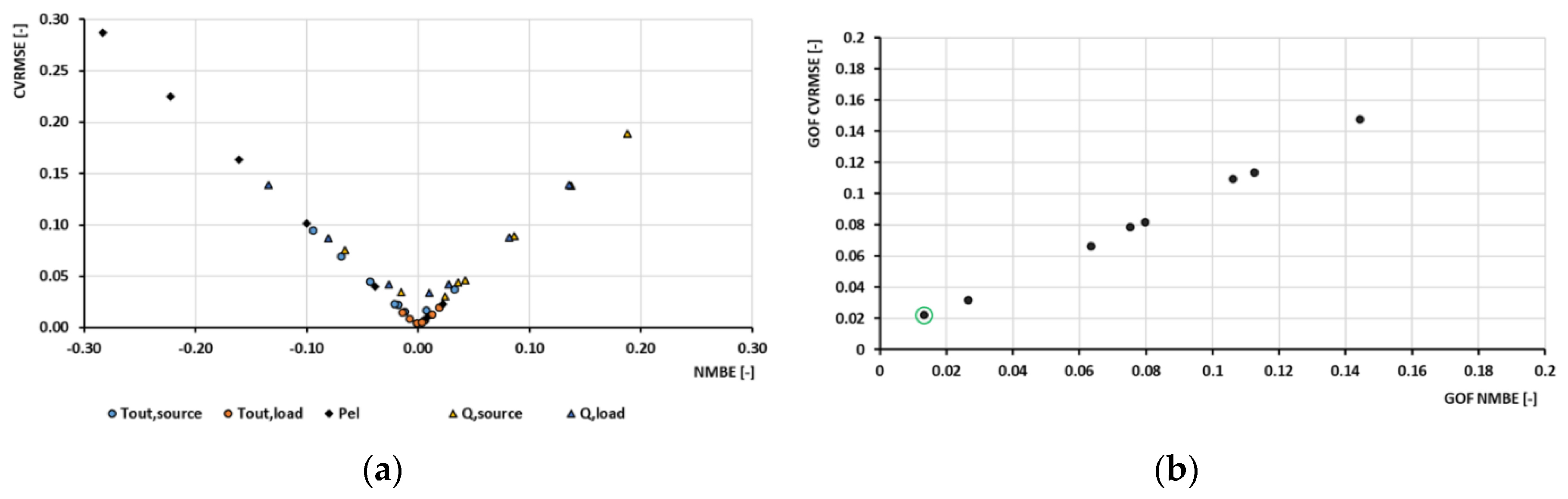
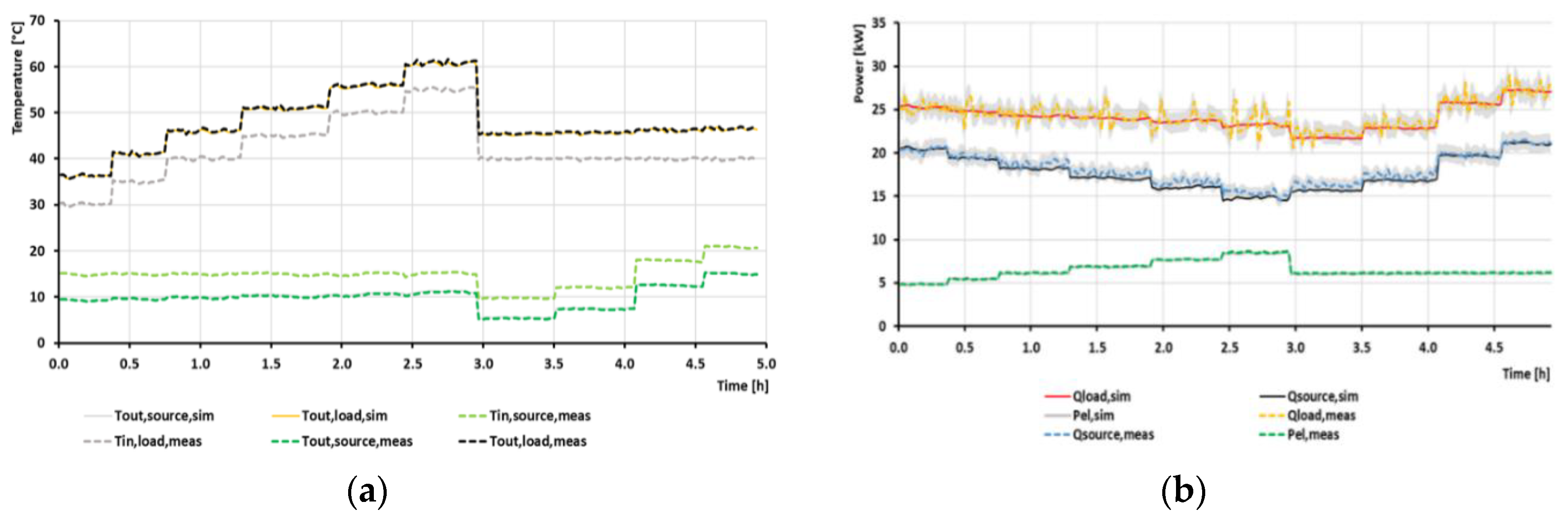
2.4. ANN Model Training and Validation Results

The two ANN models of the WSHP and DHW TES system were trained by using the results of 20 days of numerical simulations from the TRNSYS calibrated model. The dataset time resolution is 10 min, which is the same as the control time step at which the MPC solves the optimisation problem and provides the on-off signal. This choice has been adopted according to the information reported in Curtis and Pine (2012) [57], who claim that it is important to avoid short cycling conditions for heat pumps by setting a minimum off-time between 6 and 10 min and a minimum runtime of 10 min. The first is useful so that, after a prior run, the refrigerant pressures in the heat pump are re-equalised, avoiding a restart of the compressor under high-pressure and high-temperature conditions. The second allows maintaining an adequate level of lubrication of the compressor that is compromised if there are short runtime periods, because the oil is transported out of the compressor by the refrigerant and could be trapped in the refrigerant circuit, leading to potential damage at the following starts.

The training dataset from the numerical simulations was created using a rule-based controller (RBC) for the DHW operation, trying to allow the ANN models to explore a wide range of operation conditions. Both the implementations of the RBC and MPC controller are explained in the next section. Creating such a large training dataset was not done with laboratory tests, because it would be very expensive. The performance of the ANNs models was assessed by evaluating the KPIs listed in Equations (1)–(5) for the ANN outputs vs. the target values by using a validation dataset of 24 h (144 time steps of 10 min) that has not been used for training purposes and are shown in Figure 9. Different from the training phase, the model validation is performed in a closed loop fashion of the NARX process feeding back to the ANN inputs errors in the estimated outputs at the previous time step t-1. The KPI results listed in

Table 1. Closed-loop results of the domestic hot water thermal energy storage (DHW TES) and water-source heat pump artificial neural network (WSHP ANN) model validations. NMBE: normalised mean bias error, CVRMSE: coefficient of variation of the root mean square error, GOF: goodness of fit, T_top and T_bot: temperature at the top and bottom, and HP: heat and power.

DHW TES ANN Model			WSHP ANN Model
$NMBE T_{top}$	$NMBE T_{bot}$		$$\begin{gathered} NMBE \\ {E}_{el,SUB, DHW} \end{gathered}$$	$$\begin{gathered} NMBE \\ {E}_{th,HP eva,DHW} \end{gathered}$$
(%)	(%)		(%)	(%)
0.065%	0.117%		0.164%	−0.735%
$CVRMSE T_{top}$	$CVRMSE T_{bot}$		$$\begin{gathered} CVRMSE \\ {E}_{el,SUB, DHW} \end{gathered}$$	$$\begin{gathered} CVRMSE \\ {E}_{th,HP eva,DHW} \end{gathered}$$
(%)	(%)		(%)	(%)
3.4%	4.6%		1.3%	0.8%
$GO{F}_{MBE}$	$GO{F}_{RMSE}$	$GO{F}_{Tot}$	$GO{F}_{MBE}$	$GO{F}_{RMSE}$	$GO{F}_{Tot}$
(%)	(%)	(%)	(%)	(%)	(%)
0.1%	4.0%	2.9%	0.53%	1.08%	0.85%

show that a high accuracy is obtained in the prediction of the WSHP electricity consumption ($E_{el,SUB, DHW}$) and thermal energy extracted from the DHC network at the evaporator ($E_{th,HP eva,DHW}$). The ANN model for the DHW TES results in a somewhat lower accuracy with respect to the WSHP model; nevertheless, the NRMSE for both of the two outputs, the temperature at the top ($T_{top}$) and at the bottom ($T_{bot}$), are below 5% over a simulation time of 24 h.

2.5. MPC Implementation with an RBC Back-Up Controller and TRNSYS-LabVIEW Dynamic Link Library (DLL)

Model predictive control (MPC) is an emerging control technology that has been used since the 1980s in the chemical process industry. Nowadays, its implementation with HVAC systems is mainly devoted to large commercial and institutional buildings that employ building energy management (BEM) systems, as shown in the literature review of Afram and Janabi-Sharifi (2014) [58]. Other MPC implementations of heat pumps and chiller-based systems coupled with thermal energy storage are presented in Kajgaard et al. (2013) [59], Henze et al. (2004) [46], and Yudong Ma et al. (2009) [60]. Moreover, MPC has been studied in the context of a low-temperature district heating network in Vivian et al. (2017) [61] and in Knudsen and Petersen (2017) [62].

MPC employs a model of the process whose identification is usually demanding in terms of effort depending on the complexity of the process or the model fidelity to achieve. By performing real-time simulations, this model is employed to make a prediction of the future outputs of the process according to a sequence of future inputs that one would like to apply. In this study, MPC is implemented according to the block diagram of Figure 10 to solve a constrained optimisation problem in real-time at each control time step (10 min)—hence, to find the best sequence of control actions ${\overline{v}}^{*}\left(t\right)$ that minimises (or maximises) a given performance index over a time window. Only the first element $v_0^{*}\left(t\right)$ is applied to the plant at the current time step $t$, discarding the rest of the control action sequence. In this study, the so-called receding horizon control approach is applied, consisting of a shift of the time window forward at each control time step where, once the new measurements have been acquired and the state of the model is updated, the optimisation problem is solved again. Moreover, a blocking technique is applied in a way that the control horizon (M) is shorter than the prediction horizon (N) to reduce the effort in solving the optimisation problem. For this work, the prediction horizon is equal to 180 min (N = 18 time steps), and the control horizon is equal to 60 min (M = 6 time steps); since the length of the control action sequence vector ${\overline{v}}^{*}\left(t\right)$ is less than the number of time steps in the prediction horizon (M < N), the last value of ${\overline{v}}^{*}\left(t\right)$ is maintained constant for the rest of the simulation.

MPC can be employed both as a low-level (slave) or high-level (master/supervisory) controller. When MPC is operated in a supervisory fashion, it is a common practice to implement it with the objective being to minimise the operating costs of the system. For this reason, this kind of solution as adopted here is usually referred to as economic model predictive control (EMPC). Due to the nonlinearities of the ANNs, a different solution from traditional hard-computing MPC implementation was applied to solve the optimisation problem. In fact, in this study, the binary form of the particle swarm optimisation (PSO) algorithm proposed by Kennedy and Eberhart (1997) [63] is used, as it is suitable for this kind of application of solving multi-objective optimisation problems with low computational times [56]. Moreover, a similar use was performed in Amarasinghe et al. (2015) [64] and in other HVAC applications, as reviewed in Afram et al. (2017) [56]. PSO is a metaheuristic algorithm that belongs to the field of swarm intelligence, biologically inspired by the collective behaviour of species like birds (flocking) and fishes (shoaling and schooling). The algorithm, derived from the “perturbed PSO” [65] available in the Advanced Metaheuristics Algorithms library implemented by Derouiche M. L. (2015) and available at [66], is implemented in such a way that a population of interacting agents directly search for the minimum of the cost function $J\left(t\right)$ in a multidimensional domain with no information about its gradient (unknown environment).

As mentioned above, the MPC application presented in the following covers a power-to-heat operating strategy controlling the WSHP of the 5GDHC ETS. The constrained optimisation problem aims at minimising the operating costs of the ETS over the prediction horizon with N time steps ($t_0,\dots ,t_k,\dots , t_{k+N-1}$). For this reason, the terms reported in the cost function $J\left(t_j\right)$ in Equation (9) considers the electricity consumption of the substation $E_{el,SUB,DHW}\left(t_j\right)$, the specific cost of electricity $c_{el}\left(t_j\right)$, the thermal energy supplied by the 5GDHC network to the substation $E_{th,HP eva,DHW}\left(t_j\right),$ and its specific cost $c_{th,dhc} \left(t_j\right)$. The last term of the objective function considers a “state $s\left(t_j\right)$ change cost” to minimise the on-off switching events of the heat pump that are a cause of inefficiencies, as well as electrical and mechanical stresses, of its components. The problem constraints consider having the minimum temperature at the top of the DHW TES higher than 45 °C to satisfy the user´s comfort (Equation (10)) and the maximum temperature at the top of the DHW TES lower than 55 °C to satisfy the operating limits of the WSHP, as shown from the stress tests results above (Equation (11)).

$$J\left(t_j\right)={\displaystyle \sum _{j=k}^{k+N-1}}{c}_{el}\left(t_j\right)E_{el,SUB,DHW}\left(t_j\right)+{\displaystyle \sum _{j=k}^{k+N-1}}{c}_{th,dhc} E_{th,HP eva,DHW}\left(t_j\right)+\beta {\displaystyle \sum _{j=k}^{k+N-1}}\left|s\left(t_j\right)-s\left(t_{j-1}\right)\right|$$

(9)

$$\underset{t_j\ge 0}{min}{T}_{top}\left(t_j\right)>T_{top,,min}=45 °\mathrm{C}$$

(10)

$$\underset{t_j\ge 0}{max}{T}_{top}\left(t_j\right)<T_{top,max}=55 °\mathrm{C}$$

(11)

Referring to the block diagram in Figure 10 (bottom), the MPC implementation consists of a matrix of variables $\overline{w}\left(t\right)$ that are computed externally, like the DHW load perfect prediction, prediction of the DHC network supply temperature, and profiles of the electricity and thermal energy prices over the prediction horizon. The output of the optimisation algorithm $\overline{w}\left(t\right)$ is a binary vector that considers the different trajectories of the WSHP on-off state and allows directly evaluating the “state-change cost”. Nevertheless, to be compatible with the input required in the ANN model implementation, the on signal is expressed as the average thermal energy that the WSHP is able to provide to DHW TES in one control time step of 10 min, equal to 4 kWh_th. Finally, since the bound constraints of Equations (10) and (11) have been implemented by applying the external static penalty technique, as in [67], and adding this to the rest of the cost function $J\left(t_j\right)$, the top temperature of the DHW TES system, together with the electricity and thermal energy consumption, are all forecasted by the ANN model and are considered in the cost function evaluation section.

As shown in the block diagram of Figure 10 (top), a back-up controller is used to filter the MPC signal $v_0^{*}\left(t\right)$. It consists of an RBC that includes two levels of hysteresis: one operating in parallel to the MPC, such that, if the top temperature of the DHW TES drops below 45 °C, it is charged up to 50 °C, and another hysteresis operating in series with the MPC so that, if the top temperature of the DHW TES exceeds 55 °C, the WSHP is disabled (bypassing the MPC on signal) and can be turned on only if it is below 53 °C. This has been adopted to make the overall controller more robust with respect to the soft-constrains implementation. Finally, there was the need to create a bidirectional communication between the MPC controller implemented in LabVIEW and the physical model in TRNSYS that has been used as the plant to test the controller. For this reason, a dedicated TRNSYS type has been programmed in C++ that gets inputs and provides outputs at each simulation time step to the MPC algorithm by means of a dynamic link library (DLL) programmed in LabVIEW.

2.6. MPC vs. RBC Scenario Boundary Conditions

To assess the MPC performance, a simulation test was performed for a period of 31 days (January 2017) coupling TRNSYS and LabVIEW by means of the DLL presented above. The study aimed at comparing a standard rule-based control (RBC) strategy applied to the ETS with the model predictive control (MPC) one presented above for the DHW TES management when a price variation of the electricity tariff was introduced. This was done according to a time-of-use demand response strategy based on the Italian tariff D1. Accordingly, the on-peak hours were defined as the period between 8:00 and 19:00 on workdays, while the rest were considered off-peak hours. The RBC operated by means of a hysteresis that was active when the DHW TES top temperature dropped below 45 °C and stopped the charging process when it reached 50 °C. Conversely, the MPC controller was capable of exploiting its prediction capabilities to optimise the ETS operation.

The guiding principle of the analysis is based on the following considerations introduced also in a previous publication [68]. Charging the thermal energy storage beyond the currently needed value introduces a drawback: the higher the temperature, the larger are both the drop of the WSHP coefficient of performance $\left(COP\right)$ and additional thermal losses ($E_{th,add. losses})$. For the sake of simplicity, by accounting only for the electricity cost as an optimisation parameter ($c_{el}$ is in EUR/kWh), the thermal energy needed $(E_{th}) \mathrm{would} \cos \mathrm{t} c_{el,peak}{E}_{th}/{\mathrm{COP}}_{max}$ during the peak hour when it is produced at the minimum storage temperature, while it would cost $c_{el,off-peak}(E_{th}+E_{th,add. losses})/\mathrm{COP}$ when produced in advance at a higher temperature. To achieve savings in the electricity bill, the inequality of Equation (12) must hold. Rearranging it to Equation (13), it can be observed that there is a lower limit of the COP for the thermal energy storage excess charge process that depends on the electricity price ratio between off-peak hours and on-peak hours and the ratio between the additional thermal losses introduced with respect to the thermal energy produced ($E_{th}$). Charging the DHW TES at higher temperatures is worthwhile only if the electricity costs ratio compensates at least the additional thermal losses introduced. Moreover, for 5GDHC ETS, the variation of the COP affects the weight of the electricity bill with respect to the bill for the thermal energy drawn off from the DHC grid, because the higher the COP, the higher the amount of thermal energy extracted by the WSHP at the evaporator.

$$\frac{c_{el,off-peak}(E_{th}+E_{th,add. losses})}{COP}<\frac{c_{el,peak}{E}_{th}}{CO{P}_{max}}$$

(12)

$$COP>\left(\frac{c_{el,off-peak} }{c_{el,peak}}\right) \left(1+ \frac{E_{th,add. losses}}{E_{th}}\right) CO{P}_{max}$$

(13)

The time-of-use demand response scenario analysis performed in this study is simplified to verify the effects reported above during the MPC (scenarios 1 and 2) with respect to a standard RBC (baseline) operation for charging the DHW TES. The conditions set have in common the same ETS plant and DHW load, while the economic boundary conditions are the following:

• The price of the thermal energy extracted from the 5GDHC grid is considered constant and equal to 0.05 (EUR/kWh) for the different scenarios.
• The electricity tariff during off-peak hours is considered constant and equal to 0.15 (EUR/kWh) for the different scenarios.
• The electricity tariff during on-peak hours varies, and it is equal to 0.30 (EUR/kWh) for MPC scenario 1 and 0.60 (EUR/kWh) for MPC scenario 2.

3. Results and Discussion

The results of this study have been divided into two parts: in Section 3.1, the parametric analysis on the DHW TES system introduced in Section 2.2 is discussed, whereas, in Section 3.2, the performance of the system operated with an advanced control strategy is compared with respect to a rule-based one under different boundary conditions, as presented in Section 2.6.

3.1. Parametric Analysis on the DHW TES System

The cases analysed reported on the x-axis of Figure 11 and Figure 12 consider four values of the relative height of the sensor, with the two extremes that are A at 20% (bottom) and D at 80% (top) of the tank height; two values of the DHW TES size 0.5 m³ (1) and 1 m³ (2); and three values of the dead-band of the hysteresis at 5 °C (1), 10 °C (2), and 15 °C (3). The results presented in Figure 11a show the average thermal energy storage temperature ($T_{ave,TES}$) and the maximum WSHP condenser outlet temperature ($T_{out,HPcond,max}$) for the different cases. It can be observed that, for a given thermal energy storage volume, a higher height of the temperature sensor and a larger hysteresis band have the same effects in terms of a lower $T_{ave,TES},$ as well as $T_{out,HPcond,max},$ achieving a higher $SCO{P}_{DHW}$ for the DHW operation. The variation of the thermal energy storage volume has almost no effect on these variables.

In Figure 11b, the sensor height is compared with the discomfort percentage for the different cases. The results show that, for given values of the hysteresis band and thermal energy storage volume, the higher the position of the sensor, the larger is the ${\%}_{discomfort},$ because it results in a smaller hot volume of the thermal energy storage to absorb a peak in the DHW demand. For instance, in case D1.1, where a thermal energy storage of 0.5 m³ is controlled with a hysteresis of 5 °C using the sensor at the top ($H_{rel}$ of 80%), for 37.3% of the draw off time, the tap water temperature is lower than 44 °C. This issue can be resolved in two ways: either by increasing the thermal energy storage volume or by increasing the hysteresis band, where the latter appears to have a larger positive effect on ${\%}_{discomfort}$ reduction with respect to the increase of the thermal energy storage volume.

The results shown in Figure 12a are referring to the average thermal energy supplied by the WSHP to the DHW TES (${\overline{E}}_{th,charge}$) and average electricity consumption per single charge (${\overline{E}}_{el,charge}$). Both increase by varying the hysteresis band or the thermal energy storage volume. Assessing the ${\overline{E}}_{el,charge}$ is useful to understand the amount of electricity that can be consumed during a DHW charging process if the WSHP is operated as an equivalent electrical battery to provide load flexibility and resilience to the electricity grid.

Finally, the maximum hourly number of on-off switching events, reported in Figure 12b, is calculated in order to verify when it exceeds values suggested by the literature, identified as between 3 and 4 [57], to limit the low efficiency and component failure. In this context, case A1.1 is the worst, with a maximum number of hourly switching cycles equal to 14 due to both SH and DHW operation starts and the highest number of yearly switching events in the DHW mode. This is a consequence of the fact that the sensor used to control the DHW TES is located at the bottom ($H_{rel}$ of 20%) close to the pipe connection of the return pipeline of the DHW recirculation system. When a large DHW draw-off occurs in the apartments, the temperature in the return pipe of the DHW can be very low (~20 °C), causing an instantaneous turn-on of the WSHP in the DHW mode, even if the thermal energy storage is fully charged. For this reason, the installation of the temperature sensor at the bottom of the DHW TES must be avoided.

The best compromise to satisfy the different constraints described above is obtained for case C2.2, which assumes a DHW TES capacity of 1 m³, a temperature sensor position at a height $H_{rel}$ of 60%, and a maximum range in controlling the thermal energy storage temperature between 45 °C and 55 °C. Under these conditions, alarms for the high temperature/pressure of the refrigerant are avoided, the ${\%}_{discomfort}$ assessed is 2.2%, and a decent amount of energy can be stored in the DHW TES during a full charge $\left({\overline{E}}_{th,charge}=13.2 kW{h}_{th} \mathrm{and}{\overline{E}}_{el,charge}=4.6 kW{h}_{el}\right)$. This configuration of the DHW TES is used for the rest of the study.

3.2. Results of the Rule-Based Control (RBC) vs. Model Predictive Control (MPC) Scenario Analysis

The second part of the results section aims at comparing the MPC to RBC performance under the boundary conditions of the time-of-use demand response scenario presented in Section 2.6, where the electricity tariff variation occurs twice per day and only during weekdays, whereas the price of the thermal energy extracted from the DHC network is constant. The selected ETS configuration is the one of C2.2 (see Section 3.1), and the MPC operates to minimise the energy bill and “state change” of the WSHP according to the cost function of Equation (9). The prediction horizon has been set equal to 180 min (N = 18 time steps) and the control horizon equal to 60 min (M = 6 time steps). The results of this analysis are reported in

Table 2. Energy assessment of the scenario analysis. RBC: rule-based controller and MPC: model predictive control.

Scenario	cEel,off-peak EUR/kWh)	cEel,peak (EUR/kWh)	Ttop,max (°C)	Tave (°C)	Eel,SUB,DHW (kWh)	Eth,HP eva,DHW (kWh)	COPsub (-)	Eel,SUB,DHW,off-pek (kWh)	Eel, SUB,DHW,peak (kWh)	Non (-)
Baseline (RBC)			50.4	40.7	439.6	993.1	2.78	258	182	101
MPC scenario 1	0.15	0.3	54.3	41.3	454.3	1025.2	2.70	290	165	159
			7.7%	1.5%	3.3%	3.2%	−3.0%	12.4%	−9.5%	57.4%
MPC scenario 2	0.15	0.6	54.3	41.4	458.2	1033.6	2.68	302	156	169
			7.8%	1.9%	4.2%	4.1%	−3.7%	17.3%	−14.2%	67.3%

and

Table 3. Economic assessment of the scenario analysis. C_Eel,tot: total cost for the electrical energy, C_Eth,tot: total cost for the thermal energy and UEB_tot: total utility energy bill.

Scenario	cEel,off-peak (EUR/kWh)	cEel,peak (EUR/kWh)	cEth,dhc (EUR/kWh)	CEel,tot (EUR)	CEth,tot (EUR)	UEBtot (EUR)
Baseline (RBC)	0.15	0.3	0.05	93.2	49.7	142.9
MPC scenario 1	0.15	0.3	0.05	92.8	51.3	144.1
Rel. var.				−0.4%	3.2%	0.8%
Baseline (RBC)	0.15	0.6	0.05	147.9	49.7	197.5
MPC scenario 2	0.15	0.6	0.05	139.0	51.7	190.7
Rel. var.				−6.0%	4.1%	−3.5%

, whereas the relative differences between MPC scenarios 1 and 2 with respect to the baseline (RBC operation) are shown in Figure 13. It can be observed that, for MPC scenarios 1 and 2, the advanced controller operates by charging the DHW TES more frequently with respect to the baseline scenario. In fact, the number of start-up signals ($N_{ON}$) of the heat pump in the DHW mode increases by about 57.4%, and 67.3%, respectively. Thus, it results, on average, in less thermal energy being provided by the heat pump to the DHW TES during a single charge with respect to the standard charging process of the baseline scenario. From the energy assessment reported in Table 2, on the one hand, it emerges that extending the ΔT range operation between 45 and 55 °C for extra charging of the DHW TES with the MPC controller results in a higher maximum temperature at the top ($T_{top,max}$) and average temperature ($T_{ave}$) of the DHW TES. This, in turn, affects the performance of the WSHP, with a drop in the coefficient of performance ($CO{P}_{sub}$) by about 3–4% for both MPC scenarios. As a consequence, both the electricity and thermal energy consumptions of the ETS coming from the electrical and thermal grids ($E_{el,SUB,DHW}$ and $E_{th,HP eva,DHW}$) increase. On the other hand, focusing on the electricity uses of the substation, it emerges that the larger the electricity tariff variation between off-peak and peak hours, the larger is the electricity load shifted from peak to off-peak hours. The reduction in the electricity consumption during peak hours ($E_{el,SUB,DHW,peak}$) is about 10% for MPC scenario 1 and about 14% for MPC scenario 2, where a larger electricity tariff variation occurs. Nonetheless, the reduction of electricity consumption during peak hours is at the expense of an increase in consumption during off-peak hours ($E_{el,SUB,DHW,off-peak}$) that is larger, because, during the MPC scenarios, the ETS operates at a lower $CO{P}_{sub}$.

From the economic assessment reported in Table 3, one infers that there are no savings on the total utility energy bill ($UE{B}_{tot}$) in MPC scenario 1, while small savings are achieved in MPC scenario 2, since the savings obtained by the limited time-of-use price variation in MPC scenario 1 do not compensate for the additional energy consumptions due to the drop in the $CO{P}_{sub}$ and additional thermal losses of the TES. In MPC scenario 2, it can be noticed that the situation is different. The on-peak electricity tariff is four times that of the off-peak hours. The $UE{B}_{tot}$ has a reduction of 3.5% with respect to the baseline, which makes the MPC control slightly attractive with respect to a standard RBC control operation in terms of electricity costs, in addition to the load shift effect.

4. Conclusions

This work presents a detailed assessment on 5GDHC energy transfer station (ETS) operations, offering solutions for improving the management of the local domestic hot water (DHW) thermal energy storage (TES) system. The first implementation and test of an ANN-based model predictive controller (MPC) are discussed. This tool aims at unlocking the smart control of the 5GDHC ETS to cover the DHW load by exploiting the thermal capacity of the DHW TES. In this context, one of the main outcomes of the work is that a modular ANN approach can be a valuable solution for implementing an adaptive reduced order model of the ETS that could be periodically retrained with monitoring data, reducing the mismatch between the design and real control conditions.

Furthermore, a test presented in this study deals with the energetic and economic performance assessments of the 5GDHC ETS, comparing its operation under a model predictive control (MPC) strategy with respect to a standard rule-based control (RBC). Different scenarios were analysed considering different electricity prices, and the results show that excess charging of the thermal energy storage leads to a drop in system performance due to a lower COP and higher thermal energy losses that are not always compensated economically by the savings achieved due to smart-charging the thermal energy storage during off-peak hours. In fact, the MPC is able to offer economic savings of about 3.5% (over a period of one month) on the total utility energy bill only when the electricity price during on-peak hours is four times the value at off-peak hours. However, it is important to point out that these results were obtained under specific boundary conditions where the electricity tariff variation occurs twice per day and only during weekdays and under the assumption of a perfect prediction of the DHW load.

Further research is needed to evaluate the performance under real-time pricing (RTP) and other demand response programs, larger prediction horizons, the extension of the smart control to a pool of substations, and assess the optimal architecture of the ANN models. It is important to highlight that, in this study, the MPC operation contributes to shaving the electricity peak-load up to 14% by shifting demand to off-peak hours with a constant supply temperature of the 5GDHC network. However, conversely from air-source heat pump system applications, the supply temperature of a 5GDHC system can be considered an additional variable that can be manipulated by the DHC operator to further gain elasticity in pooling 5GDHC substations to participate in demand response programs. This kind of energy flexibility and resilience provided by advanced control are additional benefits that will become increasingly important under high-penetration scenarios of distributed renewable energy resources where 5GDHC systems could cooperate with power grids in decentralised smart energy systems.

References

1. European Commission. An EU Strategy on Heating and Cooling; European Commission: Brussels, Belgium, 2016. [Google Scholar]
2. Ruiz, I.B.; Wecker, K. Where is Europe’s Air Safe to Breathe? Available online: https://www.dw.com/en/where-is-europes-air-safe-to-breathe/a-46189571 (accessed on 14 February 2020).
3. Kranzl, L.; Hartner, M.; Müller, A.; Resch, G.; Fritz, S.; Fleiter, T.; Herbst, A.; Rehfeldt, M.; Manz, P.; Zubaryeva, A.; et al. Heating & Cooling Outlook Until 2050, EU-28; Hotmaps Project; European Commission: Brussels, Belgium, 2018. [Google Scholar]
4. Persson, U.; Werner, S. Quantifying the Heating and Cooling Demand in Europe; European Commission: Brussels, Belgium, 2015. [Google Scholar]
5. Wheatcroft, E.; Wynn, H.; Lygnerud, K.; Bonvicini, G.; Leonte, D. The Role of Low Temperature Waste Heat Recovery in Achieving 2050 Goals: A Policy Positioning Paper. Energies 2020, 13, 2107. [Google Scholar] [CrossRef] [Green Version]
6. DHC+ Technology Platform. District Heating & Cooling: A Vision Towards 2020-2030-2050; Euroheat & Power: Brussels, Belgium, 2012. [Google Scholar]
7. Prando, D.; Prada, A.; Ochs, F.; Gasparella, A.; Baratieri, M. Analysis of the energy and economic impact of cost-optimal buildings refurbishment on district heating systems. Sci. Technol. Built Environ. 2015, 21, 876–891. [Google Scholar] [CrossRef]
8. European Commission. The European Green Deal Investment Plan and Just Transition Mechanism Explained. Available online: https://ec.europa.eu/commission/presscorner/detail/en/qanda_20_24 (accessed on 14 February 2020).
9. Lund, H.; Østergaard, P.A.; Chang, M.; Werner, S.; Svendsen, S.; Sorknæs, P.; Thorsen, J.E.; Hvelplund, F.; Mortensen, B.O.G.; Mathiesen, B.V.; et al. The status of 4th generation district heating: Research and results. Energy 2018, 164, 147–159. [Google Scholar] [CrossRef]
10. Fallahi, Z.; Henze, G.P. Interactive Buildings: A Review. Sustainability 2019, 11, 3988. [Google Scholar]
11. EU H2020 FLEXYNETS Project. Available online: www.flexynets.eu (accessed on 10 January 2020).
12. EU Interreg D2Grids Project. Available online: http://www.nweurope.eu/projects/project-search/d2grids-increasing-the-share-of-renewable-energy-by-accelerating-the-roll-out-of-demand-driven-smart-grids-delivering-low-temperature-heating-and-cooling-to-nwe-cities/ (accessed on 10 July 2020).
13. EU Life4HeatRecovery Project. Available online: http://www.life4heatrecovery.eu (accessed on 15 June 2020).
14. EU H2020 REWARDHeat Project. Available online: https://www.rewardheat.eu (accessed on 15 June 2020).
15. EU H2020 ReUseHeat Project. Available online: https://www.reuseheat.eu (accessed on 15 June 2020).
16. EU H2020 TEMPO Project. Available online: https://www.tempo-dhc.eu (accessed on 15 June 2020).
17. EU H2020 WEDISTRICT Project. Available online: https://www.wedistrict.eu (accessed on 15 June 2020).
18. EU H2020 RELaTED Project. Available online: http://www.relatedproject.eu (accessed on 15 June 2020).
19. H2020 Upgrade DH Project. Available online: http://www.upgrade-dh.eu (accessed on 15 June 2020).
20. EU H2020 COOL DH Project. Available online: http://www.cooldh.eu (accessed on 15 June 2020).
21. EU H2020 KeepWarm Project. Available online: https://keepwarmeurope.eu (accessed on 15 June 2020).
22. EU H2020 THERMOS Project. Available online: https://www.thermos-project.eu (accessed on 15 June 2020).
23. EU Interreg HeatNet NWE Project. Available online: http://www.nweurope.eu/projects/project-search/heatnet-transition-strategies-for-delivering-low-carbon-district-heat/ (accessed on 15 June 2020).
24. EU Interreg ENTRAIN Project. Available online: https://www.interreg-central.eu/Content.Node/ENTRAIN.html (accessed on 15 June 2020).
25. Ruesch, F.; Haller, M. Potential and limitations of using low-temperature district heating and cooling networks for direct cooling of buildings. In Proceedings of the International Conference CISBAT 2017 Future Buildings & Districts—Energy Efficiency from Nano to Urban Scale, Lausanne, Switzerland, 6–8 September 2017; Volume 122, pp. 1099–1104. [Google Scholar]
26. Vetterli, N.; Sulzer, N.; Menti, U.P. Energy monitoring of a low temperature heating and cooling district network. Energy Procedia 2017, 122, 62–67. [Google Scholar]
27. Bünning, F.; Wetter, M.; Fuchs, M.; Müller, D. Bidirectional low temperature district energy systems with agent-based control: Performance comparison and operation optimization. Appl. Energy 2018, 209, 502–515. [Google Scholar] [CrossRef] [Green Version]
28. Ruesch, F.; Rommel, M.; Scherer, J. Pumping power prediction in low temperature district heating networks. In Proceedings of the International Conference CISBAT 2015 Future Buildings and Districts Sustainability from Nano to Urban Scale, Lausanne, Switzerland, 9–11 September 2015; LESO-PB, EPFL. pp. 753–758. [Google Scholar]
29. Vetterli, N.; Sulzer, M. Dynamic analysis of the low-temperature district network “Suurstoffi” through monitoring. In Proceedings of the International Conference CISBAT 2015 Future Buildings and Districts Sustainability from Nano to Urban Scale, Lausanne, Switzerland, 9–11 September 2015; LESO-PB, EPFL. pp. 517–522. [Google Scholar]
30. Prasanna, A.; Dorer, V.; Vetterli, N. Optimisation of a district energy system with a low temperature network. Energy 2017, 137, 632–648. [Google Scholar] [CrossRef]
31. Ruesch, F.; Scherer, J.; Kolb, M. Erdreich als Speicher—Grosse Anergienetze. In Proceedings of the Internationale Konferenz zur Simulation gebäudetechnischer Energiesysteme, Winterthur, Switzerland, 8–9 September 2016. [Google Scholar]
32. Gautschi, T. Energiekonzept Anergienetz Hönggerberg; ETH Zürich, Infrastrukturbereich Immobilien: Zürich, Switzerland, 2015. [Google Scholar]
33. La Boucle d’eau Tempérée à Énergie Géothermique; AFPG—Association Française des Professionnels de la Géothermie: Paris, France, 2019.
34. Revesz, A.; Jones, P.; Dunham, C.; Davies, G.; Marques, C.; Matabuena, R.; Scott, J.; Maidment, G. Developing novel 5th generation district energy networks. Energy 2020, 201, 117389. [Google Scholar] [CrossRef]
35. Long, N.L. Reduced Order Models for Rapid Analysis of Ambient Loops for Commercial Buildings. Ph.D. Thesis, University of Colorado, Boulder, CO, USA, 2018. [Google Scholar]
36. Buffa, S.; Cozzini, M.; D’Antoni, M.; Baratieri, M.; Fedrizzi, R. 5th generation district heating and cooling systems: A review of existing cases in Europe. Renew. Sustain. Energy Rev. 2019, 104, 504–522. [Google Scholar]
37. Boesten, S.; Ivens, W.; Dekker, S.C.; Eijdems, H. 5th generation district heating and cooling systems as a solution for renewable urban thermal energy supply. Adv. Geosci. 2019, 49, 129–136. [Google Scholar]
38. Von Rhein, J.; Henze, G.P.; Long, N.; Fu, Y. Development of a topology analysis tool for fifth-generation district heating and cooling networks. Energy Convers. Manag. 2019, 196, 705–716. [Google Scholar] [CrossRef]
39. National Renewable Energy Laboratory (NREL) URBANopt Advanced Analytics Platform. Available online: https://www.nrel.gov/buildings/urbanopt.html (accessed on 1 March 2020).
40. Modelica Buildings Library. Available online: https://simulationresearch.lbl.gov/modelica/ (accessed on 3 March 2020).
41. Sommer, T.; Sulzer, M.; Wetter, M.; Sotnikov, A.; Mennel, S.; Stettler, C. The reservoir network: A new network topology for district heating and cooling. Energy 2020, 199, 117418. [Google Scholar] [CrossRef]
42. Abugabbara, M.; Javed, S.; Bagge, H.; Johansson, D. Bibliographic analysis of the recent advancements in modeling and co-simulating the fifth-generation district heating and cooling systems. Energy Build. 2020, 110260. [Google Scholar] [CrossRef]
43. Wirtz, M.; Kivilip, L.; Remmen, P.; Müller, D. 5th Generation District Heating: A novel design approach based on mathematical optimization. Appl. Energy 2020, 260, 114158. [Google Scholar] [CrossRef]
44. Wirtz, M.; Kivilip, L.; Remmen, P.; Müller, D. Quantifying Demand Balancing in Bidirectional Low Temperature Networks. Energy Build. 2020, 224, 110245. [Google Scholar] [CrossRef]
45. Miara, M.; Günther, D.; Leitner, Z.L.; Wapler, J. Simulation of an Air-to-Water Heat Pump System to Evaluate the Impact of Demand-Side-Management Measures on Efficiency and Load-Shifting Potential. Energy Technol. 2014, 2, 90–99. [Google Scholar] [CrossRef]
46. Henze, G.P.; Felsmann, C.; Knabe, G. Evaluation of optimal control for active and passive building thermal storage. Int. J. Therm. Sci. 2004, 43, 173–183. [Google Scholar] [CrossRef]
47. Pau, M.; Cunsolo, F.; Vivian, J.; Ponci, F.; Monti, A. Optimal Scheduling of Electric Heat Pumps combined with Thermal Storage for Power Peak Shaving. In Proceedings of the 2018 IEEE International Conference on Environment and Electrical Engineering and 2018 IEEE Industrial and Commercial Power Systems Europe (EEEIC/I&CPS Europe), Palermo, Italy, 12–15 June 2018. [Google Scholar]
48. Rastegarpour, S.; Gros, S.; Ferrarini, L. MPC approaches for modulating air-to-water heat pumps in radiant-floor buildings. Control Eng. Pract. 2020, 95, 104209. [Google Scholar] [CrossRef]
49. Beghi, A.; Cecchinato, L.; Cosi, G.; Rampazzo, M. A PSO-based algorithm for optimal multiple chiller systems operation. Appl. Therm. Eng. 2012, 32, 31–40. [Google Scholar] [CrossRef]
50. D’Ettorre, F.; Conti, P.; Schito, E.; Testi, D. Model predictive control of a hybrid heat pump system and impact of the prediction horizon on cost-saving potential and optimal storage capacity. Appl. Therm. Eng. 2019, 148, 524–535. [Google Scholar] [CrossRef]
51. Eurac Research Energy Exchange Lab. Available online: http://www.eurac.edu/en/research/technologies/renewableenergy/Infrastructure/Pages/Energy-Exchange-Lab.aspx (accessed on 15 December 2017).
52. ASHRAE 14-2002. In Guideline 14-2002: Measurement of Energy and Demand Savings; American Society of Heating, Refrigeration and Air-Conditioning Engineers: Atlanta, GA, USA, 2002.
53. Harmer, L.C.; Henze, G.P. Using calibrated energy models for building commissioning and load prediction. Energy Build. 2015, 92, 204–215. [Google Scholar] [CrossRef]
54. Ruiz, G.; Bandera, C. Validation of Calibrated Energy Models: Common Errors. Energies 2017, 10, 1587. [Google Scholar] [CrossRef] [Green Version]
55. Menegon, D.; Fedrizzi, R. FP7 INSPIRE Project D4.7: Report on Laboratory Dynamic Tests. 2016. Available online: https://cordis.europa.eu/project/id/314461/reporting (accessed on 21 August 2020).
56. Afram, A.; Janabi-Sharifi, F.; Fung, A.S.; Raahemifar, K. Artificial neural network (ANN) based model predictive control (MPC) and optimization of HVAC systems: A state of the art review and case study of a residential HVAC system. Energy Build. 2017, 141, 96–113. [Google Scholar] [CrossRef]
57. Curtis, R.; Pine, T. Effects of Cycling on Domestic GSHPs. Supporting Analysis to EA Technology Simulation/Modelling; Mimer Geoenergy: Cornwall, UK, 2012. [Google Scholar]
58. Afram, A.; Janabi-Sharifi, F. Theory and applications of HVAC control systems—A review of model predictive control (MPC). Build. Environ. 2014, 72, 343–355. [Google Scholar] [CrossRef]
59. Kajgaard, M.U.; Mogensen, J.; Wittendorff, A.; Veress, A.T.; Biegel, B. Model predictive control of domestic heat pump. In Proceedings of the American Control Conference (ACC), Washington, DC, USA, 17–19 June 2013. [Google Scholar]
60. Ma, Y.; Borrelli, F.; Hencey, B.; Packard, A.; Bortoff, S. Model predictive control of thermal energy storage in building cooling systems. In Proceedings of the 48h IEEE Conference on Decision and Control (CDC) Held Jointly with 2009 28th Chinese Control Conference, Shanghai, China, 15–18 December 2009; pp. 392–397. [Google Scholar]
61. Vivian, J.; Jobard, X.; Hassine, I.B.; Pietrushka, D.; Hurink, J.L. Smart Control of a District Heating Network with High Share of Low Temperature Waste Heat. In Proceedings of the 12th Conference on Sustainable Development of Energy, Water and Environmental Systems-SDEWES, Dubrovnik, Croatia, 4–8 October 2017. [Google Scholar]
62. Knudsen, M.D.; Petersen, S. Model predictive control for demand response of domestic hot water preparation in ultra-low temperature district heating systems. Energy Build. 2017, 146, 55–64. [Google Scholar] [CrossRef]
63. Kennedy, J.; Eberhart, R.C. A Discrete Binary Version of the Particle Swarm Algorithm; IEEE: Orlando, FL, USA, 1997. [Google Scholar]
64. Amarasinghe, K.; Wijayasekara, D.; Carey, H.; Manic, M.; He, D.; Chen, W. Artificial neural networks based thermal energy storage control for buildings. In Proceedings of the IECON 2015—41st Annual Conference of the IEEE Industrial Electronics Society, Yokohama, Japan, 9–12 November 2015; pp. 005421–005426. [Google Scholar]
65. Zhao, X. A perturbed particle swarm algorithm for numerical optimization. Appl. Soft Comput. 2010, 10, 119–124. [Google Scholar]
66. Advanced Metaheuristics Algorithms by ENIT. Available online: http://sine.ni.com/nips/cds/view/p/lang/it/nid/216789 (accessed on 25 October 2018).
67. Derouiche, M.L.; Bouallègue, S.; Haggège, J.; Sandou, G. LabVIEW Perturbed Particle Swarm Optimization Based Approach for Model Predictive Control Tuning. IFAC Pap. 2016, 49, 353–358. [Google Scholar] [CrossRef]
68. Buffa, S.; Cozzini, M.; Henze, G.P.; Dipasquale, C.; Baratieri, M.; Fedrizzi, R. Potential study on demand side management in district heating and cooling networks with decentralised heat pumps. In Proceedings of the International Sustainable Energy Conference—ISEC 2018, Graz, Austria, 3–5 October 2018; pp. 91–99. [Google Scholar]
Figure 1. Layout of a fifth-generation district heating and cooling (5GDHC) system with decentralised substations and urban excess heat recovery. DHW TES: domestic hot water thermal energy storage, HP: heat pump, PV: photovoltaic and SH/SC: space heating/space cooling.
Energies 13 04339 g001
Figure 2. Flowchart of the different activities performed to develop and test the artificial neural network-based model predictive control (ANN-based MPC). ETS: energy transfer station, PSO: particle swarm optimisation, RBC: rule-based controller, and DLL: dynamic link library.
Energies 13 04339 g002
Figure 3. Hydraulic layout of a 5GDHC residential energy transfer station (dashed red boundary).
Energies 13 04339 g003
Figure 4. Results for the different variables considered for the water-source heat pump (WSHP) model calibration: (a) normalised mean bias error (NMBE) vs. coefficient of variation of the root mean square error (CVRMSE) and (b) goodness of fit (GOF) NMBE vs. GOF CVRMSE.
Energies 13 04339 g004
Figure 5. Results of the WSHP model validation: (a) measured vs. simulated inlet and outlet temperatures and (b) electrical and thermal powers.
Energies 13 04339 g005
Figure 6. Limits of the WSHP operating condition investigated (a) and results of the laboratory stress tests (b). COP: coefficient of performance.
Energies 13 04339 g006
Figure 7. Schematisation of the thermal energy storage state-of-charge at the end of the charging process for the different positions of the sensor used to control the thermal energy storage temperature identified with the relative height of the sensor with respect to the total height of the tank ((A) = 20%, (B) = 40%, (C) = 60%, and (D) = 80%).
Energies 13 04339 g007
Figure 8. Block diagram of the 5GDHC ETS composite ANN model.
Energies 13 04339 g008
Figure 9. Target (dotted lines) vs. predicted (continue lines) outputs obtained during the closed-loop validation test of the DHW TES (a) and WSHP (b) ANN models.
Energies 13 04339 g009
Figure 10. Block diagram of the controller (top) with a focus on the MPC implementation (bottom).
Energies 13 04339 g010
Figure 11. Results of the parametric simulations: (a) ETS performance vs. average temperature of the TES and (b) relative height of the sensor vs. discomfort percentage.
Energies 13 04339 g011aEnergies 13 04339 g011b
Figure 12. Results of the parametric simulations: (a) ETS performance vs. average temperature of the TES and (b) relative height of the sensor vs. discomfort percentage.
Energies 13 04339 g012
Figure 13. Energy (a) and economic (b) relative variations of the ETS operation with respect to the baseline.
Energies 13 04339 g013