Article

Power and Wind Shear Implications of Large Wind Turbine Scenarios in the US Central Plains

by
Rebecca J. Barthelmie
1,*,
Tristan J. Shepherd
2,
Jeanie A. Aird
1 and
Sara C. Pryor
2
1
Sibley School of Mechanical and Aerospace Engineering, Cornell University, Ithaca, NY 14853, USA
2
Department of Earth and Atmospheric Sciences, Cornell University, Ithaca, NY 14853, USA
*
Author to whom correspondence should be addressed.
Energies 2020, 13(16), 4269; https://doi.org/10.3390/en13164269
Submission received: 13 July 2020 / Revised: 6 August 2020 / Accepted: 11 August 2020 / Published: 18 August 2020
(This article belongs to the Section A3: Wind, Wave and Tidal Energy)

Abstract

:
Continued growth of wind turbine physical dimensions is examined in terms of the implications for wind speed, power and shear across the rotor plane. High-resolution simulations with the Weather Research and Forecasting model are used to generate statistics of wind speed profiles for scenarios of current and future wind turbines. The nine-month simulations, focused on the eastern Central Plains, show that the power scales broadly as expected with the increase in rotor diameter (D) and wind speeds at hub-height (H). Increasing wind turbine dimensions from current values (approximately H = 100 m, D = 100 m) to those of the new International Energy Agency reference wind turbine (H = 150 m, D = 240 m), the power across the rotor plane increases 7.1 times. The mean domain-wide wind shear exponent (α) decreases from 0.21 (H = 100 m, D = 100 m) to 0.19 for the largest wind turbine scenario considered (H = 168 m, D = 248 m) and the frequency of extreme positive shear (α > 0.2) declines from 48% to 38% of 10-min periods. Thus, deployment of larger wind turbines potentially yields considerable net benefits for both the wind resource and reductions in fatigue loading related to vertical shear.

Graphical Abstract

1. Introduction

Over recent years, there have been substantial increases in the physical dimensions of wind turbines (WT) and their rated capacity (RC) [1,2,3,4]. Prior to 2007, hub-heights (H) and rotor diameters (D) were approximately equal, but recently, rates of increases in D have exceeded those in H (Figure 1).
These trends are being driven in part by the desire to harness higher wind speeds aloft (increasing H) and to increase rotor-swept area (via increased D), though the need for turbine installation and operation at lower wind speed sites also contributes to the rapid increase in D [9]. Installing tall turbines with larger rotors also contributes ‘hidden benefits’ in terms of transmission, balancing and financing [10]. Over much of the USA, expected annual mean wind speeds increase by 0.5–1.0 ms−1 from 80 to 110 m and by up to 1.5 ms−1 to 160 m height [11]. Higher H and larger D to harness higher wind speeds and expand the swept area have been associated with reported capacity factor increases (Figure 1). Median capacity factor gains of 2–4% are projected for H increases from 80 to 110 m, an additional 2–4% in H increases from 110 to 140 m and a further 1% on increasing H to 160 m [11]. The increase in D is also reported to be a major driver of increased capacity factors to over 40% for wind projects built in the USA in 2014—2017 [4]. Wind turbines subject to repowering are increasing D by an average of 8 m in the US [4], indicating that the economics of increasing D are favorable: 87% of WT deployed in the USA during 2018 had a D ≥ 110 m [4].
In the European Union (EU), this tendency towards larger WT has been amplified by installation of 22 gigawatts (GW) offshore (of 183 GW total installed wind capacity at the end of 2019) [1]. Offshore WT installed during 2019 in European waters had an average rated capacity (RC) of 7.8 MW, 1 MW greater than those installed in 2018 [2] and more than twice those installed on land (3.1 MW) during the same time period [1]. Wind turbines deployed globally offshore during 2018 had an average H = 94 m and D = 140 m [12]. In the US, the average RC of turbines installed in 2019 was 2.55 MW (all but five onshore) with a mean H = 90 m, D = 121 m [13]. The mean total turbine height (i.e., height to the upper rotor tip) for the entire WT fleet operating in the US is currently 120 m, but 5% exceed 150 m [14].
There are additional engineering considerations and costs associated with the use of taller towers and increased rotor diameters. For example, increasing H is associated with an 11% balance-of-station cost (i.e., costs such as additional tower material or cranes for lifting the nacelle) to move from 80 to 160 m height or, for the business-as-usual scenario turbine (RC = 3.3 MW, D = 156 m, H = 110 m) expected to be common in 2030, to move from 110 to 160 m [11]. Nevertheless, in 2020, offshore WT are expected to have D > 160 m, H > 120 m, RC > 8 MW [12]. In the longer term, the largest WT anticipated by 2030 are RC = 15–20 MW, D = 230–250 m [15].
Until recently, the assumption was that most/all of the swept area of WT rotors fell within the surface layer (the lowest ~10% of the atmospheric boundary layer) and thus, similarity theory could be invoked to describe the height dependence of wind speeds [16]. Although Monin-Obukhov similarity theory is subject to a number of limitations [17], within the surface (constant-flux) layer, the mean wind speed profile is frequently well-described using a stability-corrected logarithmic profile [16,18]:
U z = u * κ l n z z 0 + Ψ z L
where u* is the friction velocity (ms−1), κ is the von Karman constant (~0.4), z0 is the surface roughness length (m) and Ψ z L is the stability correction term (L is the Monin-Obukhov length, z is height) [16]. Wind speed profiles within the surface layer can also be approximated using the power law:
U 1 U 2 = z 1 z 2 α
α = l n U 1 / U 2 / l n   z 1 / z 2
where Ux is wind speed at height (zx) and α is a coefficient that is also a function of stability conditions and surface properties [19]. In the WT standards, International Electrotechnical Commission (IEC) 61400-1 [20], the normal (i.e., expected or average) shear exponent α over land is given as 0.2. α is in the range from 0.05 to 0.25 and can be up to 0.3 for higher turbulence sites [20].
There are very few observational datasets of wind speed profiles available that extend even to current turbine hub-heights [21]. In the early 2000s, some tall towers were operated in the central/Great Plains of the US with heights up to 113 m that indicated annual average shear exponents in the range 0.138–0.254 [22]. Measurements in Iowa presented herein and collected during 2006–2009 indicated annual mean shear exponents across the height range 50–150 m of 0.17–0.28 [23].
Use of surface layer approximations implies increasing wind speed, and thus wind power density, with height, and further indicates infrequent occurrence of large fatigue loading due to high positive values of shear or the occurrence of negative shear across the rotor plane. However, as rotor tip heights have extended beyond 100 m height, surface layer theory is no longer necessarily applicable and more complex formulations of the wind speed variation with height may be needed [24,25,26] and other phenomena become relevant to wind resources and profiles. Low-level jets (LLJ) are defined as any vertically confined wind speed maximum in the lower troposphere. They are caused by a range of processes including inertial oscillations within stable atmospheric layers and baroclinicity in the presence of terrain variability [27]. Over parts of the USA with substantial wind resources and WT deployments (e.g., the Great Plains and the eastern USA), LLJ are commonly observed, particularly during night-time stable conditions [27,28]. Although LLJ are typically assumed to be centered at heights above 300 m above ground level (a.g.l.) [29], in some locations, these LLJ are located at heights of relevance to wind resources and WT operating conditions (e.g., in the Southern Great Plains [30]), and a recent study has demonstrated their prevalence at WT relevant heights over parts of the Midwest including Iowa during spring [31]. When present, such phenomena may result in very high shear across the rotor plane [30] or complex shear profiles across the rotor-swept area [32].
For the reasons articulated above, it is not clear whether continuing to increase WT physical dimensions will yield sufficient additional electrical power production to overcome increased engineering (e.g., tower) costs and/or how shear across the rotor plane and thus fatigue loading will change [33,34]. Here, we utilize the Weather Research and Forecasting (WRF) model to examine these issues as they relate to the International Electrotechnical Commission (IEC) standards [20]. The study region is focused on the US central plains over the state of Iowa. This region has a high density of WT (Figure 2), with nearly 30% (over 30 GW) of USA-installed wind energy capacity. Further, the state of Iowa had the highest reported vertical wind shear in an early analysis of five Midwest wind energy projects [35]. An earlier study using scenarios with turbine dimensions currently deployed found very moderate impacts in terms of differences in power and shear [36].
The overall objective of this research is to assess how current trends in increasing H and D impact wind speeds, potential power production and the occurrence of extreme shear across WT rotor planes. The research uses four WT scenarios from current size turbines through the new International Energy Agency (IEA) 15 MW turbine [38] to the largest turbine dimensions currently envisaged for turbines to the year 2030.

2. Methods

2.1. WRF Model Simulations

Despite the increase in WT dimensions, the availability of long-duration, high-accuracy wind speed measurements above 10 m has generally not increased. A limited amount of flow observations have been made using anemometers deployed on tall masts (of up to 80 m) [23] and/or using remote sensing instruments [39]. Lidar or sodar measurements are typically acquired during relatively short-duration field experiments and have been employed, for example, to reduce short-term wind forecasting errors via data assimilation [40], to characterize wind extremes and spatial coherence [41] and to quantify WT wakes [42]. However, they are of limited value to characterize long-term wind speed profiles. High-fidelity Large Eddy Simulation models have been used to model the atmosphere and turbine response, but high computational demands limit these to short durations (minutes to hours) and domains of a few kilometers [43]. Thus, this investigation employs output from numerical modeling conducted using the Weather Research and Forecasting (WRF) model. WRF has been widely used within the wind energy community to quantify wind resources, provide short-term forecasts and diagnose meteorological features at the mesoscale and boundary-layer scales appropriate for analysis of wind speed profiles and wind farm wakes WRF simulations and wind turbine scenarios [28,30,44,45,46,47].
Output from simulations at 4 km grid spacing with 57 vertical levels (18 of which are below 330 m) conducted with the WRF model (v3.8.1) for nine months from December 2007 to August 2008 [47,48,49] are used herein to represent seasonal and diurnal variability and generate representative statistics of hub-height and rotor equivalent wind speeds, plus potential power and wind shear across the rotor plane. Given the intensive computing requirements, a nine-month simulation period was selected to encompass the two extreme seasons (winter and summer) and one transition season (spring). However, high wind speeds and low-level jets also occur during fall [29]. Lateral boundary conditions are provided every six hours from the ECMWF Reanalysis Interim (ERA-interim) dataset (https://www.ecmwf.int/en/forecasts/dataset/ecmwf-reanalysis-interim). The physics schemes used in these simulations are as follows: Longwave radiation: Rapid radiative transfer model, Shortwave radiation: Dudhia, Microphysics: Eta (Ferrier), Surface-layer physics: MM5 similarity scheme, Land surface physics: Noah land surface model, Planetary boundary layer: Mellor-Yamada-Nakanishi-Niino 2.5, and no cumulus scheme is applied in the inner domain used here [47].

2.2. WRF Model Domains and Transect

The outer domain covers most of the US Midwest (latitudes 33.5° to 49.5° N longitudes 83° to 103° W) and comprises 149 by 149 12 by 12 km grid cells. The inner nest is centered on Iowa and comprises 246 by 204 4 by 4 km grid cells (Figure 2).
The majority of the inner modeling domain from which output is presented has terrain elevations above sea level of 200–400 m (Figure 2). Coastal areas of Lake Michigan and parts of Illinois in the southeast of the domain have areas with terrain elevations below 200 m. Higher elevations just over 800 m are located in the west of the domain in central Nebraska. Wind speed profiles are analyzed for locations along a transect at a latitude of 43° N. This transect is in the north of Iowa and spans an area of high installed wind energy capacity and a marked gradient in topographic complexity (Figure 2). The longitudes of these locations are: site 1: 95° W, site 2: 94° W, site 3: 93° W and site 4: 92° W.

2.3. WRF Model Layers and Height
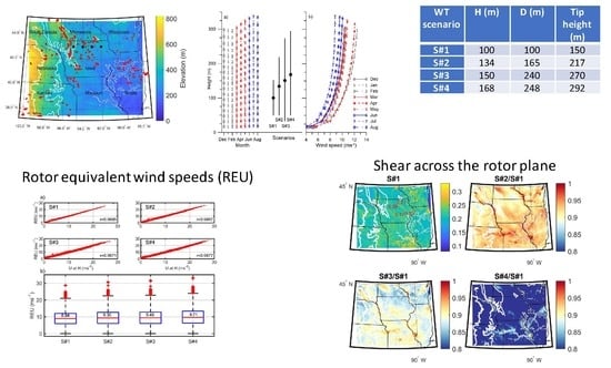
Because WRF employs a terrain-following, dry hydrostatic-pressure coordinate system, the absolute height of each model level above ground varies over the diurnal and seasonal cycle. The conversion from sigma level to height above ground (zh) is done for output from each level in each grid cell at each time step. It is calculated from the perturbation geopotential height (PH), the base geopotential height (PHB) and the mean grid cell elevation above sea level (ELE):
z h = P H + P H B g E L E
where g is acceleration due to gravity.
The model levels are displaced upwards during the warmer months (Figure 3a) due to thermal expansion of the atmospheric column. This variation gives a standard deviation of 5.3% around the long-term mean height at each model level. At the lowest levels, this has a very small impact, e.g., the first model level has a mean of 16.7 m and a standard deviation of 0.9 m, but the deviations increase with height such that for level 18, the mean height and standard deviation around the mean is 315.2 ± 16.6 m.

2.4. WT Scenarios

Four representative scenarios of WT physical dimensions are used here to represent current generation and potential next-generation WT (Table 1 and Figure 3). These WT scenarios are referred to herein as S#x, where x = 1–4. S#1 with H = 100 m and D = 100 m represents an approximation of currently installed WT in the US (H = 90 m, D = 121 m [13]). S#2 (H = 134 m, D = 165 m) is intended to represent the current/next generation of larger turbines similar to the Vestas 150–5.6 MW (D = 150 m) [50] and is slightly larger than the business-as-usual WT [11]. S#3 is based on the IEA Wind 15 MW reference WT (H = 150 m, D = 240 m) [38]. S#3 is slightly larger than both the new Siemens Gamesa 14 MW WT (D = 220 m) [51] and the GE Haliade 12 MW (D = 220 m). S#4 extends both H and D beyond WT that are currently available, i.e., it is a future scenario.
In this analysis, we derive the wind speeds used to compute shear and rotor equivalent wind speed across the rotor plane of each WT scenario (S#x) in each WRF grid cell from the output at each individual model level, thus avoiding any interpolation/extrapolation of the model output. This functionally means that variations in the model layer heights lead to an artificial variation in the implied WT rotor diameter. These monthly variations are relatively modest and equate to maximum variations in implied rotor-swept area of approximately ±10%. Corrections applied for these variations are described below.

2.5. Rotor Equivalent Wind Speed

The rotor equivalent wind speed (REU) is used herein, rather than simply wind speed at hub-height, to fully represent wind speed variation across the rotor plane and to provide an estimate of power output for each WT scenario that fully includes the influence of wind shear across the rotor plane [52,53]. It is computed as [52]:
R E U = i = 1 n h U i 3 A i A 1 / 3
where:
A i = z i z i + 1 c z d z
and
c z = 2 R 2 z H 2
where nh is the number of measurement heights across the rotor plane, Ui is the wind speed measured at the ith height, A is the swept area of the rotor, Ai is the area of the ith rotor segment, zi is the height of the ith segment separation line (1 is the bottom layer), R is the rotor radius and H is the hub-height.

2.6. Power

Power is defined as instantaneous power that is proportional to the cube of the wind speed and the rotor-swept area. Rather than being for a specific wind turbine, the power in the flow across the rotor plane is calculated using Equation (8) that avoids the need for a wind turbine power curve. The power in the flow across the rotor (P in W) at each time step and in each grid cell is computed and aggregated to the calendar month as:
P x , i = 0.5 ρ A x i = 1 n R E U x , i 3
R E U x , i 3 is the cube of the 10-min rotor equivalent wind speeds in each month with n 10-min periods and Ax is the swept area of the rotors in each WT scenario (S#x). This variable is thus not an indication of the expected electrical power production from a given WT but rather the power in the wind over the rotor plane. A normalized power ratio, Prx, for each WT scenario is calculated relative to power output in scenario S#1, such that, e.g., for scenario S#x, the power ratios are:
P r x = ( A x i = 1 n R E U x , i 3 ) / ( A 1 i = 1 n R E U 1 , i 3 )
Prx values are corrected for changes in model level height in each month using the ratio of the mean A computed using all 10-min values to the mean A for that month for a given WT scenario (see the normalized swept areas given in Figure 4). For S#1, the month-to-month variation in A is small, but for the other scenarios, particularly S#3 and S#4, these corrections to Prx are up to 13.5%. In the following, the corrected power ratios are denoted by Pcx.

2.7. Shear across the Rotor Plane

Non-transient wind shear (i.e., timescales of >12 s) is analyzed in accordance with IEC 61400-3 [20]. The shear exponent α across the rotor plane is defined for each 10-min period by Equation (3). If α < 0 or α > 0.2, then shear lies outside the normal operating range. The frequency of negative shear (α < 0) and the frequency of extreme positive shear (α > 0.2) across the rotor plane in each WT scenario and in each WRF grid cell are calculated for all 10-min periods with power producing REU (4–25 ms−1). The frequency of occurrence is expressed relative to the frequency of occurrence in scenario S#1, such that, e.g., for scenario S#x:
S f x = f α x / f ( α 1 )
The magnitude of total wind shear across the rotor plane (Sm, in ms−1/m) for the four WT scenarios is calculated from:
S m = U 2 U 1 / z 2 z 1
where Ux and zx indicate the 10-min wind speeds and height at the top and bottom of the rotor plane (x = 2 at the top of the rotor, and 1 is the bottom). Negative shear is thus defined as occurring when the wind speed at the bottom of the rotor plane exceeds that at the top.
To aid in the interpretation of the vertical wind shear, modeled wind speed profiles are also analyzed to examine the presence of low-level jets (LLJ). In this analysis, once-hourly output from all model levels up to a height of 560 m a.g.l. in each of the four WRF grid cells that comprise the transect are extracted. A wind speed profile is identified as LLJ if the maximum wind speed in any layer within the height interval to 560 m exceeds the wind speed above and below that layer by at least 20% of the maximum. Cases in which a LLJ is identified are analyzed to examine the height of the wind speed maximum at the four locations across the transect.

3. Results

3.1. Wind Speed Profiles and REU

On average, wind speed profiles from all WRF grid cells indicate approximately exponential forms with height, and highest wind speeds at/across WT rotor planes during January and April (Figure 3b). Lower mean wind speeds are simulated for all heights during the summer months. This is consistent with the seasonality observed capacity factors for wind farms within Iowa that also exhibit a summer minimum [54]. Monthly mean wind speed profiles also imply lower shear during summer (Figure 3b).
Median REU and wind speeds at hub-height (U) from the four sites indicate relatively small spatial variability across the transect, but wind speeds in the west have a median REU and U for all four WT scenarios approximately 5% higher than those in the east (Figure 5 and Table 1). Although REU are used in the subsequent analysis, in accordance with Reference [53], differences between median REU and median U are smaller than the site differences, even for the WT scenario using the highest hub-height and largest rotor (Table 1). However, as shown by linear fitting slope and intercept values, there is an increasing divergence between U and REU with increasing H and D (Figure 5).
The probability distribution of 10-min REU values exhibits clear seasonality with higher values and a higher frequency of power-producing wind speeds in winter/spring than summer (Figure 6). However, there are individual periods with high REU in all months. Model output from April and January exhibits the highest mean monthly wind speeds, while April shows a particularly large fraction of 10-min periods with REU above rated wind speeds for typical currently installed WT (~12 ms−1) (Figure 6). Histograms of 10-min REU have slightly flatter probability distributions in the winter/spring months, with more peaked distributions in summer. The probability distributions of REU computed for the WT scenarios with larger H and D are broader and have heavier right tails than in S#1, indicating a greater frequency of high REU (Figure 6).

3.2. Power Ratios

Power in the flow is proportional to the cube of the rotor equivalent wind speed ( R E U 3 ) and to the swept area (A, and hence the square of the rotor diameter) (see Equation (8)). Assuming a shear exponent (α) of 0.2 in Equation (3), the ratio of hub-height wind speed U to S#1 would be 1.06, 1.09 and 1.11 for S#2–S#4 respectively, or 1.19, 1.28 and 1.36 for the ratios of the cubed wind speeds. For constant REU for the four scenarios, the multiplier on the corrected power ratios (Pcx) that derives solely from the increase in swept area would be 2.72, 5.76 and 6.15 for scenarios S#2–S#4, respectively (Figure 4). Thus, the expectations for the mean response to the increase in H and D from the three scenarios (S#2–S#4) are 3.24, 7.37 and 8.36, with the majority of the increase deriving from the increase in the swept area. The computed mean Pcx values derived using WRF output for all 10-min periods to compute the REU are: 3.29–3.30 for S#2 at the four transect locations, 7.00 to 7.10 for S#3 and 8.38 to 8.73 for S#4. Thus, there is broad but incomplete agreement between the a priori expectations and the model-derived values. However, for the largest WT considered, the modeled increase in the mean wind power across the rotor plane exceeds that estimated using the power law wind speed profile (Equation (2)), with α = 0.2. This might imply that the rotor plane is no longer contained wholly within the surface layer.
Temporal variability in Pcx shown in Table 2 arises due to deviations of the wind profile from the expectation based on surface scaling laws with a constant α. Table 2 indicates that mean Pcx values vary modestly across the transect. The transect-wise variability is lower than the temporal variability at each location, as manifest by the standard deviation of the 10-min values (Table 2). However, there is evidence of lesser enhancement of Pcx for the larger rotors (S#3 and S#4) and of lower month-to-month variability in Pcx values at the eastern sites (Table 2). This implies there may be important spatial variability in the wind speed profile with height across the transect.
There is pronounced seasonal variability in normalized REU and power in the flow (P and Pcx) for the four WT scenarios (where each is corrected for the seasonality in WRF layer heights). Values are lowest in summer, consistent with deeper boundary layers and lower levels of wind shear during the summer months (Figure 4). The standard deviation of monthly power estimates for WT scenario S#4 is 53% of the mean of the monthly values, with January and April exhibiting particularly high power while the month of July exhibits the lowest power (Table 3).

3.3. Shear across the Rotor Plane

The model-derived shear exponent across the rotor plane (α) is frequently greater than 0.2 at all four locations on the transect, and across the whole domain, irrespective of the WT scenario under consideration (Figure 7, Table 3).
The domain average α computed for all 10-min time periods for WT S#1 (that broadly represents WT currently being deployed and has H = 100 m, D = 100 m) is 0.21 ± 0.02. For S#1, the shear exponent derived from model output for 50 to 150 m over parts of Lake Michigan (east of Wisconsin) is very low (~0.08), but for most areas, the temporal mean α is between 0.2 and 0.3 (Figure 7a). Some areas such as the metropolitan area of Chicago (northeast Illinois) and the forested areas in the southwest of Wisconsin and southeast of Missouri have higher temporal mean values up to 0.33 (Figure 7a). For comparison, measurements across the height range 50–150 m from four tall towers in Iowa conducted during December 2006–January 2009 at Palmer (flat rural), Mason City (flat, rural/urban); Altoona (flat, suburban) and Homestead (hilly, rural) [23] indicate approximate average annual shear exponents of 0.17 for Altoona, 0.22 at Homestead, 0.24 at Mason City and 0.28 at Palmer (see locations shown by the red markers in Figure 7a) [23]. Those data indicate somewhat larger seasonal and spatial variability in α than is evident in the WRF output (Figure 7a and Figure 8a). Shear exponents from WRF likely indicate less variability than those from observations due to sub-grid scale effects arising from land use land cover and topographic variability since modeled wind shear is known to be sensitive to the land surface model used in WRF and the land cover datasets employed [55].
Analyses of WRF output for the biggest turbine scenario (S#4) indicates substantially smaller mean shear exponent values than S#1 (Figure 7) due to the swept area generally extending less close to the ground surface and thus avoiding the most sheared layer of the atmosphere (Figure 3b). Time and domain average shear exponents decrease to 0.198, 0.191 and 0.166 for S#2, S#3 and S#4, respectively. Very few grid cells experience mean values of the ratio α S # x α S # 1 (where x is 2, 3, 4 for S#2, S#3 and S#4) that exceed 1 (Figure 7b–d). Thus, every scenario with a larger rotor and taller hub-height experiences overall lower wind shear across the rotor plane. Areas in the domain with high shear exponent ratios are mainly along river valleys, while over the remainder of the domain the ratios are <1. S#2 and S#4 have the most spatially homogeneous shear exponent fields. S#3 shows higher spatial variability, likely because in this scenario the lowest height included is model layer 2, whereas the other scenarios use model layer 3 as the lowest height from which the shear exponent is calculated.
There is seasonal variability in vertical shear exponents. Observations from December 2006–January 2009 from Palmer, Mason City, Altoona and Homestead indicate that shear exponents are highest in winter and lowest in summer [23]. Consistent with those data, WRF output for the winter months generally exhibit highest shear exponent values across the rotor plane, irrespective of the precise WT scenario (Table 3). For example, domain-wide mean values are lowest in April for WT S#1, which is also a high wind speed month (Figure 3b) and are higher during the winter months and August (Table 3). In April, there is a marked transition in turbulence kinetic energy levels from low levels in winter, to higher turbulence kinetic energy levels in summer, indicating a decrease in wind shear associated with more convective conditions [47]. Lowest shear exponent values are derived for the WT scenario #4 during June and July rather than April.
The shear exponent derived from the WRF output also shows a marked diurnal cycle with lowest values during the day at all locations on the transect, consistent with the presence of buoyancy-derived vertical mixing (convection) during the daytime, and a greater prevalence of statically stable conditions and higher REU at night (Figure 8). This seasonal and diurnal variability in shear exponent is also evident in tall tower measurements for four sites in Iowa (locations shown in Figure 7a), where mean seasonal values by hour of the day range from 0.19 to 0.55 overnight, to 0.02 to 0.2 during the daytime [23]. Consistent with the mean monthly values from WRF, shear exponents are systematically higher in winter than in summer. This comparison of model-derived shear exponents with a completely independent measurement set from tall tower measurements gives confidence that the WRF simulations are reproducing the shear over the rotor plane.
Observational research has indicated a high frequency of extreme positive shear in Iowa [36]. Using criteria for “challenging flow conditions’’ for turbine operations within the rotor layer when the mean hub wind speed is between 8 and 13 ms−1, the layer is critically stable (0 < Ri < 0.25), where Ri is Richardson number and the power-law exponent is larger than 0.2). We find that the Iowa sites experienced such conditions approximately 25% of the time (37% for Altoona, 26% for Homestead, 26% for Mason City, 22% for Palmer) [23].
Output from the WRF simulation at the four locations on the transect also indicate a high frequency of occurrence of high shear exponent (α > 0.2). Individual calendar months have α > 0.2 frequency that ranges from 34% to 66% for WT S#1 and is between 24% and 66% for all WT scenarios. In other words, high shear α > 0.2 occurs more than 24% of the time in every month, for all four WT scenarios and at all of the four transect locations (Figure 9). High shear is most frequent in December and January and there is a noticeable decrease in the frequency of occurrence of extreme positive shear at the four WRF locations from April to July (Figure 9), with a minimum frequency of α > 0.2 of 24% in July for S#4. Extreme positive shear exponents are less frequent in the WT scenarios, with larger H and D than in S#1, but remain common. The mean frequencies of α > 0.2 averaged over all calendar months across the four locations for the four WT scenarios are S#1 = 47.9%, S#2 = 45.8%, S#3 = 44.5% and S#4 = 37.8%. The differences in shear occurrence on the transect also vary by month, less so in December and January when the frequency is fairly consistent (within 7%) between the four sites. The eastern-most site (92° W) has more frequent high shear than the western site (95° W) in June, July and August in every scenario (Figure 9).
Shear exponents computed from model output are most likely to be high overnight and during winter. For S#1, 70% of α values in excess of the 90th percentile value occurred between 22:00 and 6:00 h (local time). However, during July and August, high shear values are most prevalent during early morning from 6:00 to 8:00 h (local time). For the other WT scenarios, winter months also show the highest frequency of high shear cases and a bias towards occurrence between 22:00 and 6:00. However, the occurrence of high shear events is less focused on these nighttime hours, and the months with the highest frequency of extreme positive shear are January, March and August, which may indicate that for the larger rotors and higher H, the occurrence of extreme shear is not solely a product of nocturnal stabilization of the surface layer. This may indicate that the extension to greater heights gives more frequent interaction between the rotor plane and the low-level jet (LLJ) and that is a cause of the increase in extreme positive shear for WT S#3 and S#4. The mean height of the LLJ (defined as the height of a maximum of wind speeds between 30 and 560 m height, which is at least 20% greater than the wind speeds above and below it) at the four transect locations is 181–189 m (Table 4). The LLJ maximum is thus frequently within the rotor plane of the WT employed in S#3 and S#4 when the upper rotor tip extends to 270 and 292 m above the ground.
Causes of high shear include more stable conditions, the presence of topographic flows and/or low turbulence and vertical mixing and the occurrence of LLJ. The western site has more complex topography (Figure 2) and overall the highest shear exponent (Figure 7 and Figure 8), but it does not uniformly experience the greatest frequency of α > 0.2. In the summer months when conditions are most unstable (convective) and wind speeds are lowest [46], the eastern sites tend to experience high shear more frequently. The regional flow is generally dominated by southeasterly and southwesterly flow in winter and spring and dominated by southwesterly flow in summer [54]. The LLJ is more frequently associated with north/south wind directions and is more common in the northeast of the domain in spring [31] and may account for the high frequency of extreme shear in March and at night.
Negative wind shear exponents computed across the rotor plane are substantially less frequently observed than extreme positive shear and have modest magnitudes, although α < 0 is most commonly observed for the largest rotor (Figure 10). Indeed, many of the negative shear periods might reasonably be presented as no-shear profiles (i.e., α ~ 0) (Figure 10 and Figure 11) rather than associated with a LLJ [32]. Nevertheless, the model simulations indicate negative wind shear overnight, particularly during low wind speed (summer) months (Figure 10). For site 1, S#1, 64% of 10-min periods that are characterized by negative shear exponents occur during 22:00–7:00 h. Increasing both H and D increases the frequency of negative shear, particularly for S#4 (Figure 10b).
Thus, to summarize, the shear exponent computed across the rotor planes for each of the WT scenarios frequently falls within the IEC expected range (0–0.2). However, as indicated in Figure 11, the shear exponent across the rotor plane for the four WT scenarios is repeatedly outside of this range. High shear (α > 0.2) occurs more frequently at power-producing wind speeds than does negative shear, although it is most frequent when wind speeds are lower than typical rated wind speeds (12–15 ms−1). As H and D increase (i.e., moving from WT scenario S#1 to S#4), the frequency of extreme positive shear is projected to decrease. For example, at the most westerly site on the transect over northern Iowa (location 1: 95° W), the frequency with which the wind shear exponent across the blade exceeds 0.2 decreases from 48% of 10-min periods to 38% of periods from WT S#1 to WT S#4. Also, the occurrence of high absolute shear values (expressed in ms−1/m) declines at virtually all hub-height wind speeds (Figure 11). Although there is a small increase in the frequency of occurrence of negative shear across the rotor plane with increasing H and D, the majority of negative shear exponents are of very small magnitude and thus are perhaps more properly described as close to zero.

4. Discussion and Concluding Remarks

In principle, the current wind energy industry trend towards larger turbines with higher hub-height (H) and larger rotor diameter (D) (Figure 1) should yield electrical power production gains due to the increase in swept area and typical increase of wind speeds with height. However, the vertical profiles of wind speeds above the surface layer can be very complex [25,26], particularly in heterogeneous terrain and landscapes, potentially leading to only modest increases in rotor equivalent wind speeds and/or increased fatigue loading due to the increased prevalence of extreme shear across the rotor plane. The impact of increasing WT dimensions on both the energy content of the flow (power) and wind shear across the rotor plane is examined using output from high-resolution simulations with WRF performed for a domain centered on the US state of Iowa for December 2007–August 2008. This region of the US has high wind resources and a high density of WT installed capacity but is also known to exhibit complex and highly sheared wind speed profiles.
Four scenarios of WT hub-height and rotor diameter were considered. Scenario S#1 broadly represents the dimensions of WT that are currently being installed: H = 100 m, D = 100 m. In scenario S#2: H = 134 m, D = 165 m. In scenario S#3: H = 150 m, D = 240 m. While in scenario S#4: H = 168 m, D = 248 m. Thus, scenarios 2 and 3 represent approximations of WT that are on the market currently—S#2 approximates the Vestas 150–5.6 MW and is slightly larger than the business-as-usual WT [11]. S#3 is based on the IEA Wind 15 MW reference turbine (H = 150 m, D = 240 m) [38], while S#4 extends both H and D beyond WT that are currently available but is intended to represent a plausible future WT design.
It is important to acknowledge that other constraints may limit the continued growth (up-sizing) of WT. These include declines in social acceptance due to factors such as increased turbine visibility [56], limitations imposed by set-back regulations [57] and/or additional permitting requirements for larger turbines such as those from the US Federal Aviation Authority for WT that have rotor tip heights above 499 ft (152 m). There are other logistics and engineering constraints on turbine up-scaling, particularly for onshore deployments, linked to manufacturing, transportation and costs [11,58]. Further, some causes of atmospheric flow variability will be sub-grid scale in the simulations presented herein. Thus, future work should include long-term simulations with WRF applied at even higher resolution and/or use of micro-scale models including large eddy simulation (LES) [59,60] to confirm inferences presented herein regarding the relative benefits of deployment of WT with larger physical dimensions.
There are substantial gains implied in terms of the energy content of the flow across the rotor plane from increasing the hub-height or increasing the size of the rotor plane such that the top tip extends to over 200 m. Expected power gains based purely on the theoretical increase of swept area from increased rotor diameter in the four scenarios expressed as a ratio to S#1 are 1, 2.72, 5.76 and 6.15. Expected power gains based purely on the increase in wind speed from increased hub-height (using the power law Equation (2) with a shear exponent of 0.2) in the four scenarios expressed as a ratio to S#1 are 1, 1.19, 1.28 and 1.36. Thus, the theoretical increase in power for the four scenarios expressed as a ratio to S#1 are 1, 3.24, 7.37 and 8.36.
Analyses of output from WRF simulations performed over a 9-month period with a horizontal grid spacing of 4 km and 57 vertical levels suggest that the rotor equivalent wind speed (REU) is well-represented by the median wind speed but that divergence between these values increases as the turbine dimensions increase. The power ratios calculated from WRF output for the four scenarios expressed as a ratio to S#1 are 1, 3.30, 7.08 and 8.73. These compare favorably with the theoretical values, with the slightly lower values in S#2 arising from lower wind speeds in model layer 2 while S#4 has slightly greater power than predicted. Monthly variability in REU is consistent across the scenarios, giving highest power in January and April and lowest in July and August.
Deployment of larger WT in the eastern central plains may result in only small penalties in terms of the frequency of occurrence of extreme positive or negative wind shear across the rotor plane that may impact turbine loading [33]. The WRF-derived average shear exponent α across the rotor plane is 0.21 for S#1, consistent with observations from three sites in central/eastern Iowa and lower than the Iowa site in more complex terrain (α = 0.28 at Palmer). Output from the 4 km WRF model simulations indicates a high frequency (48%) of extreme positive shear (α > 0.2) across the WT rotor at power-producing wind speeds. The occurrence of negative shear is low (<12% for any scenario at any site) but increases from 4.2% to 6.2% for S#1–3 to nearly 12% for the largest wind turbine scenario (S#4). High shear occurs particularly overnight and during the winter months (in agreement with observations). The frequency of occurrence of high shear exponents (α > 0.2) declines with increasing H and D over virtually all of the domain. For the largest wind turbine considered, the frequency of high shear decreases to 38% for the most western site for scenario S#1. The mean height of the LLJ computed from the WRF output is around 185 m. Thus, increasing the top-tip height in the scenarios increases the frequency with which the LLJ impinges on the rotor plane. At the four transect locations, the LLJ frequency increases from 7.7% to 9.0% in WT scenario S#1 to 18.2% to 19.2% for S#4.
Although detailed modeling should be conducted to quantify the load implications on WT, the modeled response to increases in WT dimensions indicates substantial power gains and a decrease in the frequency of high positive shear across the rotor plane.

Author Contributions

R.J.B. conceived the research concept. R.J.B. and S.C.P. jointly developed the analysis strategy. T.J.S. ran the simulations. J.A.A. analyzed the model output for LLJ. R.J.B. and S.C.P. wrote the manuscript with input from T.J.S. and J.A.A. All authors have read and agreed to the published version of the manuscript.

Funding

This work was support by the US Department of Energy (DoE) (DE-SC0016438 and DE-SC0016605). The research used computing resources from the National Science Foundation: Extreme Science and Engineering Discovery Environment (XSEDE) (allocation award to SCP is TG-ATM170024).

Acknowledgments

We gratefully acknowledge the helpful comments and suggestions of three reviewers.

Conflicts of Interest

The authors declare no conflict of interest

References

  1. WindEurope. Wind Energy in Europe Trends and Statistics 2019. p. 24. Available online: https://windeurope.org/wp-content/uploads/files/about-wind/statistics/WindEurope-Annual-Statistics-2019.pdf (accessed on 27 February 2020).
  2. WindEurope. Offshore Wind in Europe Key Trends and Statistics 2019. p. 40. Available online: https://windeurope.org/wp-content/uploads/files/about-wind/statistics/WindEurope-Annual-Offshore-Statistics-2019.pdf (accessed on 27 February 2020).
  3. Hand, M.M. (Ed.) IEA Wind TCP Task 26‒Wind Technology, Cost, and Performance Trends in Denmark, Germany, Ireland, Norway, Sweden, the European Union, and the United States: 2008‒2016; NREL/TP-6A20.71844; National Renewable Energy Laboratory: Golden, CO, USA, 2008; p. 104. Available online: https://www.nrel.gov/docs/fy19osti/71844.pdf (accessed on 13 July 2020).
  4. Wiser, R.; Bolinger, M. 2018 Wind Technologies Market Report; DOE/GO-102019-5191; U.S. Department of Energy, Office of Energy Efficiency and Renewable Energy: Oak Ridge, TN, USA, 2018; p. 103. Available online: https://www.energy.gov/eere/wind/downloads/2018-wind-technologies-market-report (accessed on 13 August 2020).
  5. Bolinger, M.; Lantz, E.; Wiser, R.; Hoen, B.; Rand, J.; Hammond, R. Opportunities for and challenges to further reductions in the “specific power” rating of wind turbines installed in the United States. Wind Eng. 2020. [Google Scholar] [CrossRef] [Green Version]
  6. IRENA. Future of Wind Deployment, Investment, Technology, Grid Integration and Socio-Economic Aspects; International Renewable Energy Agency: Abu Dhabi, UAE, 2019; p. 88. ISBN 978-92-9260-155-3. [Google Scholar]
  7. WindEurope. Wind Energy in Europe: Outlook to 2023. 2019, p. 40. Available online: https://www.anev.org/wp-content/uploads/2019/10/Market-outlook-2019.pdf (accessed on 13 August 2020).
  8. Beiter, P.; Musial, W.; Kilcher, L.; Maness, M.; Smith, A. An Assessment of the Economic Potential of Offshore Wind in the United States from 2015 to 2030; Technical Report: NREL/TP-6A20-67675; National Renewable Energy Laboratory: Golden, CO, USA, 2017; p. 77.
  9. Preindl, M.; Bolognani, S. Optimization of the generator to rotor ratio of mw wind turbines based on the cost of energy with focus on low wind speeds. In Proceedings of the IECON 2011 37th Annual Conference of the IEEE Industrial Electronics Society, Victoria, Australia, 7–10 November 2011; pp. 906–911. [Google Scholar]
  10. Wiser, R.; Millstein, D.; Bolinger, M.; Jeong, S.; Mills, A. The hidden value of large-rotor, tall-tower wind turbines in the United States. Wind Eng. 2020. [Google Scholar] [CrossRef]
  11. Lantz, E.; Roberts, O.; Nunemaker, J.; DeMeo, O.; Dykes, K.; Scott, G. Increasing Wind Turbine Tower Heights: Opportunities and Challenges; NREL/TP-5000-73629; National Renewable Energy Laboratory: Golden, CO, USA, 2019; p. 66.
  12. Musial, W.; Beiter, J.; Spitsen, P.; Nunemaker, J.; Gevorgian, V. 2018 Offshore Wind Technologies Market Report; Department of Energy: Oak Ridge, TN, USA, 2019; p. 94. [Google Scholar]
  13. AWEA. Wind Powers America. 2019 Annual Report; American Wind Energy Association: Washington, WA, USA, 2020; p. 138. [Google Scholar]
  14. AWEA. AWEA Wind IQ. Available online: https://windiq.awea.org/app/ (accessed on 26 May 2020).
  15. IEA. Offshore Wind Outlook; IEA: Paris, France, 2019; p. 98. [Google Scholar]
  16. Stull, R.B. An Introduction to Boundary Layer Meteorology; Kluwer Publications Ltd.: Dordrecht, The Netherlands, 1988; p. 666. ISBN 90-277-2768-6. [Google Scholar]
  17. Foken, T. 50 years of the Monin–Obukhov similarity theory. Bound. Layer Meteorol. 2006, 119, 431–447. [Google Scholar] [CrossRef]
  18. Motta, M.; Barthelmie, R.J.; Vølund, P. The influence of non-logarithmic wind speed profiles on potential power output at Danish offshore sites. Wind Energy 2005, 8, 219–236. [Google Scholar] [CrossRef]
  19. Irwin, J.S. A theoretical variation of the wind profile power-law exponent as a function of surface roughness and stability. Atmos. Environ. 1979, 13, 191–194. [Google Scholar]
  20. International Electrotechnical Commission. International Standard, IEC61400 Wind Turbines Wind Energy Generation Systems–Part 1: Design Requirements, Edition 4.0 2019-02; IEC, FDIS: Geneva, Switzerland, 2019; p. 172. [Google Scholar]
  21. Drechsel, S.; Mayr, G.J.; Messner, J.W.; Stauffer, R. Wind Speeds at Heights Crucial for Wind Energy: Measurements and Verification of Forecasts. J. Appl. Meteorol. Climatol. 2012, 51, 1602–1617. [Google Scholar] [CrossRef]
  22. Schwartz, M.; Elliott, D. Wind Shear Characteristics at Central Plains Tall Towers; NREL/CP-500-40019; National Renewable Energy Laboratory: Golden, CO, USA, 2006; p. 10.
  23. Walton, R.A.; Takle, E.S.; Gallus, W.A. Characeristics of 50-200m winds and temperatures derived from an Iowa tall-tower network. J. Appl. Meteorol. Climatol. 2014, 53, 2387–2393. [Google Scholar] [CrossRef] [Green Version]
  24. Gryning, S.E.; Batchvarova, E.; Brümmer, B.; Jørgensen, H.E.; Larsen, S.E. On the extension of the wind profile over homogeneous terrain beyond the surface boundary layer. Bound. Layer Meteorol. 2007, 124, 251–268. [Google Scholar]
  25. Peña, A.; Gryning, S.E.; Mann, J. On the length-scale of the wind profile. Q. J. R. Meteorol. Soc. 2010, 136, 2119–2131. [Google Scholar] [CrossRef]
  26. Sathe, A.; Gryning, S.-E.; Peña, A. Comparison of the atmospheric stability and wind profiles at two wind farm sites over a long marine fetch in the North Sea. Wind Energy 2011, 14, 767–780. [Google Scholar] [CrossRef]
  27. Shapiro, A.; Fedorovich, E. Analytical description of a nocturnal low-level jet. Q. J. R. Meteorol. Soc. 2010, 136, 1255–1262. [Google Scholar] [CrossRef]
  28. Storm, B.; Basu, S. The WRF model forecast-derived low-level wind shear climatology over the United States Great Plains. Energies 2010, 3, 258–276. [Google Scholar] [CrossRef]
  29. Nikolic, J.; Zhong, S.; Pei, L.; Bian, X.; Heilman, J.; Charney, J.J. Sensitivity of Low-Level Jets to Land-Use and Land-Cover Change over the Continental U.S. Atmosphere 2019, 10, 174. [Google Scholar] [CrossRef] [Green Version]
  30. Storm, B.; Dudhia, J.; Basu, S.; Swift, A.; Giammanco, I. Evaluation of the Weather Research and Forecasting model on forecasting low-level jets: Implications for wind energy. Wind Energy 2009, 12, 81–90. [Google Scholar] [CrossRef]
  31. Aird, J.A.; Barthelmie, R.J.; Shepherd, T.J.; Pryor, S.C. WRF-Simulated springtime low-level jets over Iowa: Implications for Wind Energy. J. Phys. Conf. Ser. Sci. Mak. Torque Wind. 2020, in press. [Google Scholar]
  32. Gutierrez, W.; Ruiz-Columbie, A.; Tutkun, M.; Castillo, L. Impacts of the low-level jet’s negative wind shear on the wind turbine. Wind Energ. Sci. 2017, 2, 533–545. [Google Scholar] [CrossRef] [Green Version]
  33. Robertson, A.N.; Shaler, K.; Sethuraman, L.; Jonkman, J. Sensitivity analysis of the effect of wind characteristics and turbine properties on wind turbine loads. Wind Energ. Sci. 2019, 4, 479–513. [Google Scholar] [CrossRef] [Green Version]
  34. Park, J.; Basu, S.; Manuel, L. Large-eddy simulation of stable boundary layer turbulence and estimation of associated wind turbine loads. Wind Energy 2014, 17, 359–384. [Google Scholar] [CrossRef]
  35. Smith, K.; Randall, G.; Malcolm, D. Evaluation of Wind Shear Patterns at Midwest Wind Energy Facilities; NREL: Golden, CO, USA, 2002; p. 20. Available online: https://www.nrel.gov/docs/fy02osti/32492.pdf (accessed on 13 August 2020).
  36. Barthelmie, R.J.; Shepherd, T.J.; Pryor, S.C. Increasing turbine dimensions: Impact on shear and power. J. Phys. Conf. Ser. Sci. Mak. Torque Wind. 2020, 2020, 10. [Google Scholar]
  37. Rand, J.T.; Kramer, L.A.; Garrity, C.P.; Hoen, B.D.; Diffendorfer, J.E.; Hunt, H.E.; Spears, M. A continuously updated, geospatially rectified database of utility-scale wind turbines in the United States. Sci. Data 2020, 7, 1–12. [Google Scholar] [CrossRef]
  38. Gaertner, E.; Rinker, J.; Sethuraman, L.; Zahle, Z.; Anderson, B.; Barter, G.; Abbas, B.; Meng, F.; Bortolotti, F.; Skrzypinski, W.; et al. Definition of the IEA 15-Megawatt Offshore Reference Wind; NREL/TP-5000-75698; National Renewable Energy Laboratory: Golden, CO, USA, 2020. Available online: https://www.nrel.gov/docs/fy20osti/75698.pdf (accessed on 13 August 2020).
  39. Mann, J.; Angelou, N.; Arnqvist, J.; Callies, D.; Cantero, E.; Arroyo, R.C.; Courtney, M.; Cuxart, J.; Dellwik, E.; Gottschall, J.; et al. Complex terrain experiments in the New European Wind Atlas. Philos. Trans. R. Soc. A Math. Phys. Eng. Sci. 2017, 375. [Google Scholar] [CrossRef] [PubMed]
  40. Wilczak, J.M.; Olson, J.B.; Djalalova, I.; Bianco, L.; Berg, L.K.; Shaw, W.J.; Coulter, R.L.; Eckman, R.M.; Freedman, J.; Finley, C.; et al. Data assimilation impact of in situ and remote sensing meteorological observations on wind power forecasts during the first Wind Forecast Improvement Project (WFIP). Wind Energy 2019, 22, 932–944. [Google Scholar] [CrossRef] [Green Version]
  41. Letson, F.; Barthelmie, R.J.; Hu, W.; Pryor, S.C. Characterizing wind gusts in complex terrain. Atmos. Chem. Phys. 2019, 19, 3797–3819. [Google Scholar] [CrossRef] [Green Version]
  42. Barthelmie, R.J.; Pryor, S.C. Automated wind turbine wake characterization in complex terrain. Atmos. Meas. Tech. 2019, 12, 3463–3484. [Google Scholar] [CrossRef] [Green Version]
  43. Guggeri, A.; Draper, M. Large Eddy Simulation of an Onshore Wind Farm with the Actuator Line Model Including Wind Turbine’s Control below and above Rated Wind Speed. Energies 2019, 12, 3508. [Google Scholar] [CrossRef] [Green Version]
  44. Cheng, W.Y.; Liu, Y.; Bourgeois, A.J.; Wu, Y.; Haupt, S.E. Short-term wind forecast of a data assimilation/weather forecasting system with wind turbine anemometer measurement assimilation. Renew. Energy 2017, 107, 340–351. [Google Scholar] [CrossRef]
  45. Hahmann, A.N.; Sıle, T.; Witha, B.; Davis, N.N.; Dörenkämper, M.; Ezber, Y.; García-Bustamante, E.; González-Rouco, J.F.; Navarro, J.; Olsen, B.T. The making of the New European Wind Atlas, Part 1: Model sensitivity. Geosci. Model Dev. Discuss. 2020. in review. Available online: https://doi.org/10.5194/gmd-2019-349 (accessed on 13 August 2020).
  46. Hahmann, A.N.; Vincent, C.L.; Peña, A.; Lange, J.; Hasager, C.B. Wind climate estimation using WRF model output: Method and model sensitivities over the sea. Int. J. Climatol. 2015, 35, 3422–3439. [Google Scholar] [CrossRef]
  47. Pryor, S.C.; Shepherd, T.J.; Volker, P.J.; Hahmann, A.N.; Barthelmie, R.J. ‘Wind theft’ from onshore arrays: Sensitivity to wind farm parameterization and resolution. J. Appl. Meteorol. Climatol. 2020, 59, 153–174. [Google Scholar] [CrossRef]
  48. Pryor, S.C.; Shepherd, T.J.; Volker, P.J.H.; Hahmann, A.N.; Barthelmie, R.J. Diagnosing systematic differences in predicted wind turbine array-array interactions. J. Phys. Conf. Ser. Sci. Mak. Torque Wind 2020, in press. [Google Scholar]
  49. Pryor, S.C.; Shepherd, T.J.; Barthelmie, R.J.; Hahmann, A.N.; Volker, P.J.H. Wind farm wakes simulated using WRF. J. Phys. Conf. Ser. 2019, 1256, 012025. [Google Scholar]
  50. Vestas. EnVentus™ V150-5.6 MW™ IEC S. Available online: https://www.vestas.com/en/products/enventus_platform/v150%205_6_mw#!grid_0_content_6_Container (accessed on 20 May 2020).
  51. Wind Energy Update. Siemens Gamesa to Deploy 14 MW Offshore Turbines by 2024. Available online: https://analysis.newenergyupdate.com/wind-energy-update/siemens-gamesa-unveils-giant-14-mw-turbine-new-england-study-favors-shared?utm_campaign=NEP%20WIN%2020MAY20%20Newsletter%20B&utm_medium=email&utm_source=Eloqua&elqTrackId=afe60f99cc1f473f9504c76c66ed4570&elq=ad7880b7461f4aa68b5fe4d257986140&elqaid=53488&elqat=1&elqCampaignId=34426 (accessed on 20 May 2020).
  52. Wagner, R.; Cañadillas, B.; Clifton, A.; Feeney, S.; Nygaard, N.; Poodt, M.; St. Martin, C.; Tüxen, E.; Wagenaar, J.W. Rotor equivalent wind speed for power curve measurement-comparative exercise for IEA Wind Annex 32. J. Phys. Conf. Ser. 2014, 524, 012108. [Google Scholar] [CrossRef]
  53. Van Sark, W.; Van der Velde, H.C.; Coelingh, J.P.; Bierbooms, W. Do we really need rotor equivalent wind speed? Wind Energy 2019, 22, 745–763. [Google Scholar] [CrossRef] [Green Version]
  54. Shepherd, T.J.; Barthelmie, R.J.; Pryor, S.C. Sensitivity of wind turbine array downstream effects to the parameterization used in WRF. J. Appl. Meteorol. Climatol. 2020, 59, 333–361. [Google Scholar] [CrossRef]
  55. Wharton, S.; Simpson, M.; Osuna, J.L.; Newman, J.F.; Biraud, S.C. Role of Surface Energy Exchange for Simulating Wind Turbine Inflow: A Case Study in the Southern Great Plains, USA. Atmosphere 2015, 6, 21–49. [Google Scholar] [CrossRef] [Green Version]
  56. Enevoldsen, P.; Sovacool, B.K. Examining the social acceptance of wind energy: Practical guidelines for onshore wind project development in France. Renew. Sustain. Energy Rev. 2016, 53, 178–184. [Google Scholar] [CrossRef]
  57. Meyerhoff, J.; Ohl, C.; Hartje, V. Landscape externalities from onshore wind power. Energy Policy 2010, 38, 82–92. [Google Scholar] [CrossRef]
  58. McKenna, R.; vd Leye, P.O.; Fichtner, W. Key challenges and prospects for large wind turbines. Renew. Sustain. Energy Rev. 2016, 53, 1212–1221. [Google Scholar] [CrossRef]
  59. Haupt, S.E.; Kosovic, B.; Shaw, W.; Berg, L.K.; Churchfield, M.; Cline, J.; Draxl, C.; Ennis, B.; Koo, E.; Kotamarthi, R. On bridging a modeling scale gap: Mesoscale to microscale coupling for wind energy. Bull. Am. Meteorol. Soc. 2019, 100, 2533–2550. [Google Scholar] [CrossRef]
  60. Mirocha, J.D.; Churchfield, M.J.; Muñoz-Esparza, D.; Rai, R.K.; Feng, Y.; Kosović, B.; Haupt, S.E.; Brown, B.; Ennis, B.L.; Draxl, C.; et al. Large-eddy simulation sensitivities to variations of configuration and forcing parameters in canonical boundary-layer flows for wind energy applications. Wind Energ. Sci. 2018, 3, 589–613. [Google Scholar] [CrossRef] [Green Version]
Figure 1. (a) Mean hub-height (H, in m) and (b) rotor diameter (D, in m) and rated capacity (RC, in megawatts (MW), symbol size) of wind turbines (WT) installed in each calendar year in the EU to 2015, and USA and offshore to 2018 [3,4,5]. WT dimensions from 2019 onwards are projections shown by the open symbols [6,7,8]. The line in the left panel shows annual mean capacity factors in the US from 2008 to 2015 [4].
Energies 13 04269 g001
Figure 2. Map of the terrain elevation within the inner Weather Research and Forecasting (WRF) domain that is described using 4 × 4 km grid cells. The black lines show the state boundaries, and the white lines show terrain contours at 200 m (thinnest), 400 m and 600 m (thickest) used to denote the topography. The locations of individual WT are shown in red. These are from https://eerscmap.usgs.gov/uswtdb/ updated 14 May 2020 [37]. The location of the four sites on the transect at 43° N latitude across the north of Iowa are shown by the black circles.
Energies 13 04269 g002
Figure 3. (a) Mean model levels (shown by the numbers) in the WRF output for each calendar month derived from the modeled sigma coordinate system. The solid black lines show the hub-height and top and bottom of the rotor plane for each of the four WT scenarios, S#x (i.e., variations of H and D, see Table 1). (b) Mean wind speed profile at site 1: 43° N, 95° W, in each calendar month computed using 10-min output from the lowest 18 model levels where the numbers depict the mean height of each model level.
Energies 13 04269 g003
Figure 4. Normalized swept area of the rotor (A) for each WT scenario relative to S#1 by calendar month (sold lines). Mean Prx for each WT scenario is shown as the solid line with the triangle symbol. Mean Pcx in each calendar month corrected for the variation in A is shown by the squares. There is little spatial variability in the variations of A by month, thus A, Prx and Pcx values shown here are a mean of those from the four sites across the transect.
Energies 13 04269 g004
Figure 5. (a) Four scatterplots showing the rotor equivalent wind speed (REU) vs. hub-height median wind speeds for the WT scenarios S#1–S#4 for Site 1. The numbers in the lower right corner of each sub-panel are the Pearson correlation coefficient (r), the slope (m) and the intercept (c). (b) Box-whisker plot showing median, 25% and 75% quartiles (the limits on the boxes) of 10-min REU for the four WT scenarios at site 1. Whiskers extend to the 1st to 99th percentile values of REU (ms−1). The number in the center of the box indicates median hub-height wind speeds for each WT scenario.
Energies 13 04269 g005
Figure 6. Histograms of 10-min REU discretized in 4 ms−1 wind speed classes as sampled by climatological season (colors) and the four WT scenarios (panels (ad)). The REU shown are for the most westerly location Site 1 (43° N, 95° W).
Energies 13 04269 g006
Figure 7. Shear exponent α for the four WT scenarios. The top left panel shows α calculated for each grid cell for the period December 2017–August 2018 for S#1. The other panels show the ratio of the mean shear exponent for S#2, S#3 and S#4 relative to the first scenario. The color bars for panels (bd) have been restricted to 0–1 to aid legibility and comparison of the four scenarios. Observationally derived estimates of annual mean shear exponent from tall towers in Iowa for December 2006–January 2009 are also shown in (a). These estimates are of 0.17 for Altoona, 0.22 at Homestead, 0.21 at Mason City and 0.28 at Palmer, and are shown by the red numbers in (a) [23]. The black lines show the state boundaries, and the white lines show terrain contours at 200 m (thinnest), 400 m and 600 m (thickest) used to denote the topography.
Energies 13 04269 g007
Figure 8. (a) Diurnal variability of the shear exponent over the layer from 50–150 m from WRF for the four transect sites and measurements at four sites in Iowa as reported in Reference [23]. (b) Diurnal variability of REU based on output from WRF for the four transect locations and four WT scenarios.
Energies 13 04269 g008
Figure 9. The frequency of shear exponent α > 0.2 at the four transect sites shown by longitude (latitude = 43° N) and for the four WT scenarios. The center value in red is the frequency in S#1 (%). The colored circles show the frequency as a ratio α S # x α S # 1 , where S#2 is blue, S#3 is cyan and S#4 is black. The minimum ratio is 0.59 (site 95° W, S#4 in July) and the maximum is 1.04 (site 93° W, S#3 in August).
Energies 13 04269 g009
Figure 10. Negative shear: (a) The diurnal frequency (number of hours) and shear exponent α for negative shear hours at S#4, Site 1 (43° N, 95° W). (b) Mean frequency of negative shear for the four sites and for four scenarios (shown by the color lines).
Energies 13 04269 g010
Figure 11. Analysis of shear from site 1. The top sub-panels show a histogram of the 10-min values of shear exponent α computed for the heights across the rotor plane for each WT scenario. The red lines indicate the two thresholds for shear exponent employed herein: α = 0 and 0.2. The bottom sub-panels show the joint probability distribution of the 10-min values of shear magnitude across the rotor plane and hub-height wind speed for each WT scenario. The title above each of these frames indicate the fraction of 10-min periods when the absolute value of α exceeded 0.2.
Energies 13 04269 g011
Table 1. Physical dimensions (H and D) of the WT used in the four scenarios (S#x) and time-averaged (median) rotor equivalent (REU) and hub-height wind speeds (U) at the four locations on the transect across northern Iowa (see Figure 2).
ScenariosMedian REU (ms−1)
H (m)D (m)Rotor Tip Height (m)Location 1:
43° N, 95° W
Location 2:
43° N, 94° W
Location 3:
43° N, 93° W
Location 4:
43° N, 92° W
S#11001001508.958.618.538.54
S#21341652179.318.988.878.93
S#31502402709.389.078.959.01
S#41682482929.609.409.249.29
Median U at Hub-Height (ms−1)
H (m)D (m)Rotor tip height (m)Location 1:
43° N, 95° W
Location 2:
43° N, 94° W
Location 3:
43° N, 93° W
Location 4:
43° N, 92° W
S#11001001508.848.508.418.43
S#21341652179.308.988.878.94
S#31502402709.469.149.049.12
S#41682482929.719.429.269.34
Table 2. Mean Pcx for each WT scenario relative to scenario S#1 computed using output for all 10-min periods during December 2007–August 2008. The values shown denote the mean of the monthly mean values plus/minus one standard deviation of the monthly values.
ScenarioLocation 1:
43° N 95° W
Location 2:
43° N 94° W
Location 3:
43° N 93° W
Location 4:
43° N 92° W
S#11111
S#23.300 ± 0.0703.299 ± 0.0743.299 ± 0.0693.286 ± 0.054
S#37.078 ± 0.2137.093 ± 0.2107.096 ± 0.2007.040 ± 0.157
S#48.729 ± 0.3618.774 ± 0.3678.771 ± 0.3398.661 ± 0.259
Table 3. The mean monthly power (averaged over the four transect locations) and domain-average shear exponent for the four WT scenarios computed for all WRF grid cells within the inner modeling domain. Estimates presented here have been corrected for the month-to-month variation in model layer height.
P (106 W)Spatial Mean α for Each of the WT Scenarios
S#1S#2S#3S#4S#1S#2S#3S#4
December5.4117.9438.6347.900.2450.2280.2190.196
January7.9926.9458.6273.320.2460.2330.2230.209
February6.2420.3043.5853.440.2060.1920.1870.168
March5.4318.1739.4649.200.2010.1860.1780.156
April8.6128.3161.1275.640.1990.1850.1770.157
May6.0419.3741.3450.410.2020.1860.1790.155
June5.9018.9240.2349.090.2010.1830.1790.149
July3.9913.1727.8434.030.2100.1890.1820.148
August4.4715.0432.1739.870.2230.2010.1920.154
Table 4. Frequency (i.e., percent of all hours) during which a low-level jet (LLJ) maximum is present within the WT rotor plane by location and WT scenario. Also shown is the mean height of the LLJ wind speed maximum by location across the transect.
WT ScenarioH (m)D (m)Rotor Tip Height (m)Frequency of LLJ within the Rotor Plane (%)
Location 1:
43° N 95° W
Location 2:
43° N 94° W
Location 3:
43° N 93° W
Location 4:
43° N 92° W
S#11001001509.09.08.27.7
S#213416521714.914.213.214.0
S#315024027018.517.516.317.2
S#416824829219.218.717.318.2
Mean LLJ height (m)182186187189

